Semantic Line Combination Detector

Abstract

A novel algorithm, called semantic line combination detector (SLCD), to find an optimal combination of semantic lines is proposed in this paper. It processes all lines in each line combination at once to assess the overall harmony of the lines. First, we generate various line combinations from reliable lines. Second, we estimate the score of each line combination and determine the best one. Experimental results demonstrate that the proposed SLCD outperforms existing semantic line detectors on various datasets. Moreover, it is shown that SLCD can be applied effectively to three vision tasks of vanishing point detection, symmetry axis detection, and composition-based image retrieval. Our codes are available at https://github.com/Jinwon-Ko/SLCD.

1 Introduction

A semantic line [16] is defined as a meaningful line separating distinct semantic regions in an image. Besides this unary definition, multiple semantic lines in an image are supposed to convey the global scene structure properly [14]. It is challenging to detect such semantic lines because they are often implied by complicated region boundaries. Moreover, they should represent the image composition optimally by dividing it into semantic regions harmoniously.

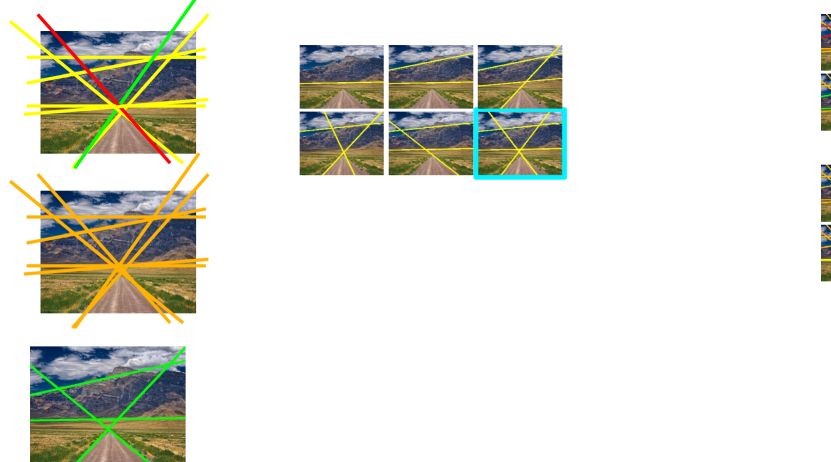
Figure 1: After selecting reliable line candidates, there are two existing approaches to semantic line detection. The first approach in (a) focuses on locating a line near a region boundary and eliminating overlapping lines. However, a redundant line still remains, since this approach does not consider how well a group of detected lines represents the layout of a scene. The second approach in (b) takes into account only the pairwise correlation between two lines, so it may fail to assess the overall harmony of more than two semantic lines. In contrast, in (c), the proposed SLCD generates a number of line combinations, analyzes all lines in each combination at once, and then finds the most harmonious combination that conveys the global scene composition optimally.

Semantic lines are essential elements in many vision applications. For example, a horizon line [32, 36, 42, 15], which is a specific type of semantic line, can be exploited to adjust the levelness of an image [16, 31]. A reflection symmetry axis [8, 4, 7, 21, 5], which is another type of semantic line, provides visual cues for object recognition and pattern analysis. Vanishing points, conveying depth impression in images, can be estimated by detecting dominant parallel semantic lines in the 3D world [41, 13, 2]. In autonomous driving systems [28, 14, 38], boundaries of road lanes can be also described by semantic lines.

Figure 2: Overview of the proposed SLCD algorithm.

Recently, several attempts [16, 13, 10, 37, 14] have been made to detect semantic lines. These techniques perform line detection and refinement sequentially. At the detection stage, they extract deep line features to classify and regress each line candidate. At the refinement stage, reliable semantic lines are determined by removing redundant lines. Specifically, to refine line candidates, non-maximum suppression (NMS) is performed in [16, 10, 13], as illustrated in Figure 1(a). Lee et al. [16] iteratively select the reliable line near boundary pixels and remove overlapping lines with the selected one. Han et al. [10] simplify the NMS process by adopting a Hough line space. Jin et al. [13] process each candidate through comparative ranking and matching. These techniques, however, do not consider the overall harmony among detected lines. To cope with this issue, Jin et al. [14] estimate the relation score for every pair of detected lines and then decide harmonious semantic lines via graph optimization. But, they may yield sub-optimal results, since only the pairwise relationships between lines are exploited, as in Figure 1(b).

In this paper, we propose a novel algorithm, called semantic line combination detector (SLCD), to find an optimal group of semantic lines. It processes all lines in a line group (or combination) simultaneously, instead of analyzing each pair of lines, to estimate the overall harmony, as in Figure 1(c). Figure 2 shows an overview of the proposed SLCD. First, we select reliable lines from line candidates and then generate a number of line combinations. Second, we score all line combinations and determine the combination with the highest score as the optimal group of semantic lines. To this end, we design two novel modules for semantic feature grouping and compositional feature extraction. We also introduce a novel loss function to guide the feature grouping module. Experimental results demonstrate that SLCD can detect semantic lines reliably on existing datasets and a new dataset, called compositionally diverse lines (CDL). Moreover, it is shown that SLCD can be used effectively in various applications.

This work has the following major contributions:

• SLCD finds an optimal combination of semantic lines by processing all lines in a line combination at once.

• We construct the CDL dataset containing compositionally diverse images with implied lines. It will be made publicly available.

• SLCD outperforms conventional detectors on most datasets. Also, its effectiveness is demonstrated in three applications: vanishing point detection, symmetry axis detection, and composition-based image retrieval.

2 Related Work

Semantic lines, located near the boundaries of different semantic regions, outline the layout and composition of an image. They play an important role in various vision applications. Horizons [32, 36, 42, 15] are a specific type of semantic lines, which can be applied to adjust the levelness of images and improve their aesthetics [16, 31]. In [41, 13, 2], dominant parallel lines in the 3D world are detected to estimate vanishing points, which convey depth impression on 2D images. Also, in [21, 8, 4, 7], reflection symmetry axes are identified to analyze the shapes of objects or patterns. These types of lines can be regarded as highly implied semantic lines. In [28, 14, 38], straight lanes are detected to aid in vehicle maneuvers in road environments. Furthermore, semantic lines are essential visual cues in photographic composition [19, 17]. They direct viewers’ attention and help to compose a visually balanced image.

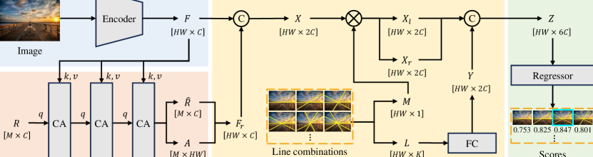
Figure 3: The architecture of SLCD. CA and FC denote cross-attention and fully connected layers, respectively. The blue, red, yellow, and green boxes indicate encoding, semantic feature grouping, compositional feature extraction, and score regression, respectively.

Several semantic line detectors [16, 10, 13, 14] have been proposed. They perform in two stages: line detection and refinement. At the detection stage, deep line features are extracted to classify and regress each line candidate. At the refinement stage, reliable semantic lines are determined by removing irrelevant candidates, based on NMS [16, 10, 13] or graph optimization [14]. More specifically, Lee et al. [16] detect reliable lines with classification probabilities higher than a threshold. They then iteratively select semantic lines and remove overlapping lines with the selected one, by employing the edge detector in [33]. Han et al. [10] predict the probability of each candidate in a Hough parametric space. They simplify NMS by computing the centroids of connected components in the Hough space. Jin et al. [13] design two comparators to estimate the priority and similarity between two lines. Then, they determine the most reliable lines and eliminate redundant ones alternately through pairwise comparisons. However, these techniques [16, 10, 13] do not consider how well a group of detected lines represents the global scene structure. To address this issue, Jin et al. [14] analyze the pairwise harmony of detected lines. They first estimate a harmony score for a pair of detected lines. They then construct a complete graph and determine harmonious semantic lines by finding a maximal weight clique. Their method, however, may yield sub-optimal results because it considers only pairwise relationships between lines. On the contrary, the proposed SLCD finds an optimal combination of semantic lines by analyzing all lines in each combination simultaneously.

3 Proposed Algorithm

We propose a novel algorithm, called SLCD, to detect an optimal combination of semantic lines, an overview of which is in Figure 2. First, we select $K$ reliable lines from line candidates and then generate a number of line combinations. Second, we score all the line combinations and determine the combination with the highest score as the optimal group of semantic lines.

3.1 Generating Line Combinations

Initializing line candidates: We generate line candidates, which are end-to-end straight lines in an image. Each line candidate is parameterized by polar coordinates in the Hough space [10]. By quantizing the coordinates uniformly, we obtain $N$ line candidates. The default $N$ is 1024.

Filtering line candidates: Given the $N$ line candidates, there are $2^{N}$ possible line combinations in total. Since this number of combinations is unmanageable, we filter out irrelevant lines to maintain $K$ reliable ones only. To this end, we design a simple line detector by modifying S-Net in [14]. Given an image, the detector obtains a convolutional feature map and extracts line features by aggregating the features of pixels along each line candidate. Then, it computes the classification probability and regression offset of each candidate. We select the most reliable candidate with the highest probability and remove overlapping lines with the selected one. We iterate this process $K$ times to determine $K$ reliable lines. The default $K$ is 8. Figure 4 shows examples of selected reliable lines. Note that, in this filtering, false negatives occur rarely because the $K$ lines are selected via NMS even though their classification probabilities are not high. The architecture of the modified S-Net is described in detail in the appendix (Section A.1).

Generating line combinations: From the $K$ reliable lines, we generate all $2^{K}$ line combinations.

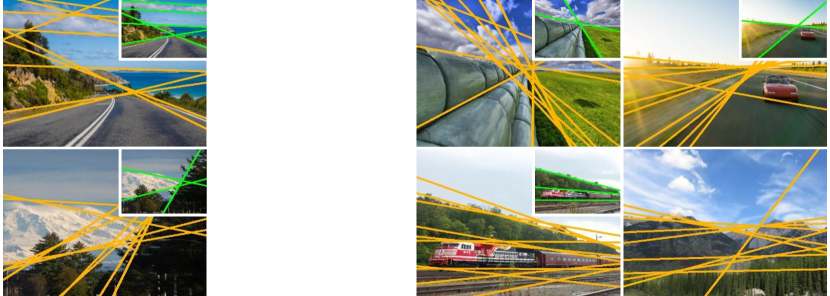
Figure 4: From a set of line candidates, the line detector selects $K$ reliable lines, depicted in orange. A high recall rate is achieved because a sufficient number of reliable lines are selected through NMS. Ground-truth semantic lines in green are in the insets.

3.2 Assessing Line Combinations

When a line combination divides an image insufficiently or over-segments it into unnecessary parts, it does not describe the overall structure of the scene properly. On the contrary, an optimal combination of semantic lines should convey the image composition reliably and efficiently (i.e. with a small number of lines). To find the best line combination, we develop the semantic line combination detector (SLCD). Figure 3 shows the structure of SLCD, which performs encoding, semantic feature grouping, compositional feature extraction, and score regression. The detailed architecture of SLCD is described in the appendix (Section A.2).

Encoding: Given an image, we extract multi-scale feature maps of ResNet50 [12]. Then, we match their spatial resolutions via bilinear interpolation and concatenate them in the channel dimension. We then squeeze the channels using 2D convolutional layers to obtain an aggregated feature map $F\in\mathbb{R}^{HW\times C}$, where $H$, $W$, and $C$ are the feature height, the feature width, and the number of channels.

Semantic feature grouping: Semantic lines are located near the boundaries between distinct regions. For their reliable detection, it is desirable to separate different regional parts more clearly. We hence attempt to group pixel features into multiple regions through cross-attention [3, 34, 35, 24]. We employ three cross-attention modules.

Let $R\in\mathbb{R}^{M\times C}$ be a learnable matrix representing $M$ regions, called region query matrix. Then, we convert $R$ into queries and $F$ into keys and values by

$$R_{q}=RU_{q},\,\,\,F_{k}=(F+S)U_{k},\,\,\,F_{v}=(F+S)U_{v},$$ (1)

where $S\in\mathbb{R}^{HW\times C}$ denotes the sinusoidal positional encoding [30], and $U_{q},U_{k},U_{v}\in\mathbb{R}^{C\times C}$ are projection matrices for queries, keys, and values. We then obtain an updated region query matrix $\hat{R}$ by

$$A=\underset{M}{\operatorname{softmax}}(R_{q}F_{k}^{\rm T}/\tau),\,\,\,\hat{R}=AF_{v}+R,$$ (2)

where $A\in\mathbb{R}^{M\times HW}$ is the attention matrix with a scaling factor $\tau$, and the letter ‘$M$’ means the softmax operation is done in the column direction, as in [34, 35, 24]. Then, in the last cross-attention, we generate a semantic feature map $F_{s}\in\mathbb{R}^{HW\times C}$ by

$$F_{s}=A^{\rm T}\hat{R}.$$ (3)

Finally, we channel-wise concatenate $F$ and $F_{s}$ to obtain a combined feature map $X\in\mathbb{R}^{HW\times 2C}$.

Note that, in (2), the softmax function is applied along the query axis. Thus, in $A=[{\mathbf{p}}_{1},{\mathbf{p}}_{2},\dots,{\mathbf{p}}_{HW}]$, each column ${\mathbf{p}}_{i}\in\mathbb{R}^{M}$ is a probability vector. Specifically, the $m$th element $p_{i}^{m}$ in ${\mathbf{p}}_{i}$ is the probability that pixel $i$ belongs to the $m$th region query. Figure 5 visualizes membership maps, computed by

$$\big{[}\operatorname{argmax}({\mathbf{p}}_{1}),\operatorname{argmax}({\mathbf{p}}_{2}),\dots,\operatorname{argmax}({\mathbf{p}}_{HW})\big{]}$$ (4)

where each element is the index of the region query that the corresponding pixel most likely belongs to. We see that each image is partitioned into $M$ meaningful regions. Thus, $F_{s}$ in (3) represents the regional membership of each pixel and is used to make the feature map $X$ more discriminative.

To produce the attention matrix $A$ reliably, we design a novel loss function in Section 3.3. The default $M$ is 8.

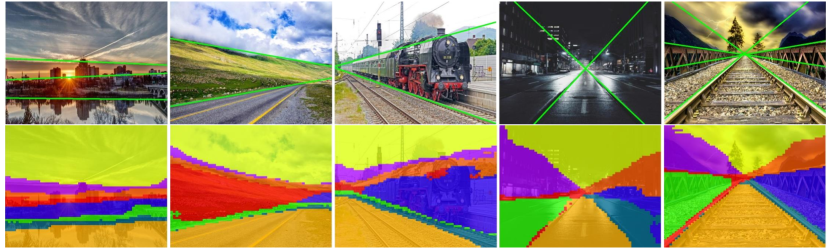
Figure 5: Visualization of semantic feature grouping results. The top row shows input images with ground-truth lines. The bottom one presents the membership maps, representing the semantic region that each pixel belongs to.

Compositional feature extraction: For each line combination, we generate three types of feature maps to extract a compositional feature map. First, we generate a binary mask $B\in\mathbb{R}^{HW}$ for each line combination. Each element in $B$ is 1 if the corresponding pixel belongs to any line in the combination, and 0 otherwise. Then, we decompose the combined feature into a line feature map $X_{l}$ and a region feature map $X_{r}$ by

$$X_{l}=X\otimes B,\,\,\,X_{r}=X\otimes(1-B),$$ (5)

where $\otimes$ is the element-wise multiplication. In other words, $X_{l}\in\mathbb{R}^{HW\times 2C}$ contains contextual information for the line pixels only, whereas $X_{r}\in\mathbb{R}^{HW\times 2C}$ does for the pixels strictly inside the regions divided by the lines.

Moreover, we generate a line collection map $L=[L_{1},L_{2},\dots,L_{K}]\in\mathbb{R}^{HW\times K}$, where $L_{k}\in\mathbb{R}^{HW}$ is a ternary mask for the $k$th reliable line, as illustrated in Figure 6. If the $k$th reliable line does not belong to the line combination, all elements in $L_{k}$ are set to 0. Otherwise, each value in $L_{k}$ is set to either $1$ or $-1$ to indicate where the corresponding pixel is located between the two parts divided by the $k$th reliable line. In other words, $L_{k}$ informs how the $k$th line splits the image into two regions. We then produce a positional feature map $P\in\mathbb{R}^{HW\times 2C}$ by applying a series of fully connected layers to $L$. Then, we yield a compositional feature map $Z\in\mathbb{R}^{HW\times 6C}$ by

$$Z=[X_{l},X_{r},P],$$ (6)

which contains information about how the lines in the combination separate the image into multiple parts.

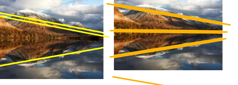
Figure 6: Illustration of the line collection map generation when $K=3$: (a) reliable lines, (b) line combinations, and (c) line collection maps.

Score regression: Lastly, using a regressor, we estimate a composition score for each line combination. Then, we declare the line combination with the highest score as the optimal group of semantic lines. The regressor takes the compositional feature map $Z$ in (6) as input and predicts a composition score $s$ within $[0,1]$. It is implemented using a bilinear interpolation layer and a series of 2D convolution layers and fully connected layers with the ReLU activation.

3.3 Loss Functions

To train SLCD, we design two loss functions.

Semantic region separation loss: When two pixels $i$ and $j$ are located in distinct regions, they should be assigned to different region queries. In other words, their probability vectors ${\mathbf{p}}_{i}$ and ${\mathbf{p}}_{j}$ in the attention matrix $A$ should be far from each other. Let $X$ and $Y$ be the two regions divided by a ground-truth line. Their probability vectors are defined as

$${\mathbf{p}}_{X}=\frac{1}{|X|}\sum_{i\in X}{\mathbf{p}}_{i},\quad\quad{\mathbf{p}}_{Y}=\frac{1}{|Y|}\sum_{j\in Y}{\mathbf{p}}_{j},$$ (7)

which should be also far from each other, for the ground-truth line divides the image into two semantic regions.

To measure the distance between probability vectors, we adopt the Kullback-Leibler divergence (KLD) [6]. Then, we define the semantic region segmentation (SRS) loss, by employing all ground-truth lines, as

$$\mathcal{L}_{\rm SRS}=-\sum_{l=1}^{T}\big{[}D({\mathbf{p}}_{X_{l}}\!\!\parallel\!{\mathbf{p}}_{Y_{l}})+D({\mathbf{p}}_{Y_{l}}\!\!\parallel\!{\mathbf{p}}_{X_{l}})\big{]}$$ (8)

where $D$ denotes the KLD, ${\mathbf{p}}_{X_{l}}$ and ${\mathbf{p}}_{Y_{l}}$ are the regions divided by the $l$th ground-truth line, and $T$ is the number of ground-truth lines. Both $D({\mathbf{p}}_{X_{l}}\!\!\parallel\!{\mathbf{p}}_{Y_{l}})$ and $D({\mathbf{p}}_{Y_{l}}\!\!\parallel\!{\mathbf{p}}_{X_{l}})$ are computed because $D$ is not commutative. With $\mathcal{L}_{\rm SRS}$, it is possible to roughly segment an image into meaningful parts, as illustrated in Figure 5, even though no ground-truth labels for semantic segmentation are used for training.

Regression loss: We also design a loss for regressing the composition score of each line combination. To this end, we employ the HIoU metric [14] that quantifies the structural layout of a line combination. Let ${\mathbf{c}}$ and ${\mathbf{c}}^{\star}$ denote a line combination and the ground-truth combination, respectively. We compute the HIoU between ${\mathbf{c}}$ and ${\mathbf{c}}^{\star}$ and use it as the ground-truth composition score ${\bar{s}}$ of ${\mathbf{c}}$. Then, the regression loss is defined as

$$\mathcal{L}_{\rm reg}=(s-{\bar{s}})^{2}$$ (9)

where $s$ is the predicted score of ${\mathbf{c}}$. To reduce $\mathcal{L}_{\rm reg}$ effectively, a ranking loss $\mathcal{L}_{\rm rank}$ is also employed as in [18].

Figure 7: The proposed CDL dataset contains 9,100 images in seven composition classes: Horizontal, Vertical, Diagonal, Triangle, Symmetric, Low, and Front. The ground-truth semantic lines are depicted in green.

4 Experimental Results

4.1 Implementation Details

We adopt ResNet50 [12] as the encoder of the proposed SLCD. We use the AdamW optimizer [20] with a learning rate $10^{-4}$, a weight decay of $10^{-4}$, $\gamma=0.5$, $\beta_{1}=0.9$, and $\beta_{2}=0.999$. We use a batch size of two for 400,000 iterations. Training images are resized to $480\times 480$ and augmented by random horizontal flipping. We fix the number of line candidates, reliable lines, and region queries to $N=1024$, $K=8$, and $M=8$, respectively. We set $H=60$, $W=60$, and $C=96$.

4.2 Datasets

SEL [16]: It is the first dataset for semantic line detection. It contains 1,750 images, which are split into 1,575 training and 175 test images. Each semantic line is annotated by the coordinates of two endpoints on an image boundary. In SEL, most images are high-quality landscapes, in which semantic lines are often obvious.

SEL_Hard [13]: It contains 300 test images only, selected from the ADE20K segmentation dataset [39]. It is challenging because of cluttered scenes or occluded objects.

NKL [37]: It is a relatively large dataset of 5,200 training and 1,300 testing images. It includes both indoor and outdoor scenes.

CDL: We construct CDL to contain 7,100 scenes with diverse contents and compositions. It is split into 6,390 training and 710 test images. As in Figure 16, the images are categorized into seven composition classes: Horizontal, Vertical, Diagonal, Triangle, Symmetric, Low, and Front. In Low and Front, humans and animals are essential parts of the image composition. In the other classes, most images are outdoor ones, as in the other datasets. To construct CDL, semantic lines were manually annotated in about 200 man-hours. More examples and the annotation process are provided in the appendix (Section B).

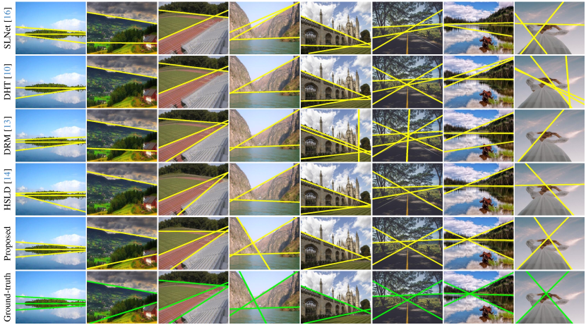
Figure 8: Comparison of detected semantic lines. From the left, two images are selected from each of the SEL, SEL_Hard, NKL, and CDL datasets.

Table 1: Comparison of the HIoU scores (%) on the SEL, SEL_Hard, NKL, and CDL datasets.

	SEL	SEL_Hard	NKL	CDL
SLNet [16]	77.87	59.71	65.49	57.78
DHT [10]	79.62	63.39	69.08	63.24
DRM [13]	80.23	68.83	67.42	63.96
HSLD [14]	81.03	65.99	74.29	64.98
Proposed	84.09	68.15	76.21	68.85

4.3 Metrics

As mentioned earlier, the harmony of detected lines is more important than individual lines in semantic line detection. Therefore, the main paper discusses only HIoU performances. The precision, recall, and f-measure results, which are metrics used in previous work, are compared in the supplemental document.

HIoU: An optimal group of semantic lines conveys a harmonious impression about the composition of an image. To assess the overall harmony of detection results, we use the HIoU metric [14]. It measures the consistency between the division of an image by detected lines and that by the ground truth. Let $S=\{s_{1},s_{2},\ldots,s_{N}\}$ and $T=\{t_{1},t_{2},\ldots,t_{M}\}$ be the regions divided by the detected lines and the ground-truth lines, respectively. Then, HIoU is computed as

$$\textstyle{\rm HIoU}=\frac{\sum_{i=1}^{N}\max_{k}{{\rm IoU}(s_{i},t_{k})}+\sum_{j=1}^{M}\max_{k}{{\rm IoU}(t_{j},s_{k})}}{N+M}.$$ (10)

Specifically, for each $s_{i}$, the most overlapping region $t_{k}$ is chosen and the intersection-over-union (IoU) is calculated. This is performed similarly for each $t_{j}$. Then, the HIoU score is given by the average of these bi-directionally matching IoUs.

4.4 Comparative Assessment

Table 1 compares the HIoU scores of the proposed SLCD with those of the existing detectors [16, 10, 13, 14] on the SEL, SEL_Hard, NKL, and CDL datasets. Also, Figure 8 compares detection results qualitatively. The existing detectors miss correct lines or fail to remove redundant lines, yielding sub-optimal results. In contrast, SLCD detects semantic lines more precisely and represents the composition more reliably than the existing detectors do. More detection results are available in the appendix (Section D).

Comparison on SEL: In Table 1, SLCD outperforms the existing detectors on SEL. Compared with the second-best HSLD, SLCD yields a wide HIoU margin of 3.06. This indicates that SLCD finds an optimal group of semantic lines more effectively by processing all lines in each combination simultaneously, instead of performing pairwise comparisons in HSLD.

Comparison on SEL_Hard: As done in [13], we conduct experiments on SEL_Hard using the networks trained on the SEL dataset. In Table 1, SLCD ranks 2nd on SEL_Hard. DRM provides a better result than SLCD, but it demands much higher complexity, as will be discussed in Section 4.5.

Table 2: Comparison of the HIoU scores (%) on the CDL dataset according to the number $M$ of region queries.

$M$	4	8	16	32
HIoU	66.43	68.85	68.11	67.07

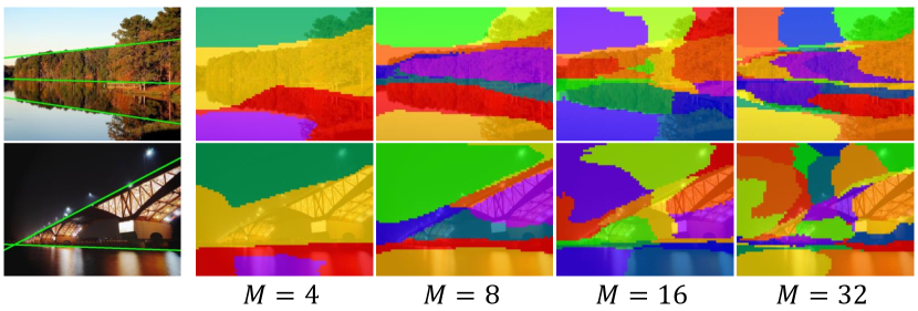
Figure 9: Visualization of the membership maps according to $M$.

Comparison on NKL: SLCD surpasses all existing detectors. For example, its HIoU score is 1.92 points higher than the second-best HSLD.

Comparison on CDL: Table 1 also lists HIoU scores on the proposed CDL dataset. For a fair comparison, we train the existing detectors on CDL using their publicly available source codes. We see that SLCD outperforms all existing detectors on CDL as well. SLNet, DHT, and DRM yield poor results because they do not consider the overall harmony of detected lines. HSLD is better than these detectors but is inferior to the proposed SLCD. We compare and discuss the detection results according to the composition classes in the appendix (Section D).

4.5 Analysis

We conduct several ablation studies to analyze each component of the proposed SLCD.

The number of $M$: Table 12(b) lists the HIoU performances on the CDL dataset, according to the number $M$ of region queries. At the default $M=8$, SLCD achieves the best performance. When $M$ is smaller or bigger than 8, the performance degrades due to under- or over-segmentation of semantic parts, respectively, as shown in Figure 9.

Efficacy of $\mathcal{L}_{\rm SRS}$: In Table 3, if the proposed SRS loss $\mathcal{L}_{\rm SRS}$ in (8) is excluded from the training, the performance drops by 2.14 points. It means that the composition analysis based on the SRS loss is essential for finding optimal line combinations.

Efficacy of compositional feature extraction: SLCD extracts the compositional feature map $Z$ for each line combination, by processing the line feature map $X_{l}$, the region feature map $X_{r}$, and the positional feature map $P$ in (6). In Table 4, Method I uses the line feature map only, while II uses the region feature map only. Method III utilizes both feature maps. Method IV, which is the proposed SLCD, uses all three maps.

Method I yields the worst result, for it uses only the contextual information near line pixels. Method II is slightly better than Method I, by exploiting the regional information. Using both line and region feature maps, III provides a better result. Moreover, IV further improves the performance significantly by utilizing the positional feature map. This is because the overall harmony is estimated more effectively, by combining the line structures in the positional feature map with scene contexts.

Table 3: Comparison of the HIoU scores (%) on the CDL dataset according to the usage of the SRS loss $\mathcal{L}_{\rm SRS}$.

	w/o $\mathcal{L}_{\rm SRS}$	Proposed
HIoU	66.71	68.85

Table 4: Ablation studies for the compositional feature extraction on the CDL dataset.

		Line	Region	Positional	HIoU
I		✓			65.12
II			✓		65.74
III		✓	✓		66.37
IV		✓	✓	✓	68.85

Runtime: Table 5 compares the runtimes of SLCD and the existing detectors in seconds per frame (spf). We use a PC with AMD Ryzen 9 3900X CPU and NVIDIA RTX 2080 GPU. The proposed SLCD takes 0.114spf, adding up 0.030spf and 0.074spf for generating and assessing line combinations, respectively. DHT is the fastest detector, but it is inferior to SLCD on all datasets. On the other hand, even though DRM performs better on SEL_Hard, it is about 8.4 times slower than SLCD.

5 Applications

We apply the proposed SLCD to three vision tasks: dominant vanishing point detection, reflection symmetry axis detection, and composition-based image retrieval. Note that the first two tasks were considered in [13]. Due to the page limit, more details and results are described in the appendix (Section E).

5.1 Dominant Vanishing Point Detection

A vanishing point (VP) facilitates understanding of the 3D geometric structure. We apply the proposed SLCD to detect dominant VPs, by identifying vanishing lines. We use the AVA landscape dataset [41], in which two dominant parallel lines are annotated for each image. To detect a dominant VP, we generate line combinations containing two lines only. We then find the best combination, whose intersecting point is declared as a VP. Table 6 compares this VP detection scheme with the existing line-based VP detectors in [41, 13]. The angle accuracies (AAs) [40] are compared. We see that SLCD is better than the existing detectors, except that its AA$1^{\circ}$ score is lower than that of Zhou et al. [41]. Figure 29 shows some VP detection results.

Table 5: Runtime comparison of the proposed SLCD and the existing detectors. The processing times are reported in seconds per frame (spf).

SLNet [16]	DHT [10]	DRM [13]	HSLD [14]	Proposed
0.136	0.033	0.952	0.046	0.114

Table 6: Comparison of the AA scores (%) of VP detection.

	AA$1^{\circ}$	AA$2^{\circ}$	AA$10^{\circ}$
Zhou et al. [41]	18.5	33.0	60.0
Jin et al. [13]	8.6	22.9	68.3
Proposed	16.6	36.9	78.3

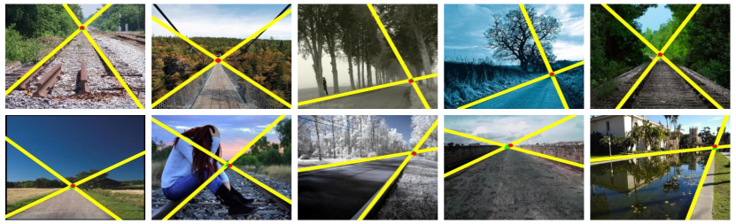
Figure 10: Detected dominant parallel lines and their intersections are depicted by yellow lines and green triangles, respectively. The ground-truth VPs are depicted by red dots.

5.2 Reflection Symmetry Axis Detection

Reflection symmetry is a visual cue for analyzing object shapes and patterns. Its detection is challenging because the symmetry is only implicit in many cases. We test the proposed SLCD on three datasets: ICCV [8], NYU [5], and SYM_Hard [13]. In these datasets, each image contains a single reflection symmetry axis. Thus, in the proposed SLCD, each of the $K$ reliable lines is regarded as a line combination. Table 7 compares the AUC_A scores [16] of the proposed SLCD and the conventional techniques [4, 7, 5, 21, 13]. SLCD outperforms all these techniques on all datasets. Figure 30 shows some detection results together with the membership maps. We see that regional parts are symmetrically divided along implied axes, enabling SLCD to identify those axes effectively.

Table 7: Comparison of the AUC_A scores (%) of symmetry axis detection.

	ICCV	NYU	SYM_Hard
Cicconet et al. [4]	80.80	82.85	68.99
Elawady et al. [7]	87.24	83.83	73.90
Cicconet et al. [5]	87.38	87.64	81.04
Loy & Eklundh [21]	89.77	90.85	81.99
Jin et al. [13]	90.60	92.78	84.73
Proposed	93.15	93.51	88.03

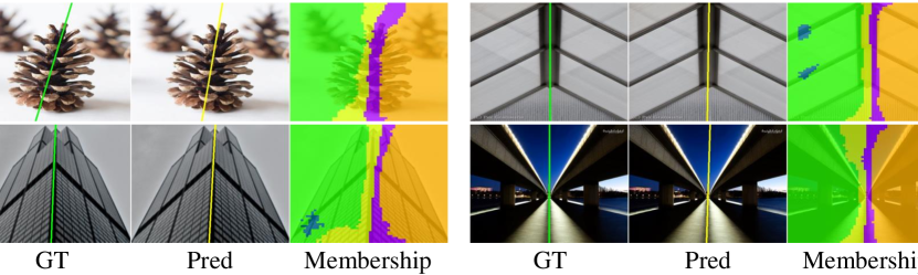
Figure 11: Symmetry axis detection results. In the top row, the ground-truth and predicted axes are depicted by dashed red and solid yellow lines, respectively. The membership maps are also visualized in the bottom row.

5.3 Composition-Based Image Retrieval

Existing image retrieval techniques focus on the visual contents of a query image to find similar images in a database [22, 26, 9, 27]. In this work, however, we attempt to discover images with similar compositions to a query image, i.e. composition-based image retrieval.

We test the proposed SLCD on the Oxford 5k and Paris 6k retrieval dataset [25]. We first detect semantic lines in every image, while storing the positional feature map $P$ in (6). We filter out some images whose composition scores are lower than a threshold since a low score indicates a low-quality image with inharmonious composition in general. Then, for a randomly selected query image, we compute the $\ell_{2}$-distances between the positional feature maps $P$ of the query and the remaining images. We determine the images with the smallest distances as retrieval results.

Figure 31 shows the top-4 retrieval results for four query images. We see that SLCD returns structurally similar images to the queries. This means that the positional feature maps $P$, containing the structural information of semantic lines, can be used to compute the compositional differences. Based on this observation, we perform data clustering by employing k-means [11] on the feature space of $P$. Figure 13 is t-SNE visualization [29] of the clustering results. The nine images nearest to each centroid are also shown. Note that images with similar composition are grouped into the same cluster, confirming the efficacy of SLCD in the compositional analysis of images.

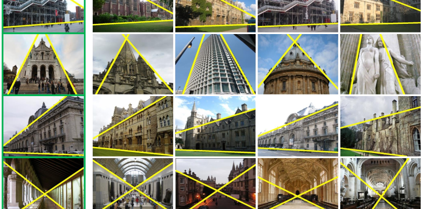
Figure 12: Composition-based retrieval results for query images.

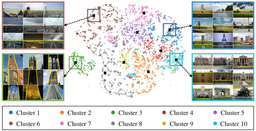
Figure 13: t-SNE visualization [29] of the feature space for the Oxford 5k and Paris 6k dataset [25].

6 Conclusions

We proposed a novel semantic line detector, SLCD, which processes a combination of lines at once to estimate the overall harmony reliably. We first generated all possible line combinations from reliable lines. Then, we estimated the score of each line combination and determined the best combination. Experimental results demonstrated that the proposed SLCD can detect semantic lines reliably on existing datasets, as well as on the new dataset CDL. Furthermore, SLCD can be successfully used in vanishing point detection, symmetry axis detection, and image retrieval.

Appendix A Implementation Details

A.1 Line detector

We design a line detector by modifying S-Net in [14] to select $K$ reliable lines from a set of line candidates. Figure 14 shows the structure of the modified line detector performing three steps: encoding, classification/regression, and NMS.

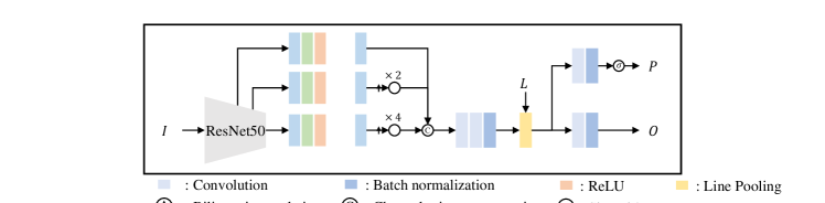
Figure 14: The architecture of the modified line detector.

Encoding: Given an image, the encoder extracts a convolutional feature map $X\in\mathbb{R}^{H\times W\times C}$. Specifically, we first extract multi-scale feature maps (the three coarsest feature maps) using ResNet50 [12] as the backbone. We then match each channel dimension to $C$ by applying a pair of $3\times 3$ dilated convolutional layers with batch normalization and ReLU activation. We also match the resolutions of the two coarser maps to the finest one using bilinear interpolation and concatenate them. Finally, We obtain a combined feature map $X$ by applying two $3\times 3$ dilated convolutional layers and one $3\times 3$ convolutional layer.

Classification and regression: A line candidate, which is an end-to-end straight line in an image, can be parameterized by polar coordinates in the Hough space [10]. Let $l=(\rho,\theta)$ denote a line, where $\rho$ is the distance from the center of the image and $\theta$ is its angle from the $x$-axis. Then, we generate an initial set of $N$ line candidates, $L=[l_{1},l_{2},\dots,l_{N}]\in\mathbb{R}^{N\times 2}$, by quantizing $\rho$ and $\theta$ uniformly. For the $N$ line candidates, we predict a probability vector $P\in\mathbb{R}^{N\times 1}$ and an offset matrix $O\in\mathbb{R}^{N\times 2}$. To this end, we extract a line feature matrix $X_{l}\in\mathbb{R}^{N\times C}$ of $L$ by employing a line pooling layer [16]. Then, we feed $X_{l}$ into classification and regression layers to predict $P$ and $O$, respectively. More specifically, $P=\sigma(f_{1}(G))$ and $O=f_{2}(G)$, where $f_{1}$ and $f_{2}$ consist of two fully-connected layers, respectively, and $\sigma(\cdot)$ is the sigmoid function. Then, we update the line candidates by $\hat{L}=L+O$.

NMS: We select $K$ reliable lines from the updated set $\hat{L}$ based on the line probability matrix $P$. Specifically, we select the line with the highest probability and then remove the overlapping lines, whose $L_{2}$-distances in polar coordinates from the selected one are lower than a threshold. We iterate this process $K$ times to determine $K$ reliable lines.

Generating line combinations: From the $K$ reliable lines, we generate all $2^{K}$ line combinations. This process is done in parallel. Specifically, we compose a combination matrix ${\mathbf{C}}=[{\mathbf{c}}_{1},{\mathbf{c}}_{2},\dots,{\mathbf{c}}_{2^{K}}]\in\mathbb{R}^{K\times 2^{K}}$. Each column ${\mathbf{c}}_{i}\in\mathbb{R}^{K}$ is a boolean vector, where the $k$th element ${\mathbf{c}}_{i}^{k}$ is set to 1 if the $k$th reliable line belongs to the $i$th line combination, and 0 otherwise.

A.2 SLCD

We develop the semantic line combination detector (SLCD) to find the best line combination. The structure of SLCD is shown in Figure 3 in the main paper. It performs four steps: encoding, semantic feature grouping, compositional feature extraction, and score regression. Here, we describe the semantic feature grouping and score regression steps in detail.

Semantic feature grouping: Figure 15 (a) and (b) show the semantic feature grouping module and its cross-attention (CA) block, respectively. In Figure 15 (a), the module updates the region query matrix $R$ three times using CA blocks. Each CA block takes $F$ and $R$ as input and yields updated region query matrix $\hat{R}$. In the last block, it additionally outputs the attention matrix $A$. In Figure 15 (b), LN and MLP denote layer normalization and multi-layer perceptron, respectively. The MLP consists of two fully connected layers with ReLU activation. Also, the projection matrices $U_{q},U_{k},U_{v}\in\mathbb{R}^{C\times C}$ are implemented by a fully connected layer.

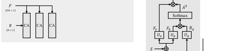
Figure 15: The architectures of the semantic feature grouping module and its cross-attention block.

Score regression: We assess each line combination using a regressor. The regressor takes the compositional feature map $Z\in\mathbb{R}^{HW\times 6C}$ as input and predicts a composition score $s$. More specifically, we first obtain a reduced feature map by $Z^{\prime}=f(\psi(Z))\in\mathbb{R}^{\frac{H}{4}\frac{W}{4}\times C}$, where $\psi$ is the bilinear interpolation to reduce the resolution by a factor of $\frac{1}{4}$. Also, $f$ consists of 2D convolution layers to reduce the channel dimension to $C$. We then estimate the score by $s=g(\bar{Z^{\prime}})$, where $\bar{Z^{\prime}}$ is a flattened $Z^{\prime}$, and $g$ consists of a series of fully connected layers with ReLU activation.

A.3 Training and hyper-parameters

Let us describe the training process of the modified line detector in detail.

Line detector: We generate a ground-truth (GT) line probability vector $\bar{P}\in\mathbb{R}^{N\times 1}$ and a GT offset matrix $\bar{O}\in\mathbb{R}^{N\times 2}$. Specifically, we set $\bar{P}_{l}=1$ if the $L_{2}$-distance in polar coordinates between a line candidate and the best matching GT line is lower than a threshold, and $\bar{P}_{l}=0$ otherwise. Also, we obtain $\bar{O}_{l}$ by computing the offset vector between a line candidate $l$ and its matching GT line. To train the modified line detector, we minimize the loss

$$\mathcal{L}=\lambda_{1}\ell_{\rm cls}(P,\bar{P})+\lambda_{2}\ell_{\rm reg}(O,\bar{O})$$ (11)

where $\ell_{\rm cls}$ is the cross-entropy loss, and $\ell_{\rm reg}$ is the smooth $L_{1}$ loss. We set $\lambda_{1}$ and $\lambda_{2}$ to 1 and 5, respectively. We use the AdamW optimizer [20] with an initial learning rate of $10^{-4}$ and halve it after every 80,000 iterations five times. We use a batch size of eight. Also, we resize training images to $480\times 480$ and augment them via random horizontal flipping and random rotation between $-5^{\circ}$ and $5^{\circ}$.

Hyper-parameters: Table 8 lists the hyper-parameters in the proposed algorithm. We will make the source codes publicly available.

Table 8: Hyper-parameter settings.

Line detector	Description	SLCD	Description
$H=60$	Feature height	$H=60$	Feature height
$W=60$	Feature width	$W=60$	Feature width
$C=96$	# of feature channels	$C=96$	# of feature channels
$N=1024$	# of line candidates	$M=8$	# of region queries
$K=8$	# of reliable lines	$\tau=1$	scaling factor

Appendix B CDL Dataset

B.1 Data preparation

Semantic lines represent the layout and composition of an image. Despite the close relationship between semantic lines and photographic composition, existing semantic line datasets do not consider image composition. To assess semantic line detection results for various types of composition, we construct a compositionally diverse semantic line dataset, called CDL, in which the photos are categorized into seven composition classes: Horizontal, Vertical, Diagonal, Triangle, Symmetric, Low, and Front. In Low and Front, humans and animals are essential parts of the image composition. In the other classes, most images are outdoor ones, as in the other datasets. CDL contains 7,100 scenes split into 6,390 training and 710 test images. Figure 16 shows example images and annotations in the proposed CDL.

Figure 16: Example images and annotations in the proposed CDL dataset.

B.2 Manual annotation

For each image, we annotated the start and end points of each semantic line. We employed an annotation tool, CVAT [1], as shown in Figure 17. We adjusted the coordinates of each line so that the lines represented the image composition optimally and harmoniously. Eight people inspected each annotated image, and unsatisfactory annotations were identified and re-annotated. The inspection was repeated until a consensus was made. The manual annotation process took more than 200 man-hours.

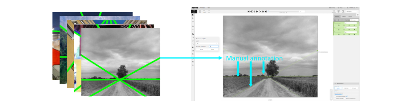
Figure 17: Manual annotation process of semantic lines using CVAT. Ground-truth lines are depicted in green.

Appendix C More analysis

C.1 Performances

Table 9 reports the performances on the SEL and SEL_Hard datasets. We compare the area under curve (AUC) performances of the precision, recall, and F-measure curves, which are denoted by AUC_P, AUC_R, and AUC_F, respectively [16]. Also, Table 10 compares the EA-scores [37] on the NKL and proposed CDL datasets. Note that, unlike HIoU [14], AUC performances and EA-scores do not consider the overall harmony of detected lines. They only consider the positional accuracy of each detected line. We see that the proposed SLCD provides better results on most datasets in terms of detecting harmonious lines while accurately identifying individual lines.

Table 9: Comparison of the AUC and HIoU on the SEL and SEL_Hard datasets.

	SEL					SEL_Hard
	AUC_P	AUC_R	AUC_F	HIoU		AUC_P	AUC_R	AUC_F	HIoU
SLNet [16]	80.72	84.22	82.43	77.87		74.22	70.68	72.41	59.71
DHT [10]	87.74	80.25	83.83	79.62		83.55	67.98	75.09	63.39
DRM [13]	85.44	86.87	86.15	80.23		87.19	77.69	82.17	68.83
HSLD [14]	89.61	83.93	86.68	81.03		87.60	72.56	79.38	65.99
Proposed	95.27	80.03	86.99	84.09		90.32	70.14	78.96	68.15

Table 10: Comparison of the EA-scores and HIoU on the NKL and CDL datasets.

	NKL					CDL
	Precision	Recall	F-measure	HIoU		Precision	Recall	F-measure	HIoU
SLNet [16]	74.41	74.50	74.45	65.49		63.99	74.08	68.61	57.78
DHT [10]	78.76	83.17	80.88	69.08		72.02	79.49	75.52	63.24
DRM [13]	74.27	79.28	76.67	67.42		72.80	72.13	72.46	63.96
HSLD [14]	79.60	81.14	80.36	74.29		71.74	75.86	73.73	64.98
Proposed	84.39	80.60	82.44	76.21		75.69	78.41	77.02	68.85

Table 11 shows the HIoU scores on the proposed CDL dataset according to the composition classes. We train the existing detectors on CDL using their publicly available source codes. We see that the proposed SLCD outperforms all the existing techniques in all classes without exception. Among the seven classes, Low and Front are challenging ones because the complex boundaries of objects (humans or animals) make it difficult to identify the implied semantic lines. Qualitative results are shown in Section D.3.

Table 11: Comparison of the HIoU scores (%) according to the composition classes in the CDL dataset.

	Horizontal	Vertical	Diagonal	Triangle	Symmetric	Low	Front	Total
SLNet [16]	72.67	51.32	64.52	47.04	69.18	46.87	49.25	57.78
DHT [10]	76.02	59.70	64.87	59.45	65.61	47.82	60.43	63.24
DRM [13]	75.86	61.19	67.86	51.69	69.09	49.68	63.41	63.96
HSLD [14]	76.43	60.36	69.01	58.35	69.66	54.91	60.75	64.98
Proposed	77.55	66.15	72.87	67.89	72.03	57.13	64.84	68.85

C.2 Ablations

$N$ and $K$: As described in Section 3.1 in the main paper, to generate a manageable number of line combinations, we filter out redundant line candidates and obtain $K$ reliable lines. Table 12(b) lists the performances according to the number $N$ of line candidates and the number $K$ of reliable lines on CDL: (a) Recall (EA-score) rate of the line detector according to $N$, and (b) HIoU of the proposed SLCD according to $K$. The processing times are also reported in seconds per frame (spf).

In Table 12(b) (a), as $N$ increases, the recall rate gets higher. However, too large values of $N$ make the training of the line detector challenging, yielding a lower recall rate at $N=1444$, compared to $N=1024$. Hence, we set $N=1024$. In Table 12(b) (b), as $K$ increases, the HIoU score gets higher. At $K=10$, SLCD achieves the highest HIoU, but it becomes too slow. It takes 4 times longer at $K=10$ than at $K=8$, whereas their HIoU gap is 0.27 only. As a tradeoff between performance and speed, we set $K=8$.

Table 12: Comparison of the performance according to the number $N$ of line candidates and the number $K$ of reliable lines on CDL.

$K=8$	Line detector
$N\vartriangleright$	400	900	1024	1444
Recall	88.61	90.16	91.77	91.23
spf	0.027	0.028	0.030	0.032

(a) Recall rate of the line detector according to $N$

$N=1024$	SLCD
$K\vartriangleright$	6	8	10
HIoU	67.96	68.85	69.12
spf	0.033	0.074	0.316

(b) HIoU of SLCD according to $K$.

C.3 Visualizations

Sorting results according to composition scores: Note that we determine an optimal group of semantic lines in an image, by finding the line combination with the highest composition score, estimated by the proposed SLCD. Figure 18 (b) and (c) show examples of top-4 and bottom-4 line combinations, respectively. The top-4 detection results represent image composition faithfully. In contrast, the bottom-4 detection results represent it poorly. These examples indicate that the proposed SLCD evaluates each line combination reliably based on composition analysis.

Figure 18: Sorting of line combinations based on predicted composition scores: (a) ground-truth lines, (b) top-4 line combinations, and (c) bottom-4 line combinations.

Appendix D Qualitative Results

D.1 Comparison on SEL and SEL_Hard

Figure 19 and Figure 20 compare the proposed SLCD with conventional algorithms on SEL and SEL_Hard, respectively. SLCD provides better detection results than the conventional algorithms.

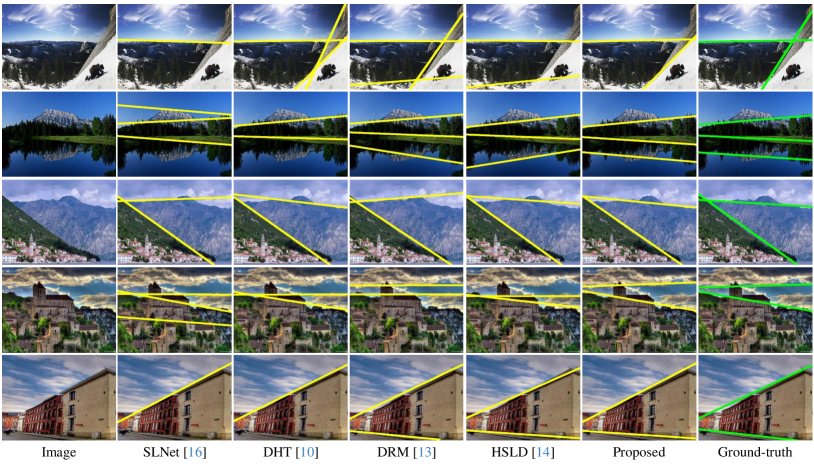
Figure 19: Comparison of semantic line detection results on the SEL dataset.

Figure 20: Comparison of semantic line detection results on the SEL_Hard dataset.

D.2 Comparison on NKL

Figure 21 compares the proposed SLCD with existing line detectors on NKL.

Figure 21: Comparison of semantic line detection results on the NKL dataset.

D.3 Comparison on CDL

Figures 22$\sim$28 compare semantic line detection results of the proposed CDL with those of the conventional algorithms on the Horizontal, Vertical, Diagonal, Triangle, Symmetric, Low, and Front classes in the CDL dataset, respectively. We see that the proposed algorithm provides more reliable detection results consistently.

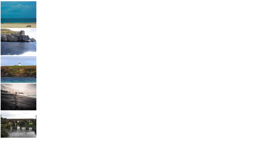
Figure 22: Comparison of semantic line detection results on the Horizontal class in the CDL dataset.

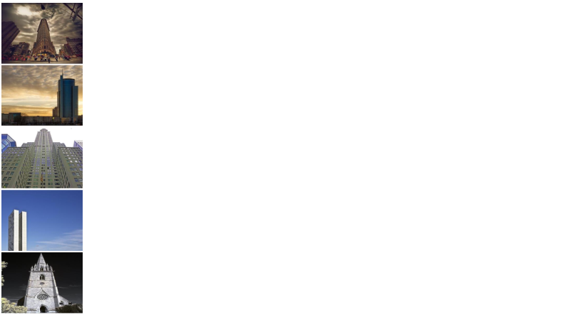
Figure 23: Comparison of semantic line detection results on the Vertical class in the CDL dataset.

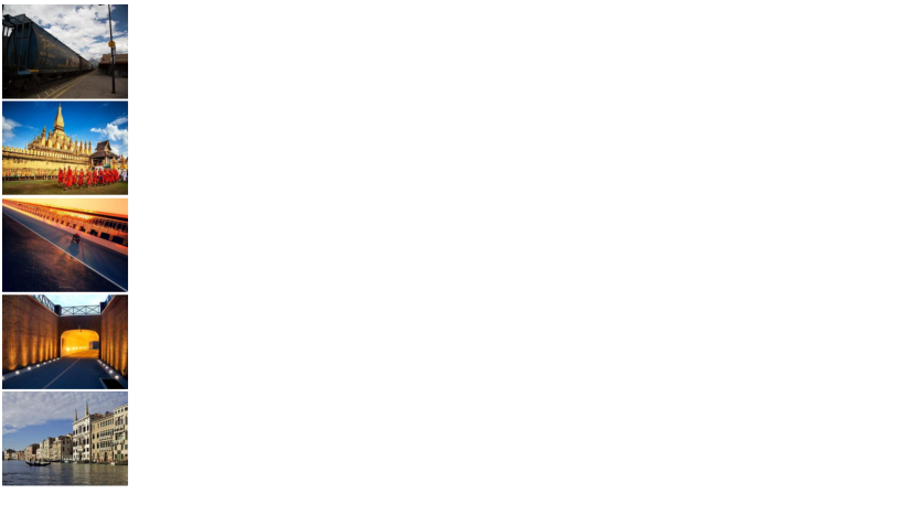
Figure 24: Comparison of semantic line detection results on the Diagonal class in the CDL dataset.

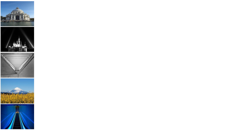
Figure 25: Comparison of semantic line detection results on the Triangle class in the CDL dataset.

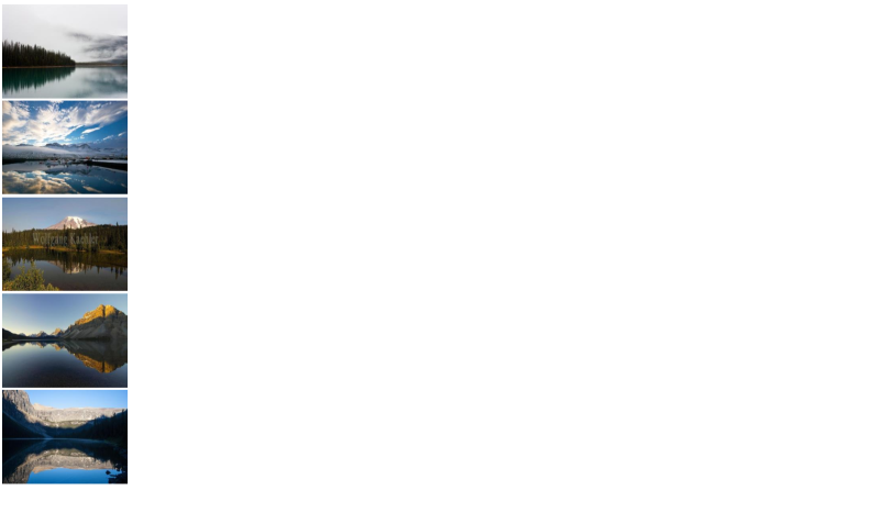
Figure 26: Comparison of semantic line detection results on the Symmetric class in the CDL dataset.

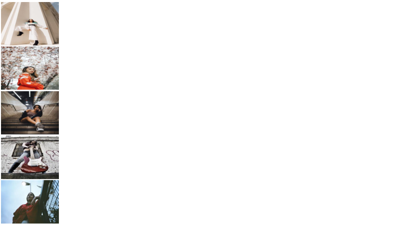
Figure 27: Comparison of semantic line detection results on the Low class in the CDL dataset.

Figure 28: Comparison of semantic line detection results on the Front class in the CDL dataset.

Appendix E Applications

E.1 Dominant vanishing point detection

We apply the proposed SLCD to detect dominant vanishing points by identifying the vanishing lines. We declare the intersecting point of two lines as a vanishing point. We assess the proposed SLCD on the AVA landscape dataset [41] which contains 2,000 training and 275 test landscape images. Figure 29 shows more results of vanishing point detection.

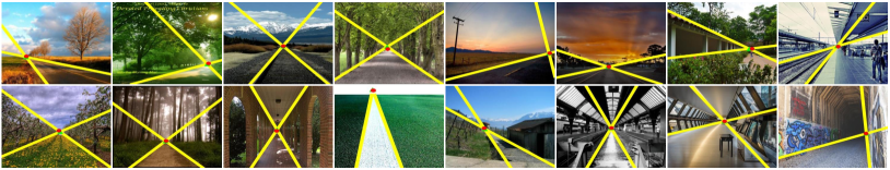
Figure 29: More results of vanishing point detection.

E.2 Reflection symmetry axis detection

We test the proposed SLCD on three datasets: ICCV [8], NYU [5], and SYM_Hard [13]. ICCV provides 100 training and 96 test images, NYU contains 176 test images, and SYM_Hard consists of 45 test images. In these datasets, each images contains a single reflection symmetry axis. We trained the model on the ICCV and tested it on all datsets. Figure 30 shows more results of vanishing point detection. In the top row, the ground-truth and predicted axes are depicted by dashed red and solid yellow lines, respectively. The membership maps are also visualized in the bottom row.

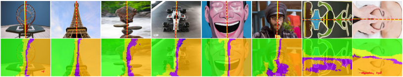
Figure 30: More results of symmetric axis detection.

E.3 Composition-based image retrieval

We test the proposed SLCD on Oxford 5k and Paris 6k dataset [25], containing photographs of landmarks and local attractions in two places. Since it contains indoor and outdoor images mainly, we use the network trained on NKL dataset. We first detect semantic lines for all the images, while storing the positional feature map $P$. Then, we filter out images whose the composition scores are lower than a threshold $0.75$ since a low score indicates a low quality image with inharmonious composition, as shown in Figure 18. Then, for a randomly selected query image, we compute the $\ell_{2}$-distances between the positional feature maps $P$ of the query and the remaining images. We determine the images with the smallest distances as retrieval results. Figure 31 shows more results of composition-based retrieval.

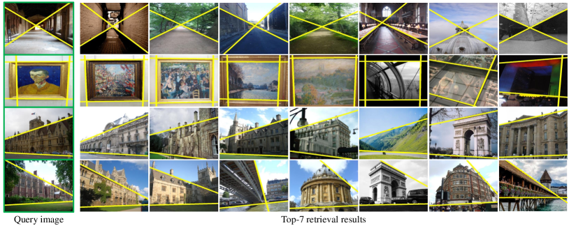
Figure 31: More results of composition-based retrieval.

E.4 Road lane detection

We apply the proposed SLCD to the lane detection task, by employing the CULane dataset [23]. CULane is a road lane dataset in which lanes are annotated with 2D coordinates. To obtain ground-truth semantic lines corresponding to the lanes in an image, we declare the most overlapping line with each lane as a semantic line. Figure 32 shows some examples of original lane points and ground-truth semantic lines, depicted by red dots and green lines, respectively.

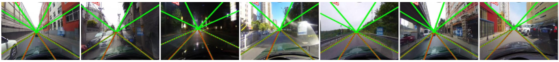
Figure 32: Examples of original lane points and ground-truth semantic lines.

We train SLCD and compare it with the second-best line detector HSLD [14]. Figure 33 shows some lane detection results on the test set. SLCD detects semantic lines more reliably in road scenes than HSLD does, even though some lines are implied due to occlusion or poor illumination. Table 13 compares the HIoU and AUC results. We see that SLCD outperforms HSLD meaningfully.

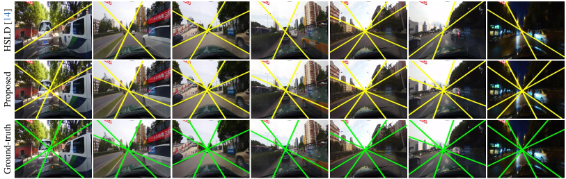
Figure 33: Comparison of semantic line detection results on the CULane dataset.

Table 13: Comparison of the HIoU and AUC results on the CULane dataset.

	AUC_P	AUC_R	AUC_F	HIoU
HSLD [14]	92.38	80.11	85.80	74.14
Proposed	92.91	84.86	88.55	76.97

References

- [1] CVAT. [Online]. Available: https://www.cvat.ai/.
- Bazin et al. [2012] Jean-Charles Bazin, Yongduek Seo, Cédric Demonceaux, Pascal Vasseur, Katsushi Ikeuchi, Inso Kweon, and Marc Pollefeys. Globally optimal line clustering and vanishing point estimation in manhattan world. In Proc. IEEE CVPR, 2012.
- Carion et al. [2020] Nicolas Carion, Francisco Massa, Gabriel Synnaeve, Nicolas Usunier, Alexander Kirillov, and Sergey Zagoruyko. End-to-end object detection with transformers. In Proc. ECCV, 2020.
- Cicconet et al. [2017a] Marcelo Cicconet, Vighnesh Birodkar, Mads Lund, Michael Werman, and Davi Geiger. A convolutional approach to reflection symmetry. Pattern Recog. Lett., 95:44–50, 2017a.
- Cicconet et al. [2017b] Marcelo Cicconet, David GC Hildebrand, and Hunter Elliott. Finding mirror symmetry via registration and optimal symmetric pairwise assignment of curves: Algorithm and results. In Proc. IEEE ICCV Workshops, 2017b.
- Cover and Thomas [2006] Thomas M. Cover and Joy A. Thomas. Elements of Information Theory. Wiley, 2nd edition, 2006.
- Elawady et al. [2017] Mohamed Elawady, Christophe Ducottet, Olivier Alata, Cécile Barat, and Philippe Colantoni. Wavelet-based reflection symmetry detection via textural and color histograms. In Proc. IEEE ICCV Workshops, 2017.
- Funk et al. [2017] Christopher Funk, Seungkyu Lee, Martin R Oswald, Stavros Tsogkas, Wei Shen, Andrea Cohen, Sven Dickinson, and Yanxi Liu. 2017 ICCV Challenge: Detecting symmetry in the wild. In Proc. IEEE ICCV, 2017.
- Gordo et al. [2017] Albert Gordo, Jon Almazan, Jerome Revaud, and Diane Larlus. End-to-end learning of deep visual representations for image retrieval. Int. J. Comput. Vis., 124:237–254, 2017.
- Han et al. [2020] Qi Han, Kai Zhao, Jun Xu, and Ming-Ming Cheng. Deep hough transform for semantic line detection. In Proc. ECCV, 2020.
- Hartigan and Wong [1979] J. A. Hartigan and M. A. Wong. A K-means clustering algorithm. Journal of the Royal Statistical Society. Series C (Applied Statistics), 28(1):100–108, 1979.
- He et al. [2016] Kaiming He, Xiangyu Zhang, Shaoqing Ren, and Jian Sun. Deep residual learning for image recognition. In Proc. IEEE CVPR, 2016.
- Jin et al. [2020] Dongkwon Jin, Jun-Tae Lee, and Chang-Su Kim. Semantic line detection using mirror attention and comparative ranking and matching. In Proc. ECCV, 2020.
- Jin et al. [2021] Dongkwon Jin, Wonhui Park, Seong-Gyun Jeong, and Chang-Su Kim. Harmonious semantic line detection via maximal weight clique selection. In Proc. IEEE CVPR, 2021.
- Kluger et al. [2020] Florian Kluger, Hanno Ackermann, Michael Ying Yang, and Bodo Rosenhahn. Temporally consistent horizon lines. In Proc. IEEE ICRA, 2020.
- Lee et al. [2017] Jun-Tae Lee, Han-Ul Kim, Chul Lee, and Chang-Su Kim. Semantic line detection and its applications. In Proc. IEEE ICCV, 2017.
- Lee et al. [2018] Jun-Tae Lee, Han-Ul Kim, Chul Lee, and Chang-Su Kim. Photographic composition classification and dominant geometric element detection for outdoor scenes. J. Vis. Commun. Image Represent., 55:91–105, 2018.
- Li et al. [2020] Debang Li, Junge Zhang, Kaiqi Huang, and Ming-Hsuan Yang. Composing good shots by exploiting mutual relations. In Proc. IEEE CVPR, 2020.
- Liu et al. [2010] Ligang Liu, Renjie Chen, Lior Wolf, and Daniel Cohen-Or. Optimizing photo composition. Computer Graphics Forum, 29:469–478, 2010.
- Loshchilov and Hutter [2017] Ilya Loshchilov and Frank Hutter. Decoupled weight decay regularization. arXiv preprint arXiv:1711.05101, 2017.
- Loy and Eklundh [2006] Gareth Loy and Jan-Olof Eklundh. Detecting symmetry and symmetric constellations of features. In Proc. ECCV, 2006.
- Noh et al. [2017] Hyeonwoo Noh, Andre Araujo, Jack Sim, Tobias Weyand, and Bohyung Han. Large-scale image retrieval with attentive deep local features. In Proc. IEEE ICCV, 2017.
- Pan et al. [2018] Xingang Pan, Jianping Shi, Ping Luo, Xiaogang Wang, and Xiaoou Tang. Spatial as deep: Spatial cnn for traffic scene understanding. In AAAI, 2018.
- Piccinelli et al. [2023] Luigi Piccinelli, Christos Sakaridis, and Fisher Yu. iDisc: Internal discretization for monocular depth estimation. In Proc. IEEE CVPR, 2023.
- Radenović et al. [2018a] Filip Radenović, Ahmet Iscen, Giorgos Tolias, Yannis Avrithis, and Ondřej Chum. Revisiting Oxford and Paris: Large-scale image retrieval benchmarking. In Proc. IEEE CVPR, 2018a.
- Radenović et al. [2018b] Filip Radenović, Giorgos Tolias, and Ondřej Chum. Fine-tuning CNN image retrieval with no human annotation. IEEE Trans. Pattern Anal. Mach. Intell., 41:1655–1668, 2018b.
- Smeulders et al. [2000] Arnold WM Smeulders, Marcel Worring, Simone Santini, Amarnath Gupta, and Ramesh Jain. Content-based image retrieval at the end of the early years. IEEE Trans. Pattern Anal. Mach. Intell., 22:1349–1380, 2000.
- Tabelini et al. [2021] Lucas Tabelini, Rodrigo Berriel, Thiago M. Paixao, Claudine Badue, Alberto F. De Souza, and Thiago Oliveira-Santos. Keep your eyes on the lane: Real-time attention-guided lane detection. In Proc. IEEE CVPR, 2021.
- Van der Maaten and Hinton [2008] Laurens Van der Maaten and Geoffrey Hinton. Visualizing data using t-SNE. Journal of Machine Learning Research, 9(11), 2008.
- Vaswani et al. [2017] Ashish Vaswani, Noam Shazeer, Niki Parmar, Jakob Uszkoreit, Llion Jones, Aidan N Gomez, Łukasz Kaiser, and Illia Polosukhin. Attention is all you need. In Proc. NeurIPS, 2017.
- Wang et al. [2023] Yaoting Wang, Yongzhen Ke, Kai Wang, Jing Guo, and Shuai Yang. Spatial-invariant convolutional neural network for photographic composition prediction and automatic correction. J. Vis. Commun. Image Represent., 90:103751, 2023.
- Workman et al. [2016] Scott Workman, Menghua Zhai, and Nathan Jacobs. Horizon lines in the wild. In Proc. BMVC, 2016.
- Xie and Tu [2015] Saining Xie and Zhuowen Tu. Holistically-nested edge detection. In Proc. IEEE ICCV, 2015.
- Yu et al. [2022a] Qihang Yu, Huiyu Wang, Dahun Kim, Siyuan Qiao, Maxwell Collins, Yukun Zhu, Hartwig Adam, Alan Yuille, and Liang-Chieh Chen. CMT-DeepLab: Clustering mask transformers for panoptic segmentation. In Proc. IEEE CVPR, 2022a.
- Yu et al. [2022b] Qihang Yu, Huiyu Wang, Siyuan Qiao, Maxwell Collins, Yukun Zhu, Hartwig Adam, Alan Yuille, and Liang-Chieh Chen. k-means mask transformer. In Proc. ECCV, 2022b.
- Zhai et al. [2016] Menghua Zhai, Scott Workman, and Nathan Jacobs. Detecting vanishing points using global image context in a non-manhattan world. In Proc. IEEE CVPR, 2016.
- Zhao et al. [2021] Kai Zhao, Qi Han, Chang-Bin Zhang, Jun Xu, and Ming-Ming Cheng. Deep hough transform for semantic line detection. IEEE Trans. Pattern Anal. Mach. Intell., 44:4793–4806, 2021.
- Zheng et al. [2022] Tu Zheng, Yifei Huang, Yang Liu, Wenjian Tang, Zheng Yang, Deng Cai, and Xiaofei He. CLRNet: Cross layer refinement network for lane detection. In Proc. IEEE CVPR, 2022.
- Zhou et al. [2017a] Bolei Zhou, Hang Zhao, Xavier Puig, Sanja Fidler, Adela Barriuso, and Antonio Torralba. Scene parsing through ADE20K dataset. In Proc. IEEE CVPR, 2017a.
- Zhou et al. [2019] Yichao Zhou, Haozhi Qi, Jingwei Huang, and Yi Ma. NeurVPS: Neural vanishing point scanning via conic convolution. In Proc. NeurIPS, 2019.
- Zhou et al. [2017b] Zihan Zhou, Farshid Farhat, and James Z Wang. Detecting dominant vanishing points in natural scenes with application to composition-sensitive image retrieval. IEEE Trans. Multimedia, 19:2651–2665, 2017b.
- Zhu et al. [2020] Rui Zhu, Xingyi Yang, Yannick Hold-Geoffroy, Federico Perazzi, Jonathan Eisenmann, Kalyan Sunkavalli, and Manmohan Chandraker. Single view metrology in the wild. In Proc. ECCV, 2020.