Quantum entanglement in a pure state of strongly correlated quantum impurity systems

Abstract

We consider quantum entanglement in strongly correlated quantum impurity systems for states manifesting interesting properties such as multi-level Kondo effect and dual nature between itineracy and localization etc.. For this purpose, we set up a system consisting of one or two quantum impurities arbitrarily selected from the system as a subsystem, and investigate quantum entanglement with its environmental system. We reduce the pure state of interest as described above to the subsystem, and formulate quantum informative quantities such as entanglement entropy, mutual information and relative entropy. We apply them to the single impurity Anderson model where the most basic Kondo effect is manifested, and obtain new insights into the Kondo effect there. The obtained results suggest that the method proposed here is promising for elucidating the quantum entanglement of pure states in various quantum impurity systems.

I Introduction

In solid-state electron systems, interesting ground states emerge at low temperatures as a result of the interaction of many electrons. Understanding the ground state itself is one of the central issues, which is especially difficult in strongly correlated electron systems where correlation effects between electrons cannot be ignored. In addition, the question of the quantum entanglement transitions from high temperature to low temperature to reach the ground state is interesting and important from the viewpoint of understanding the ground state from a new perspective. In recent years, quantum entanglement for interesting phenomena in crystalline systems has been studiedent , including area laws and their deviations etc..

In this paper, we primarily focus on strongly correlated quantum impurity systems and discuss quantum entanglement in such systemsCosti and H. (2003); He and Millis (2017, 2019); Kohn and Santoro (2022). A system in which multiple quantum dots are connected to electron reservoirs such as conduction electron systems is a typical strongly correlated quantum impurity system. In such a system, electron correlation effects such as the Kondo effect can be studied under controlled conditionsDehollain et al. (2020); Goldhaber-Gordon et al. (1998a, b); Potok et al. (2007); Cronenwett et al. (1998); Jeong et al. (2001); Iftikhar et al. (2015); Sasaki et al. (2000); Kobayashi et al. (2010).

It has been theoretically pointed out that various interesting ground state such as Nagaoka ferromagnetism and Lieb ferrimagnetism can be realized on multiple quantum dotsLieb and Mattis (1962); Lieb (1989); Nagaoka.Y (1965, 1966); Tasaki (2020); Buterakos and Das Sarma (2019); Tokuda and Nishikawa (2022), and experimentally, Nagaoka ferromagnetism has been realized on quartet quantum dotsDehollain et al. (2020). These states are generally entangled states among multiple quantum dotsTokuda and Nishikawa (2022); Numata et al. (2009). When electron reservoirs are connected to these systems, the degrees of freedom of these states are progressively screened from high to low temperatures by the Kondo effect, and the whole system becomes an entangled ground state. This situation can be understood to some extent by calculating the contribution of thermodynamic entropy from multiple quantum dots using Numerical Renormalization Group(NRG) calculationsKrishna-murthy et al. (1980). From the results of such studiesTokuda and Nishikawa (2022); Numata et al. (2009); Nisikawa and Oguri (2006); Oguri et al. (2005); Yi et al. (2020); Chung et al. (2008); Cornaglia and Grempel (2005); Granger et al. (2005); Bomze et al. (2010), it is known that these Kondo screenings of multiple degrees of freedom from high temperature to low temperature may not simply be a process in which independent magnetic moments on the quantum dots at each location are individually screened. This is because the states on multiple quantum dots screened by the Kondo effect are entangled states among multiple quantum dots. However, this method is not sufficient to obtain a more detailed picture of screening, and other methods that complement it are desired.

In a certain parameter region of the two single-impurity Anderson model coupled by antiferromagnetic interaction, the electrons on each impurity are strongly antiferromagnetically correlated with each other, but can itinerate to the conduction electron systems, which is the dual nature of localization and itinerancy. Here, a new Fermi liquid state is brought about, where the quasi-particle picture holds but the adiabatic continuity does not hold.Curtin et al. (2018); Nishikawa et al. (2018); Blesio et al. (2018) The new Fermi liquid is characterized by a topological invariant derived from electron correlation. In this phase, it would be interesting to compare the quantum entanglement between two impurities due to antiferromagnetic coupling and the quantum entanglement between each impurity and the conduction electron system due to the Kondo effect. Recently, it has been pointed out that such new Fermi liquids may be realized in the real systemsŽitko et al. (2021); Blesio and A. (2023); Blesio et al. (2023).

In a multiple quantum impurity system as described above, unlike a crystalline system, each quantum impurity in the system is not necessarily equivalent, so the quantum entanglement between the selected quantum impurity in the system and its environmental system generally depends on the selection of that quantum impurity. Hence, one can consider the distribution of entanglement on quantum impurities in the system. Further investigation of the entanglement in quantum impurity pairs in the system would provide a deeper understanding of, for example, the evolution of quantum entanglement in multi-level Kondo screening, and the dual nature of localization and itinerancy in the topological Fermi liquid.

Therefore, in this paper, quantum impurities are modeled by Anderson impurities, and in section II, we consider the density operator describing the pure state of interest reduced to the subsystem consisting of one or two selected Anderson impurities in the system. We then formulate quantum informative quantities such as entanglement entropy, mutual information, and relative entropy. In section III, we apply the formulations in the previous section to the Single Impurity Anderson Model(SIAM), where the most basic Kondo effect is manifested and try to give new insights into the Kondo effect of SIAM. The discussion and conclusions are provided in the last section IV.

II Formulation and Systems

In this paper, systems such as quantum impurity systems are described by the Hilbert space ${\mathcal{H}}$, and are regarded as a composite system of subsystem $A$ and $B$, described by the Hilbert spaces ${\mathcal{H}}_{A}$ and ${\mathcal{H}}_{B}$, respectively. Here we restrict the considered state to pure state as

$$\psi\in{\mathcal{H}}={\mathcal{H}}_{A}\otimes{\mathcal{H}}_{B}.$$ (1)

The state $\psi$ is expanded as follows;

$$\psi=\sum_{a,b}C_{a,b}e^{(A)}_{a}\otimes e^{(B)}_{b}$$ (2)

, where $\{e^{(A)}_{a}\}_{a}$ and $\{e^{(B)}_{b}\}_{b}$ are respectively Complete OrthoNormal Systems (C.O.N.S.) of ${\mathcal{H}}_{A}$ and ${\mathcal{H}}_{B}$.

We reduce the state $\psi$ to subsystem $A$. The density operator describing the reduced state is

$$\rho^{(A)}_{\psi}\equiv{\rm Tr}_{{\mathcal{H}}_{B}}|\psi\rangle\langle\psi|=\sum_{a,a^{\prime}}\sum_{b}C_{a,b}C^{\ast}_{a^{\prime},b}|e^{(A)}_{a}\rangle\langle e^{(A)}_{a^{\prime}}|$$ (3)

, and the expansion coefficients can be expressed as the expected values of operators on ${\mathcal{H}}_{A}$ in the state $\psi$ as follows;

$$\sum_{b}C_{a,b}C^{\ast}_{a^{\prime},b}=\langle\psi|\left(|e^{(A)}_{a^{\prime}}\rangle\langle e^{(A)}_{a}|\otimes I^{(B)}\right)|\psi\rangle.$$ (4)

Henceforth, we write $O^{(A)}\otimes I^{(B)}$ as $O^{(A)}$, and also denote the expected value $\langle\psi,O^{(A)}\psi\rangle$ in state $\psi$ by $\langle O^{(A)}\rangle=\langle O^{(A)}\rangle_{\psi}$($O^{(A)}$ is a linear operator on ${\mathcal{H}}_{A}$).

II.1 Subsystem $A$ consisting of one selected quantum impurity

In this subsection, we consider the total system including at least one Anderson impurity, and the system $A$ shall be one Anderson impurity system selected from the total system. The C.O.N.S. of ${\mathcal{H}}_{A}$ is as follows;

$$\left\{e^{(A)}_{\alpha}\right\}_{\alpha}=\left\{|0\rangle_{A},d^{\dagger}_{\uparrow}|0\rangle_{A},d^{\dagger}_{\downarrow}|0\rangle_{A},d^{\dagger}_{\uparrow}d^{\dagger}_{\downarrow}|0\rangle_{A}\right\}$$ (5)

, where $d^{\dagger}_{\sigma}$ is the creation operator of the electron in the selected Anderson impurity with spin $\sigma$ and $|0\rangle_{A}$ is the vacuum state. Using this C.O.N.S.(5), we obtain the representation matrix of the reduced density operator $\rho_{\psi}^{(A)}$ as follows;

$$\tilde{\rho}^{(A)}_{\psi}\equiv\left(\begin{array}[]{cccc}\langle h_{\uparrow}h_{\downarrow}\rangle&\langle d_{\uparrow}^{\dagger}h_{\uparrow}\rangle&\langle d^{\dagger}_{\downarrow}h_{\downarrow}\rangle&\langle d^{\dagger}_{\downarrow}d^{\dagger}_{\uparrow}\rangle\\ \langle d_{\uparrow}h_{\uparrow}\rangle&\langle n_{\uparrow}h_{\uparrow}\rangle&\langle s_{-}\rangle&-\langle n_{\uparrow}d^{\dagger}_{\downarrow}\rangle\\ \langle d_{\downarrow}h_{\downarrow}\rangle&\langle s_{+}\rangle&\langle n_{\downarrow}h_{\downarrow}\rangle&\langle n_{\downarrow}d^{\dagger}_{\uparrow}\rangle\\ \langle d_{\uparrow}d_{\downarrow}\rangle&-\langle n_{\uparrow}d_{\downarrow}\rangle&\langle n_{\downarrow}d_{\downarrow}\rangle&\langle n_{\uparrow}n_{\downarrow}\rangle\\ \end{array}\right)$$ (6)

, where $s_{+}\equiv d^{\dagger}_{\uparrow}d_{\downarrow}$, $s_{-}\equiv d^{\dagger}_{\downarrow}d_{\uparrow}$, $h_{\sigma}\equiv I-n_{-\sigma}$, and using the relation $|0\rangle_{A}{}_{A}\langle 0|=h_{\uparrow}h_{\downarrow}$.

The entanglement entropy $S_{\rm E.E.}$ for $\psi$ between system $A$ and $B$ is the von Neumann entropy of the reduced state. To wit,

$$S_{\rm E.E.}(=S_{\rm E.E.}(\rho^{(A)}_{\psi}))\equiv-{\rm Tr}_{{\mathcal{H}}_{A}}\left(\rho^{(A)}_{\psi}\log(\rho^{(A)}_{\psi})\right).$$ (7)

For the general pure state $\psi$, we need to evaluate 9 independent matrix elements in the right hand of Eq.(6) to obtain $\tilde{\rho}^{(A)}_{\psi}$. In condensed matter physics, especially in multiplet quantum impurity systems that manifest the Kondo effects, etc., the states of interest are often simultaneous eigenstates of $S_{z}$ and $Q$. Here $S_{z}$ is the spin operator of the $z$-component for the total system, and $Q$ is the electron number operator of the total system counted from the half-filling number. In this case, all off-diagonal matrix elements of $\tilde{\rho}^{(A)}_{\psi}$ vanish and then $\tilde{\rho}^{(A)}_{\psi}$ becomes a diagonal matrix. Therefore, $S_{\rm E.E.}$ has a simple expression as follows;

$$S_{\rm E.E.} = -\langle n_{\uparrow}n_{\downarrow}\rangle\log\langle n_{\uparrow}n_{\downarrow}\rangle-\langle h_{\uparrow}h_{\downarrow}\rangle\log\langle h_{\uparrow}h_{\downarrow}\rangle$$ (8)

$$\mbox{}-\langle n_{\uparrow}h_{\uparrow}\rangle\log\langle n_{\uparrow}h_{\uparrow}\rangle-\langle n_{\downarrow}h_{\downarrow}\rangle\log\langle n_{\downarrow}h_{\downarrow}\rangle.$$

Hereafter, we will mainly deal with the case where $\psi$ is a simultaneous eigenstate of $Q$ and $S_{z}$.

From Eq.(8), it is found that $S_{\rm E.E.}$ is a function of three variables $\langle n_{\uparrow}n_{\downarrow}\rangle$, $\langle n\rangle$ and $\langle n_{\uparrow}-n_{\downarrow}\rangle(n\equiv n_{\uparrow}+n_{\downarrow})$. To investigate the stationary value problem of $S_{\rm E.E.}$ and the linear response of $S_{\rm E.E.}$ to these three variables, differentiating $S_{\rm E.E.}$ by the three variables and setting them equal to zero yields the following results;

$$\frac{\partial S_{\rm E.E.}}{\partial\langle n_{\uparrow}n_{\downarrow}\rangle} = \log\left(\frac{\langle n_{\uparrow}h_{\uparrow}\rangle\langle n_{\downarrow}h_{\downarrow}\rangle}{\langle n_{\uparrow}n_{\downarrow}\rangle\langle h_{\uparrow}h_{\downarrow}\rangle}\right)=0,$$ (9)

$$\frac{\partial S_{\rm E.E.}}{\partial\langle n\rangle} = \log\left(\frac{\langle h_{\uparrow}h_{\downarrow}\rangle}{\sqrt{\langle n_{\uparrow}h_{\uparrow}\rangle\langle n_{\downarrow}h_{\downarrow}\rangle}}\right)=0,$$ (10)

$$\frac{\partial S_{\rm E.E.}}{\partial\langle n_{\uparrow}-n_{\downarrow}\rangle} = \log\left(\sqrt{\frac{\langle n_{\downarrow}h_{\downarrow}\rangle}{\langle n_{\uparrow}h_{\uparrow}\rangle}}\right)=0.$$ (11)

From the above results, we find that the stationary value condition of $S_{\rm E.E.}$ for each variable gives the relationship among several correlation functions. The logarithm of the displacement of the relation gives the linear response of $S_{\rm E.E.}$ to each variable. Combining the stationary conditions of $S_{\rm E.E.}$ for all variables, the well-known equal probability condition is derived, yielding a maximum value of $S_{\rm E.E.}$, $\log(4)$. The equal probability condition is expressed as $\langle n_{\uparrow}n_{\downarrow}\rangle=\langle n_{\uparrow}\rangle\langle n_{\downarrow}\rangle(=\frac{1}{4})$, $\langle n\rangle=1$ and $\langle n_{\uparrow}-n_{\downarrow}\rangle=0$ in the three variables. From this result, for maximum entanglement entropy, the up- and down-spin electrons must be uncorrelated, which is a type of monogamy of quantum entanglementCoffman et al. (2000); Osborne and Verstraete (2006).

To quantitatively consider the entanglement between the up- and down- spin electrons , let us consider the mutual information. For this purpose, we consider system $A$ as a composite system of up- and down-spin electron as follows; ${\mathcal{H}}_{A}={\mathcal{H}}_{\uparrow}\otimes{\mathcal{H}}_{\downarrow}$ where ${\mathcal{H}}_{\sigma}\equiv{\rm span}\left\{|0\rangle_{\sigma},\ |\sigma\rangle_{\sigma}\right\}$ ($\sigma=\uparrow,\ \downarrow$, $|\sigma\rangle_{\sigma}\equiv d^{\dagger}_{\sigma}|0\rangle_{\sigma}$). The reduced state $\rho^{(\sigma)}_{\psi}$of $\rho^{(A)}_{\psi}$ to ${\mathcal{H}}_{\sigma}$ is defined by $\rho^{(\sigma)}_{\psi}\equiv{\rm Tr}_{{\mathcal{H}}_{-\sigma}}\rho^{(A)}_{\psi}$ and is expressed as follows;

$$\rho^{(\sigma)}_{\psi}=\langle n_{\sigma}\rangle|\sigma\rangle_{\sigma}{}_{\sigma}\langle\sigma|+\left(1-\langle n_{\sigma}\rangle\right)|0\rangle_{\sigma}{}_{\sigma}\langle 0|.$$ (12)

The mutual information $I$ which describes the entanglement between the up- and down- spin electron is defined by

$$I(=I(\rho^{(A)}_{\psi}))\equiv D\left(\rho^{(A)}_{\psi}||\rho^{(\uparrow)}_{\psi}\otimes\rho^{(\downarrow)}_{\psi}\right),$$ (13)

where

$$D(\rho||\rho^{\prime})\equiv{\rm Tr}_{{\mathcal{H}}_{A}}\rho\left(\log\rho-\log\rho^{\prime}\right)$$ (14)

is the Umegaki’s relative entropy of $\rho$ with respect to $\rho^{\prime}$Umegaki (1962).

We can easily derive the following equation;

$$I=S_{\uparrow}+S_{\downarrow}-S_{\rm E.E.},$$ (15)

where

$$S_{\sigma}\equiv-\langle n_{\sigma}\rangle\log\left(\langle n_{\sigma}\rangle\right)-\left(1-\langle n_{\sigma}\rangle\right)\log\left(1-\langle n_{\sigma}\rangle\right)$$ (16)

is the von Neumann entropy of $\rho^{(\sigma)}_{\psi}$.

The direct measure of the difference between $\rho^{(A)}_{\psi}$ and $\rho^{(\uparrow)}_{\psi}\otimes\rho^{(\downarrow)}_{\psi}$ is the trace distance. We easily find that

$${\rm Tr}\left|\rho^{(\uparrow)}_{\psi}\otimes\rho^{(\downarrow)}_{\psi}-\rho^{(A)}_{\psi}\right|=4\left(-\langle n_{\uparrow}n_{\downarrow}\rangle+\langle n_{\uparrow}\rangle\langle n_{\downarrow}\rangle\right).$$ (17)

The above result shows that the trace distance is proportional to the correlation between the up- and down-spin electrons.

Now we consider capturing the Kondo effect from the perspective of quantum information theory. Here, we further assume that $\psi$ is an eigenstate of the spin magnitude operator ${\bf S}^{2}$ of the total system, This assumption applies, for example, to the energy eigenstates of systems with spin SU(2) symmetry and many interesting quantum impurity systems have spin SU(2) symmetry. Here we write $\psi$ as $\psi_{\mathcal{Q}}({\mathcal{S}},{\mathcal{S}}_{z})$ and ${\bf S}^{2}\psi_{\mathcal{Q}}({\mathcal{S}},{\mathcal{S}}_{z})={\mathcal{S}}({\mathcal{S}}+1)\psi_{\mathcal{Q}}({\mathcal{S}},{\mathcal{S}}_{z})$, $S_{z}\psi_{\mathcal{Q}}({\mathcal{S}},{\mathcal{S}}_{z})={\mathcal{S}}_{z}\psi_{\mathcal{Q}}({\mathcal{S}},{\mathcal{S}}_{z})$ and $Q\psi_{\mathcal{Q}}({\mathcal{S}},{\mathcal{S}}_{z})={\mathcal{Q}}\psi_{\mathcal{Q}}({\mathcal{S}},{\mathcal{S}}_{z})$ hold. We assume that $\psi_{\mathcal{Q}}({\mathcal{S}},{\mathcal{S}}_{z})$ and $\psi_{\mathcal{Q}}({\mathcal{S}},{\mathcal{S}}_{z}-1)$ are related typically by the following equation; $S_{-}\psi_{\mathcal{Q}}({\mathcal{S}},{\mathcal{S}}_{z})=\sqrt{({\mathcal{S}}+{\mathcal{S}}_{z})({\mathcal{S}}-{\mathcal{S}}_{z}+1)}\psi_{\mathcal{Q}}({\mathcal{S}},{\mathcal{S}}_{z}-1)\ ({\mathcal{S}}\geq{\mathcal{S}}_{z}>-{\mathcal{S}})$, where $S_{-}\equiv S_{x}-iS_{y}$.

Under the above assumptions, we find that $\langle n\rangle_{\psi_{\mathcal{Q}}({\mathcal{S}},{\mathcal{S}}_{z})}$ , $\langle n_{\uparrow}n_{\downarrow}\rangle_{\psi_{\mathcal{Q}}({\mathcal{S}},{\mathcal{S}}_{z})}$ are independent of ${\mathcal{S}}_{z}$ and $\langle s_{z}\rangle_{\psi_{\mathcal{Q}}({\mathcal{S}},-{\mathcal{S}})}=-\langle s_{z}\rangle_{\psi_{\mathcal{Q}}({\mathcal{S}},{\mathcal{S}})}$ holds.

Hence, we obtain

$$D\left(\rho^{(A)}_{\psi_{\mathcal{Q}}({\mathcal{S}},{\mathcal{S}})}||\rho^{(A)}_{\psi_{\mathcal{Q}}({\mathcal{S}},-{\mathcal{S}})}\right)=2\langle s_{z}\rangle\log\left(\frac{\langle n\rangle/2-\langle n_{\uparrow}n_{\downarrow}\rangle+\langle s_{z}\rangle}{\langle n\rangle/2-\langle n_{\uparrow}n_{\downarrow}\rangle-\langle s_{z}\rangle}\right),$$ (18)

where $\langle\cdots\rangle=\langle\cdots\rangle_{\psi_{\mathcal{Q}}({\mathcal{S}},{\mathcal{S}})}$. The Kondo screening of the selected impurity can be captured through the relative entropy of $\rho^{(A)}_{\psi_{\mathcal{Q}}({\mathcal{S}},{\mathcal{S}})}$ with respect to $\rho^{(A)}_{\psi_{\mathcal{Q}}({\mathcal{S}},-{\mathcal{S}})}$ , as shown in subsection III.2.

The trace distance between $\rho^{(A)}_{\psi_{\mathcal{Q}}({\mathcal{S}},{\mathcal{S}})}$ and $\rho^{(A)}_{\psi_{\mathcal{Q}}({\mathcal{S}},-{\mathcal{S}})}$ is

$${\rm Tr}\left|\rho^{(A)}_{\psi_{\mathcal{Q}}({\mathcal{S}},{\mathcal{S}})}-\rho^{(A)}_{\psi_{\mathcal{Q}}({\mathcal{S}},-{\mathcal{S}})}\right|=4\left|\langle s_{z}\rangle\right|,$$ (19)

exactly proportional to the magnetization of the selected Anderson impurity.

At the end of this subsection, we discuss the entanglement entropy for three special cases.

The first case is the case where further half-filling state $\langle n\rangle=1$ and magnetic isotropic state $\langle n_{\uparrow}\rangle=\langle n_{\downarrow}\rangle$. In this case, the expression of $S_{\rm E.E.}$ (8) is as follows;

$$S_{\rm E.E.}=\log(2)-p\log p-(1-p)\log(1-p),$$ (20)

where $p=1-2\langle n_{\uparrow}n_{\downarrow}\rangle$.

From this expression, the Anderson impurity and its environment are always entangled because the inequality $S_{\rm E.E.}\geq\log(2)$ holds. This is because there is no separable state $\psi$ that satisfies $\langle n_{\uparrow}\rangle=\langle n_{\downarrow}\rangle$ and $\langle n\rangle=1$ under the assumptions that led to Eq.(8), as will be shown next. Assume that there exists a separable state $\psi=\psi^{(A)}\otimes\psi^{(B)}$ that satisfies $\langle n_{\uparrow}\rangle=\langle n_{\downarrow}\rangle$ and $\langle n\rangle=1$. In the discussion where we derived Eq.(20), the state $\psi$ is the eigenstate of $S_{z}$ and $Q$; $S_{z}\psi={\mathcal{S}}_{z}\psi$, $Q\psi={\mathcal{Q}}\psi$. From the assumption, the state $\psi^{(A)}$ is an eigenstate of $S_{z}^{(A)}\equiv s_{z}$ and $Q^{(A)}\equiv n-1$; $S_{z}^{(A)}\psi^{(A)}={\mathcal{S}}_{z}^{(A)}\psi^{(A)}$, $Q^{(A)}\psi^{(A)}={\mathcal{Q}}^{(A)}\psi^{(A)}$. Then we obtain ${\mathcal{S}}_{z}^{(A)}=0$ and ${\mathcal{Q}}^{(A)}=0$ because $0=\langle n_{\uparrow}-n_{\downarrow}\rangle=2\langle\psi^{(A)}|S_{z}^{(A)}|\psi^{(A)}\rangle=2{\mathcal{S}}_{z}^{(A)}$, $1=\langle n\rangle=\langle\psi^{(A)}|Q^{(A)}+1|\psi^{(A)}\rangle={\mathcal{Q}}^{(A)}+1$. However, simultaneous eigenstate for ${\mathcal{S}}_{z}^{(A)}=0$ and ${\mathcal{Q}}^{(A)}=0$ does not exist in the Anderson impurity system.

Next, we consider the case where $\psi$ is an eigenstate of $S_{z}$ but not necessarily an eigenstate of $Q$. This may be the case, for example, in systems containing superconducting leads etc.. In this case, the off-diagonal matrix elements of the right hand of Eq.(6) vanish except for (1-4) and (4-1) elements. So we obtain the relatively simple expression of $S_{\rm E.E.}$ as follows;

$$S_{\rm E.E.} = -\langle n_{\uparrow}h_{\uparrow}\rangle\log\langle n_{\uparrow}h_{\uparrow}\rangle-\langle n_{\downarrow}h_{\downarrow}\rangle\log\langle n_{\downarrow}h_{\downarrow}\rangle$$ (21)

$$-\lambda_{+}\log\lambda_{+}-\lambda_{-}\log\lambda_{-},$$

where

$$\lambda_{\pm}\equiv\frac{1}{2}\left(1-\langle n\rangle+2\langle n_{\uparrow}n_{\downarrow}\rangle\pm\sqrt{(1-\langle n\rangle)^{2}+4|\langle d^{\dagger}_{\uparrow}d^{\dagger}_{\downarrow}\rangle|^{2}}\right).$$ (22)

. The last case is when $\psi$ is an eigenstate of $Q$ but not necessarily an eigenstate of $S_{z}$. In this case, the off-diagonal matrix elements of the right hand of Eq.(6) vanish except for (2-3) and (3-2) elements. So we also obtain the relatively simple expression of $S_{\rm E.E.}$ as follows;

$$S_{\rm E.E.} = -\langle n_{\uparrow}n_{\downarrow}\rangle\log\langle n_{\uparrow}n_{\downarrow}\rangle-\langle h_{\uparrow}h_{\downarrow}\rangle\log\langle h_{\uparrow}h_{\downarrow}\rangle$$ (23)

$$-\mu_{+}\log\mu_{+}-\mu_{-}\log\mu_{-}.$$

where

$$\mu_{\pm}\equiv\frac{1}{2}\left(\langle n\rangle-2\langle n_{\uparrow}n_{\downarrow}\rangle\pm\sqrt{\langle n_{\uparrow}-n_{\downarrow}\rangle^{2}+4|\langle s_{+}\rangle|^{2}}\right).$$ (24)

II.2 Subsystem $A$ consisting of two selected quantum impurities

In this subsection, we consider the total system including at least two Anderson impurities. We can select two Anderson impurities from the total system, which are called $a$, $b$ and described by creations operators $d_{a\sigma}^{\dagger}$ and $d_{b\sigma}^{\dagger}$, respectively($\sigma=\uparrow,\downarrow$ represents spin index). Here we define the subsystem $A$ consisting of two Anderson impurities $a$ and $b$. The 16-dimensional Hilbert space ${\mathcal{H}}_{A}$ of system $A$ is spanned by the following basis;

$$\left\{|\{N_{i\sigma}\}\rangle\equiv\prod_{i=a,b,\sigma=\uparrow,\downarrow}\left(d_{i\sigma}^{\dagger}\right)^{N_{i\sigma}}|0\rangle_{ab}|N_{i\sigma}=0,1\right\}.$$ (25)

We consider the reduced state of $\psi$ defined by the Eq.(1), to ${\mathcal{H}}_{A}$ as follows;

$$\rho^{(ab)}_{\psi}={\rm Tr}_{{\mathcal{H}}_{B}}|\psi\rangle\langle\psi|,$$ (26)

where ${\mathcal{H}}_{B}$ is the Hilbert space describing the environmental system $B$ of $A$.

The reduced state $\rho^{(ab)}_{\psi}$ can be represented as a 16$\times$16 matrix having 135 independent matrix elements. Rather than discussing the general case, such as writing down 135 matrix elements, it is more useful to discuss special cases where there are at least specific applications. We assume that $\psi$ is an eigenstate of $Q$. In this case, the representation matrix of $\rho^{(ab)}_{\psi}$ becomes a block diagonal matrix consisting of $1\times 1$, $4\times 4$, $6\times 6$, $4\times 4$ and $1\times 1$ matrices because the following equation holds; $\left[Q,|\{N_{i\sigma}\}\rangle\langle\{N^{\prime}_{i\sigma}\}|\right]=\left(N_{Q}-N_{Q}^{\prime}\right)|\{N_{i\sigma}\}\rangle\langle\{N^{\prime}_{i\sigma}\}|$, where $N_{Q}=\sum_{i\sigma}N_{i\sigma}$ and $N_{Q}^{\prime}=\sum_{i\sigma}N^{\prime}_{i\sigma}$.

We further assume that $\psi$ is an eigenstate of $S_{z}$. Then the $4\times 4$ and $6\times 6$ matrices constituting the block diagonal matrix mentioned above, become block diagonal matrices consisting of $2\times 2$, $2\times 2$ and $4\times 4$, $1\times 1$, $1\times 1$ matrices, as shown in the Fig.1(a-1) and (a-2), respectively.

This is because that the following equation holds; $\left[S_{z},|\{N_{i\sigma}\}\rangle\langle\{N^{\prime}_{i\sigma}\}|\right]=\left(N_{S}-N_{S}^{\prime}\right)|\{N_{i\sigma}\}\rangle\langle\{N^{\prime}_{i\sigma}\}|$, where $N_{S}=\sum_{i\sigma}\sigma N_{i\sigma}$ and $N_{S}^{\prime}=\sum_{i\sigma}\sigma N^{\prime}_{i\sigma}$.

For our purpose, as stated in the Introduction, we will further consider the case where $\psi$ is an eigenstate of $\Delta Q$. Here, $\Delta Q\equiv Q_{1}-Q_{2}$ and $Q_{i}(i=1,2)$ is the electron number operator of the subsection $i$ counted from the half-filling number. In the above, all orbitals in the system are divided into two parts and called subsection 1 and 2. Subsection 1 contains Anderson impurity $a$ and subsection 2 contains Anderson impurity $b$ (See also Fig.1(b-1)). Note that this bisection is not to be confused with the previously mentioned division of the system into $A$ and $B$. Such bisection of orbitals and eigenstates of $\Delta Q$ are natural bisection and states for a model and its energy eigenstates in which, for example, two single impurity Anderson models are coupled by magnetic interaction $J_{ab}$ and repulsion $U_{ab}$ between the two impurities without electron transfer, as shown in Fig.1(b-2).

In this case, the above mentioned two $2\times 2$ matrices are diagonalized and the above mentioned $4\times 4$ matrix become the block diagonal matrix consisting of $1\times 1$, $1\times 1$ and $2\times 2$ matrices, as show in Fig.1 (a-3) and (a-4). This is because the following equation holds; $\left[\Delta Q,|\{N_{i\sigma}\}\rangle\langle\{N^{\prime}_{i\sigma}\}|\right]=\left(N_{\Delta}-N_{\Delta}^{\prime}\right)|\{N_{i\sigma}\}\rangle\langle\{N^{\prime}_{i\sigma}\}|$ where $N_{\Delta}=\sum_{\sigma}(N_{a\sigma}-N_{b\sigma})$ and $N_{\Delta}^{\prime}=\sum_{\sigma}(N^{\prime}_{a\sigma}-N^{\prime}_{b\sigma})$.

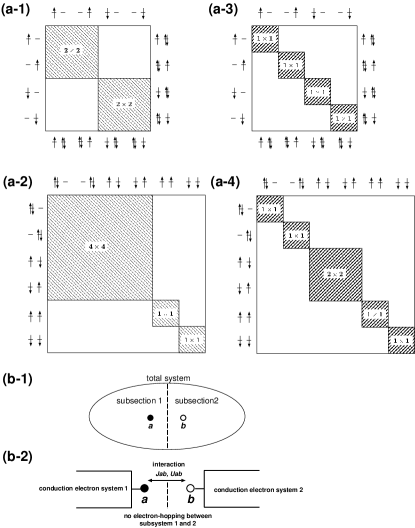
Figure 1: (a)Block matrices of sectors for $N_{Q}=1,3$(a-1) and $N_{Q}=2$(a-2), composing the representation block diagonal matrix of $\rho^{(A)}_{\psi}$ when $\psi$ is an eigenstate of $Q$. Each block matrix is further block diagonalized if $\psi$ is an eigenstate of $S_{z}$ (a-1,2),$S_{z}$ and $\Delta Q$(a-3,4). The pictures placed on the upper and left sides of each matrix show the electron occupancy of the Anderson impurities $a$ and $b$ for $N_{Q}=1$(a-1,3) and $N_{Q}=2$(a-2,4). The electron occupancy of the Anderson impurities $a$ and $b$ for $N_{Q}=3$(a-1,3) is also shown in the pictures placed on the bottom and right sides of each matrix. (b-1) Bisection of all orbitals in total system, where Anderson impurities $a$ and $b$ belong to different subsections. (b-2) Two single impurity Anderson models coupled by magnetic interaction $J_{ab}$ and repulsion $U_{ab}$ between the two impurities without electron transfer, as an example where the bisection shown in (b-1) is useful and natural.

Now, we can easily write down the density operator $\rho^{(ab)}_{\psi}$ as follows;

$$\rho_{\psi}^{(ab)} = \lambda^{(0)}|0\rangle_{ab}{}_{ab}\langle 0|+\sum_{i=a,b,\sigma=\uparrow,\downarrow}\lambda^{(1)}_{i\sigma}|e^{(1)}_{i\sigma}\rangle\langle e^{(1)}_{i\sigma}|$$ (27)

$$\mbox{}+\sum_{i=a,b}\lambda^{(2)}_{i\uparrow,i\downarrow}|e^{(2)}_{i\uparrow,i\downarrow}\rangle\langle e^{(2)}_{i\uparrow,i\downarrow}|+\sum_{\sigma=\uparrow,\downarrow}\lambda^{(2)}_{a\sigma,b\sigma}|e^{(2)}_{a\sigma,b\sigma}\rangle\langle e^{(2)}_{a\sigma,b\sigma}|$$

$$\mbox{}+\sum_{\sigma=\uparrow,\downarrow}\lambda^{(2)}_{a\sigma,b-\sigma}|e^{(2)}_{a\sigma,b-\sigma}\rangle\langle e^{(2)}_{a\sigma,b-\sigma}|$$

$$\mbox{}+C|e^{(2)}_{a\downarrow,b\uparrow}\rangle\langle e^{(2)}_{a\uparrow,b\downarrow}|++\overline{C}|e^{(2)}_{a\uparrow,b\downarrow}\rangle\langle e^{(2)}_{a\downarrow,b\uparrow}|$$

$$\mbox{}+\sum_{\sigma=\uparrow,\downarrow}\lambda^{(3)}_{a\uparrow,a\downarrow,b\sigma}|e^{(3)}_{a\uparrow,a\downarrow,b\sigma}\rangle\langle e^{(3)}_{a\uparrow,a\downarrow,b\sigma}|$$

$$\mbox{}+\sum_{\sigma=\uparrow,\downarrow}\lambda^{(3)}_{a\sigma,b\uparrow,b\downarrow}|e^{(3)}_{a\sigma,b\uparrow,b\downarrow}\rangle\langle e^{(3)}_{a\sigma,b\uparrow,b\downarrow}|$$

$$\mbox{}+\lambda^{(4)}|{\rm F}\rangle_{ab}{}_{ab}\langle{\rm F}|,$$

where

$$|{\rm F}\rangle_{ab} \equiv d^{\dagger}_{a\uparrow}d^{\dagger}_{a\downarrow}d^{\dagger}_{b\uparrow}d^{\dagger}_{b\downarrow}|0\rangle_{ab},$$ (28)

$$\lambda^{(0)} \equiv \langle h_{a\uparrow}h_{a\downarrow}h_{b\uparrow}h_{b\downarrow}\rangle,$$ (29)

$$\lambda^{(1)}_{i\sigma} \equiv \langle n_{i\sigma}h_{i\sigma}h_{i^{c}\uparrow}h_{i^{c}\downarrow}\rangle,$$ (30)

$$\lambda^{(2)}_{i\uparrow,i\downarrow} \equiv \langle n_{i\uparrow}n_{i\downarrow}h_{i^{c}\uparrow}h_{i^{c}\downarrow}\rangle,$$ (31)

$$\lambda^{(2)}_{a\sigma,b\sigma} \equiv \langle n_{a\sigma}n_{b\sigma}h_{a\sigma}h_{b\sigma}\rangle,$$ (32)

$$\lambda^{(2)}_{a\sigma,b-\sigma} \equiv \langle n_{a\sigma}n_{b-\sigma}h_{a\sigma}h_{b-\sigma}\rangle,$$ (33)

$$C \equiv \langle s^{(a)}_{+}s^{(b)}_{-}\rangle,$$ (34)

$$\lambda^{(3)}_{a\uparrow,a\downarrow,b\sigma} \equiv \langle n_{a\uparrow}n_{a\downarrow}n_{b\sigma}h_{b\sigma}\rangle,$$ (35)

$$\lambda^{(3)}_{a\sigma,b\uparrow,b\downarrow} \equiv \langle n_{a\sigma}h_{a\sigma}n_{b\uparrow}n_{b\downarrow}\rangle,$$ (36)

$$\lambda^{(4)} \equiv \langle n_{a\uparrow}n_{a\downarrow}n_{b\uparrow}n_{b\downarrow}\rangle,$$ (37)

and $n_{i\sigma}\equiv d_{i\sigma}^{\dagger}d_{i\sigma}$, $h_{i\sigma}\equiv=I-n_{i,-\sigma}$, $s_{\pm}^{(i)}\equiv d_{i\sigma}^{\dagger}d_{i,-\sigma}$ ($i=a,b,\sigma=\uparrow(+),\downarrow(-)$), $\{e^{(N_{Q})}_{\cdots}\}$ is another representation of the basis (25) classified by the value of $N_{Q}$ and the subindex ($\cdots$) of $e^{(N_{Q})}_{\cdots}$ represents the electron occupancy of the orbitals of Anderson impurity $a$ and $b$.

The entanglement entropy between system $A$ and $B$ is represented as follows;

$$S_{\rm E.E.}^{(ab)} = -\lambda^{(0)}\log\lambda^{(0)}-\sum_{i=a,b,\sigma=\uparrow,\downarrow}\lambda^{(1)}_{i\sigma}\log\lambda^{(1)}_{i\sigma}$$ (38)

$$\mbox{}-\sum_{i=a,b}\lambda^{(2)}_{i\uparrow,i\downarrow}\log\lambda^{(2)}_{i\uparrow,i\downarrow}-\sum_{\sigma=\uparrow,\downarrow}\lambda^{(2)}_{a\sigma,b\sigma}\log\lambda^{(2)}_{a\sigma,b\sigma}$$

$$\mbox{}-\sum_{j=\pm}\lambda^{(2)}_{j}\log\lambda^{(2)}_{j}-\sum_{\sigma=\uparrow,\downarrow}\lambda^{(3)}_{a\uparrow,a\downarrow,b\sigma}\log\lambda^{(3)}_{a\uparrow,a\downarrow,b\sigma}$$

$$\mbox{}-\sum_{\sigma=\uparrow,\downarrow}\lambda^{(3)}_{a\sigma,b\uparrow,b\downarrow}\log\lambda^{(3)}_{a\sigma,b\uparrow,b\downarrow}-\lambda^{(4)}\log\lambda^{(4)}$$

where $\lambda^{(2)}_{\pm}\equiv\frac{\lambda^{(2)}_{a\uparrow,b\downarrow}+\lambda^{(2)}_{a\downarrow,b\uparrow}\pm\sqrt{(\lambda^{(2)}_{a\uparrow,b\downarrow}-\lambda^{(2)}_{a\downarrow,b\uparrow})^{2}+4|C|^{2}}}{2}$.

$S_{\rm E.E.}$ is a function of the following correlation functions; $c^{(1)}_{i\sigma}\equiv\langle n_{i\sigma}\rangle$ , $c^{(2)}_{i\uparrow,i\downarrow}\equiv\langle n_{i\uparrow}n_{i\downarrow}\rangle$ , $c^{(2)}_{a\sigma,b\sigma}\equiv\langle n_{a\sigma}n_{b\sigma}\rangle$ , $c^{(2)}_{a\sigma,b-\sigma}\equiv\langle n_{a\sigma}n_{b-\sigma}\rangle$ , $c^{(3)}_{a\uparrow,a\downarrow,b\sigma}\equiv\langle n_{a\uparrow}n_{a\downarrow}n_{b\sigma}\rangle$ , $c^{(3)}_{a\sigma,b\uparrow,b\downarrow}\equiv\langle n_{a\sigma}n_{b\uparrow}n_{b\downarrow}\rangle$ , $c^{(4)}\equiv\langle n_{a\uparrow}n_{a\downarrow}n_{b\uparrow}n_{b\downarrow}\rangle$ ($i=a,b\ \sigma=\uparrow,\downarrow$) and $|C|$ defined by Eq.(34). To evaluate $S_{\rm E.E.}^{(ab)}$, we need to calculate these 16 correlation functions. This is not an easy calculation, but fortunately the 16 quantities are independent and can be calculated separately, if necessary, in numerical calculations.

As we did in subsection II.1, we consider the stationary problem of $S_{\rm E.E.}^{(ab)}$ and the linear response of $S_{\rm E.E.}^{(ab)}$ to 16 variables. The results of differentiating $S_{\rm E.E.}^{(ab)}$ by these 16 variables is as follows;

$$\frac{\partial S^{(ab)}_{\rm E.E.}}{\partial c^{(1)}_{i\sigma}} = \log\left(\frac{\lambda^{(0)}}{\lambda^{(1)}_{i\sigma}}\right),$$ (39)

$$\frac{\partial S^{(ab)}_{\rm E.E.}}{\partial c^{(2)}_{i\uparrow,i\downarrow}} = \log\left(\frac{\lambda^{(1)}_{i\uparrow}\lambda^{(1)}_{i\downarrow}}{\lambda^{(0)}\lambda^{(2)}_{i\uparrow,i\downarrow}}\right),$$ (40)

$$\frac{\partial S^{(ab)}_{\rm E.E.}}{\partial c^{(2)}_{a\sigma,b\sigma}} = \log\left(\frac{\lambda^{(1)}_{a\sigma}\lambda^{(1)}_{b\sigma}}{\lambda^{(0)}\lambda^{(2)}_{a\sigma,b\sigma}}\right),$$ (41)

$$\frac{\partial S^{(ab)}_{\rm E.E.}}{\partial c^{(2)}_{a\sigma,b-\sigma}} = \log\left(\frac{\lambda^{(1)}_{a\sigma}\lambda^{(1)}_{b-\sigma}}{\lambda^{(0)}\left(\lambda^{(2)}_{+}\right)^{\delta_{\sigma}}\left(\lambda^{(2)}_{-}\right)^{\delta_{-\sigma}}}\right),$$ (42)

$$\frac{\partial S^{(ab)}_{\rm E.E.}}{\partial c^{(3)}_{a\uparrow,a\downarrow,b\sigma}} = \log\left(\frac{\lambda^{(0)}\lambda^{(2)}_{a\uparrow,a\downarrow}\lambda^{(2)}_{a\sigma,b\sigma}\left(\lambda^{(2)}_{+}\right)^{\delta_{-\sigma}}\left(\lambda^{(2)}_{-}\right)^{\delta_{\sigma}}}{\lambda^{(1)}_{a\uparrow}\lambda^{(1)}_{a\downarrow}\lambda^{(1)}_{b\sigma}\lambda^{(3)}_{a\uparrow,a\downarrow,b\sigma}}\right),$$

$$\frac{\partial S^{(ab)}_{\rm E.E.}}{\partial c^{(3)}_{a\sigma,b\uparrow,b\downarrow}} = \log\left(\frac{\lambda^{(0)}\lambda^{(2)}_{b\uparrow,b\downarrow}\lambda^{(2)}_{a\sigma,b\sigma}\left(\lambda^{(2)}_{+}\right)^{\delta_{\sigma}}\left(\lambda^{(2)}_{-}\right)^{\delta_{-\sigma}}}{\lambda^{(1)}_{a\sigma}\lambda^{(1)}_{b\uparrow}\lambda^{(1)}_{b\downarrow}\lambda^{(3)}_{a\sigma,b\uparrow,b\downarrow}}\right),$$

$$\frac{\partial S^{(ab)}_{\rm E.E.}}{\partial c^{(4)}} = \log\left(\frac{\underset{i=a,b,\sigma=\uparrow,\downarrow}{\prod}\left(\lambda^{(1)}_{i\sigma}\right)\underset{\sigma=\uparrow,\downarrow}{\prod}\left(\lambda^{(3)}_{a\uparrow,a\downarrow,b\sigma}\lambda^{(3)}_{a\sigma,b\uparrow,b\downarrow}\right)}{\lambda^{(0)}\underset{i=a,b}{\prod}\left(\lambda^{(2)}_{i\uparrow,i\downarrow}\right)\underset{\sigma=\uparrow,\downarrow}{\prod}\left(\lambda^{(2)}_{a\sigma,b\sigma}\right)\lambda^{(2)}_{+}\lambda^{(2)}_{-}\lambda^{(4)}}\right),$$

$$\frac{\partial S^{(ab)}_{\rm E.E.}}{\partial|C|} = \log\left(\frac{\lambda^{(2)}_{-}}{\lambda^{(2)}_{+}}\right)^{\Delta},$$ (46)

where $\delta_{\pm}\equiv\frac{1}{2}\left(1\pm\frac{\lambda^{(2)}_{a\uparrow,b\downarrow}-\lambda^{(2)}_{a\downarrow,b\uparrow}}{\sqrt{(\lambda^{(2)}_{a\uparrow,b\downarrow}-\lambda^{(2)}_{a\downarrow,b\uparrow})^{2}+4|C|^{2}}}\right)$ and $\Delta\equiv\frac{2|C|}{\sqrt{(\lambda^{(2)}_{a\uparrow,b\downarrow}-\lambda^{(2)}_{a\downarrow,b\uparrow})^{2}+4|C|^{2}}}$. Similar to the results obtained in subsection II.1, the stationary value condition of $S_{\rm E.E.}^{(ab)}$ for each variables gives the relationship among several correlation functions and the logarithm of the displacement of the relation gives the linear response of $S_{\rm E.E.}^{(ab)}$ to each variable. The equal probability conditions obtained from the stationary value conditions of $S_{\rm E.E.}^{(ab)}$ for all variables, written in terms of correlation functions, are $c^{(1)}_{\cdots}=\frac{1}{2}$, $c^{(2)}_{\cdots}=\frac{1}{4}\left(=(\frac{1}{2})^{2}\right)$, $c^{(3)}_{\cdots}=\frac{1}{8}\left(=(\frac{1}{2})^{3}\right)$, $c^{(4)}=\frac{1}{16}\left(=(\frac{1}{2})^{4}\right)$, and $C=0$ , where the maximum value of $S_{\rm E.E.}^{(ab)}$ is $\log(16)$. Again, to have maximum entanglement with $B$, the environmental system of $A$, there must be no correlations inside $A$, and the monogamy of quantum entanglement can be seen.

The degree of entanglement between Anderson impurity $a$ and $b$ can be determined by the mutual information $I$ defined by the following equation;

$$I \equiv D\left(\rho^{(ab)}_{\psi}||\rho^{(a)}_{\psi}\otimes\rho^{(b)}_{\psi}\right)$$ (47)

$$= S^{(a)}_{\rm E.E.}+S_{\rm E.E.}^{(b)}-S_{\rm E.E.}^{(ab)},$$ (48)

where

$$\rho^{(i)}_{\psi} \equiv \langle h_{i\uparrow}h_{i\downarrow}\rangle|0\rangle_{i}{}_{i}\langle 0|+\langle n_{i\uparrow}h_{i\uparrow}\rangle|\uparrow\rangle_{i}{}_{i}\langle\uparrow|$$ (49)

$$\mbox{}+\langle n_{i\downarrow}h_{i\downarrow}\rangle|\downarrow\rangle_{i}{}_{i}\langle\downarrow|+\langle n_{i\uparrow}n_{i\downarrow}\rangle|{\rm F}\rangle_{i}{}_{i}\langle{\rm F}|,$$

$|\sigma\rangle_{i}\equiv d_{i\sigma}^{\dagger}|0\rangle_{i}$, $|{\rm F}\rangle_{i}\equiv d_{i\uparrow}{\dagger}d_{i\downarrow}^{\dagger}|0\rangle_{i}$ and

$$S_{\rm E.E.}^{(i)} = -\langle n_{i\uparrow}n_{i\downarrow}\rangle\log\langle n_{i\uparrow}n_{i\downarrow}\rangle-\langle h_{i\uparrow}h_{i\downarrow}\rangle\log\langle h_{i\uparrow}h_{i\downarrow}\rangle$$

$$\mbox{}-\langle n_{i\uparrow}h_{i\uparrow}\rangle\log\langle n_{i\uparrow}h_{i\uparrow}\rangle-\langle n_{i\downarrow}h_{i\downarrow}\rangle\log\langle n_{i\downarrow}h_{i\downarrow}\rangle$$

($i=a,b$).

The trace distance between $\rho_{\psi}^{(a)}\otimes\rho_{\psi}^{(b)}$ and $\rho_{\psi}^{(ab)}$ is

$$\mbox{}{\rm Tr}\left|\rho_{\psi}^{(a)}\otimes\rho_{\psi}^{(b)}-\rho_{\psi}^{(ab)}\right|$$ (51)

$$= \left|\delta_{ab}\lambda^{(0)}\right|+\sum_{i=a,b,\sigma=\uparrow,\downarrow}\left|\delta_{ab}\lambda^{(1)}_{i\sigma}\right|$$

$$\mbox{}+\sum_{i=a,b}\left|\delta_{ab}\lambda^{(2)}_{i\uparrow,i\downarrow}\right|+\sum_{\sigma=\uparrow,\downarrow}\left|\delta_{ab}\lambda^{(2)}_{a\sigma,b\sigma}\right|$$

$$\mbox{}+\sum_{j=\pm}\left|\delta_{ab}\lambda^{(2)}_{j}\right|+\sum_{\sigma=\uparrow,\downarrow}\left|\delta_{ab}\lambda^{(3)}_{a\uparrow,a\downarrow,b\sigma}\right|$$

$$\mbox{}+\sum_{\sigma=\uparrow,\downarrow}\left|\delta_{ab}\lambda^{(3)}_{a\sigma,b\uparrow,b\downarrow}\right|+\left|\delta_{ab}\lambda^{(4)}\right|,$$

which directly measures the correlation between selected Anderson impurity $a$ and $b$. Here, $\delta_{ab}\lambda^{0}\equiv\lambda^{(0)}-\langle h_{a\uparrow}h_{a\downarrow}\rangle\langle h_{b\uparrow}h_{b\downarrow}\rangle,\cdots$ and $\delta_{ab}\lambda^{(2)}_{\pm}\equiv\frac{\delta_{ab}\lambda^{(2)}_{a\uparrow,b\downarrow}+\delta_{ab}\lambda^{(2)}_{a\downarrow,b\uparrow}\pm\sqrt{(\delta_{ab}\lambda^{(2)}_{a\uparrow,b\downarrow}-\delta_{ab}\lambda^{(2)}_{a\downarrow,b\uparrow})^{2}+4|C|^{2}}}{2}$.

III Results of application to SIAM

In this section, we focus on the simplest non-trivial quantum impurity system, the Single Impurity Anderson Model (SIAM) defined by the following Hamiltonian (52);

$$H \equiv H_{\rm imp}+H_{\rm hyb}+H_{\rm cond},$$ (52)

$$H_{\rm imp} \equiv \sum_{\sigma}\varepsilon_{d}n_{\sigma}+Un_{\uparrow}n_{\downarrow},$$ (53)

$$H_{\rm hyb} \equiv \sum_{\sigma,{\bf k}}V_{\bf k}d_{\sigma}c^{\dagger}_{{\bf k}\sigma}+{\rm h.c.},$$ (54)

$$H_{\rm cond} \equiv \sum_{{\bf k},\sigma}E_{\bf k}c^{\dagger}_{{\bf k}\sigma}c_{{\bf k}\sigma},$$ (55)

where $d_{\sigma}$ annihilates an electron with spin $\sigma$ at the Anderson impurity, characterized by the onsite energy $\varepsilon_{d}$ and the intra-impurity repulsion $U$. Here $n_{\sigma}\equiv d^{\dagger}_{\sigma}d_{\sigma}$ is the number operator of the electron with spin $\sigma$ in the impurity. In the conduction electron system, $c^{\dagger}_{{\bf k}\sigma}$ creates an electron with energy $E_{\bf k}$, spin $\sigma$ and momentum ${\bf k}$, and $V_{\bf k}$ is the hopping integral between the orbital for $({\bf k},\sigma)$-state of the conduction electron system and the orbital of the impurity with spin index $\sigma$. We assume that the hybridization strength $\Delta\equiv\pi\sum_{\bf k}\left|V_{\bf k}\right|^{2}\delta(\omega-E_{\bf k})$ is a constant independent of the frequency $\omega$, and take the Fermi energy $\mu$ to be $\mu=0$. Hence, assuming that the conduction electron system has a flat band structure with half bandwidth $D$ and neglecting the ${\bf k}$-dependence of $V_{\bf k}$, we have $\Delta=\pi V^{2}/(2D)$.

We then study the behavior of the entanglement entropy, mutual information, and relative entropy for the energy eigenstates of this system. In order to calculate these quantities based on the formulas derived in the subsection II.1, it is necessary to calculate the physical quantities (correlation functions) on the Anderson impurity, for which we use the Numerical Renormalization Group (NRG) calculation. In the NRG calculation, the logarithmic discretization parameter $\Lambda$ is set to $\Lambda=2$ and $\Delta/D=0.1$.

Since $[H,Q]=[H,S_{z}]=0$, the discretized Hamiltonian $H_{\rm NRG}$ directly treated in NRG calculation also satisfies $[H_{\rm NRG},Q]=[H_{\rm NRG},S_{z}]=0$. So, the energy eigenstates can be obtained by iterative diagonalization while taking into simultaneous eigenstates of $Q$ and $S_{z}$. Therefore, the formulas derived in the subsection II.1 can be applied to the energy eigenstates of each step $N_{\rm nrg}$ of the NRG calculation.

In the next subsection III.1, we discuss results for the ground state in the low-temperature limit (i.e., the ground state of the NRG fixed point Hamiltonian). In the following subsection III.2, we discuss results for the states corresponding to the high-temperature regime, including the excited states (i.e., the states depending on the NRG step(flow) number $N_{\rm nrg}$).

III.1 Quantum entanglement in ground state of NRG fixed point Hamiltonian

In this subsection, we show the results for the ground state $\psi^{({\rm G})}$ of the NRG fixed point Hamiltonian.

Fig.2 shows the $U$-dependence of the entanglement entropy in the presence of electron-hole symmetry. The horizontal axis is $U/(\pi\Delta)$ on a logarithmic scale and the vertical axis is the entanglement entropy. As the value of $U$ is increased, it can be seen that the entanglement entropy monotonically transitions from $\log(4)$ to $\log(2)$. In the presence of electron-hole symmetry, the entanglement entropy is determined through the value of the correlation function $\langle n_{\uparrow}n_{\downarrow}\rangle$ as shown in Eq.(20). The exact series representation of $\langle n_{\uparrow}n_{\downarrow}\rangle$ with respect to $U$ has been obtained. We confirmed that the calculated results of $\langle n_{\uparrow}n_{\downarrow}\rangle$ using NRG are in good agreement with the exact values for some values of $U$. For $U=0$, the up-spin and down-spin correlations disappear, so the correlation function $\langle n_{\uparrow}n_{\downarrow}\rangle$ takes the maximum value $1/4$ in the case of electron-hole symmetry, resulting in the entanglement entropy of $\log(4)$ of the maximum value. The value of $U$ in the transition region from $\log(4)$ to $\log(2)$ belongs to the strongly correlated region. For typical values of $U$ that can be realized in quantum dot systems etc., the entanglement entropy is considerably larger than $\log(2)$, although it belongs to the transition region. This indicates that, from the quantum entanglement point of view, Anderson impurities should not be easily replaced by quantum spins just because they are in the strongly correlated regime.

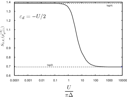
Figure 2: Transition of entanglement entropy with change in $U$

Fig.3 shows the dependence of the entanglement entropy on the onsite energy $\varepsilon_{d}$ for $U/(\pi\Delta)=10$. The horizontal axis is the onsite energy $\varepsilon_{d}$ and the vertical axis is the entanglement entropy, or the average electron number $\langle n\rangle_{\psi^{({\rm G})}}$ in the impurity. It can be seen that the entanglement entropy peaks where the average number of electron changes, and that the entanglement entropy takes values greater than $\log(2)$ around $\langle n\rangle_{\psi^{({\rm G})}}\simeq 1$. To elucidate this feature, we examine the behavior of the correlation functions which are the diagonal component of the density operator.

Figure 3: Entanglement entropy (solid line) and the average electron number in the impurity (dashed line)as functions of $\varepsilon_{d}$

Fig.4(a) shows the $\varepsilon_{d}$-dependence of the correlation functions $\langle n_{\uparrow}n_{\downarrow}\rangle$, $\langle n_{\uparrow}h_{\uparrow}\rangle=\langle n_{\downarrow}h_{\downarrow}\rangle$ and $\langle h_{\uparrow}h_{\downarrow}\rangle$. Note that the spin quantum number ${\mathcal{S}}$ of the ground state we are considering here is zero, so the ground state is magnetic isotropic and $\langle n_{\uparrow}\rangle=\langle n_{\downarrow}\rangle$ holds. The average electron number in the impurity is also shown again in dashed lines for reference in the figure. The correlation function $\langle n_{\uparrow}n_{\downarrow}\rangle$ takes values of approximately 1 in the region where $\langle n\rangle_{\psi^{({\rm G})}}\simeq 2$, and converges monotonically to 0 toward the region where $\langle n\rangle_{\psi^{({\rm G})}}\simeq 0$. Similarly, the correlation function $\langle h_{\uparrow}h_{\downarrow}\rangle$ takes values of approximately 1 in the region where the average hole number in the impurity is approximately 2, and converges monotonically to 0 toward the region where the average hole number in the impurity is approximately 0. On the other hand, the correlation function $\langle n_{\uparrow}h_{\uparrow}\rangle$ has a plateau only in the region where the average particle number and the average hole number in the impurity are approximately 1, and converges to 0 in other regions. The contribution of each correlation function $C$ to the entanglement entropy is expressed as $-C\log(C)$, which has a unimodal peak at $C=1/e$ and is zero at $C=0$ and $1$. Thus, the correlation functions $\langle n_{\uparrow}n_{\downarrow}\rangle$ and $\langle h_{\uparrow}h_{\downarrow}\rangle$ produce peaks in the entanglement entropy in the region where the value of $\langle n\rangle_{\psi^{({\rm G})}}$ changes from 1 to 2 and from 0 to 1, respectively. The correlation function $\langle n_{\uparrow}h_{\downarrow}\rangle$ yields a peak structure in the entanglement entropy in both regions where the value of $\langle n\rangle_{\psi^{({\rm G})}}$ changes from 0 to 1 and from 1 to 2, while even in the region where$\langle n\rangle_{\psi^{({\rm G})}}\simeq 1$, the value of this correlation function is only slightly greater than $1/e$, which yields the value greater than $\log(2)$ for the entanglement entropy. The above results indicate that each peak structure of the entanglement entropy is caused by corresponding two correlation functions ($\langle n_{\uparrow}h_{\uparrow}\rangle=\langle n_{\downarrow}h_{\downarrow}\rangle$ and $\langle n_{\uparrow}n_{\downarrow}\rangle$ or $\langle h_{\uparrow}h_{\downarrow}\rangle$), and that the plateau of the entanglement entropy in the region of the half-filled state is mainly caused by the correlation function $\langle n_{\uparrow}h_{\uparrow}\rangle=\langle n_{\downarrow}h_{\downarrow}\rangle$.

We consider the purity $P(=P(\rho^{(A)}_{\psi}))\equiv{\rm Tr}_{{\mathcal{H}}_{A}}\left(\rho^{(A)}_{\psi}\right)^{2}$, which measures how close the reduced state $\rho^{(A)}_{\psi}$ is to the pure state. In the case of the density operator we are considering now, it is the sum of the squares of the diagonal components. The purity $P$ satisfies $1/4\leq P\leq 1$, where $P=1$ is the pure state and $P=1/4$ is the maximum entropy state. Fig.4(b) shows the $\varepsilon_{d}$-dependence of the purity $P$. The purity $P$ is close to unity for large absolute values of $\varepsilon_{d}$, because the state is closer to the vacuum or fully occupied state, respectively. In the valence fluctuation regime, the purity $P$ decreases due to the contribution of about three states, but in the vicinity of half-filled state, the purity $P$ increases due to the tendency to exclude the vacuum and fully occupied states.

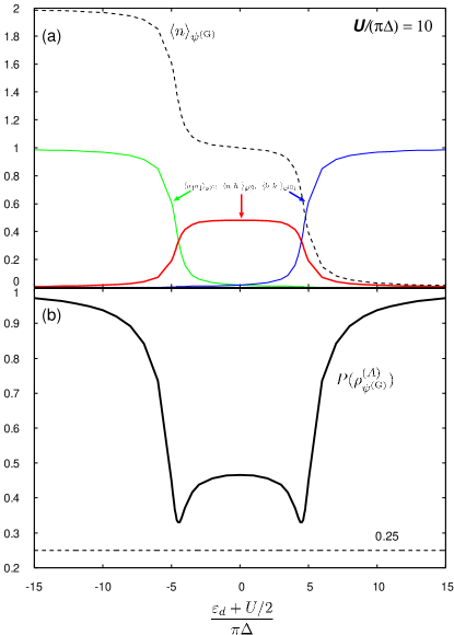
Figure 4: (Color on line)(a)The correlation functions $\langle n_{\uparrow}n_{\downarrow}\rangle$(green solid line), $\langle n_{\uparrow}h_{\downarrow}\rangle$(red solid line), and $\langle h_{\uparrow}h_{\downarrow}\rangle$(blue solid line) as functions of $\varepsilon_{d}$. The $\varepsilon_{d}$-dependence of the average electron number as a reference(dashed line). (b)The purity $P$ as a function of $\varepsilon_{d}$.

To examine the entanglement between up- and down-spin electrons, we will examine the mutual information $I$ defined in Eq.(13). The Fig.5 shows the $\varepsilon_{d}$-dependence of $I$ and also the $\varepsilon_{d}$-dependence of $\delta\equiv\langle n_{\uparrow}\rangle\langle n_{\downarrow}\rangle-\langle n_{\uparrow}n_{\downarrow}\rangle$, one of the quantities measuring electron correlation(deviation from the mean-field approximation). Both $I$ and $\delta$ show rectangle-shaped graphs in the region where $\langle n\rangle_{\psi^{({\rm G})}}\simeq 1$. This is because the mean-field approximation breaks down ($\delta\neq 0$) because the effect of repulsion between up- and down-spin electrons is more pronounced in the region where $\langle n\rangle_{\rm G}\simeq 1$, and there is interdependence where the presence of the electron with one spin in the impurity makes it harder for the electron with the other spin to be present in the impurity, resulting in non zero value of the mutual information $I$ which indicates the interdependence of the up- and down-spin electron states. Although $I$ and $\delta$ are linear independent functions by their definitions and by their graphs shown here, the results indicate that the behavior of $I$ and $\delta$ are positively correlated. From this result, we can say that the mutual information is one of the measures of electron correlation in this case.

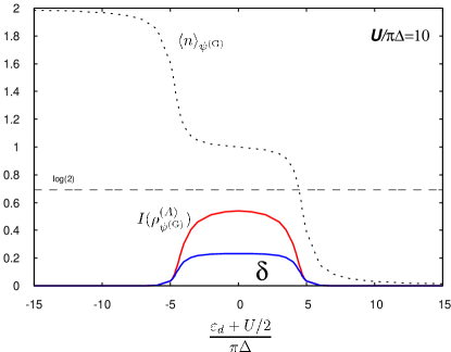
Figure 5: (Color on line)The mutual information $I$(red solid line), and $\delta$(blue solid line) as functions of $\varepsilon_{d}$. The $\varepsilon_{d}$-dependence of the average electron number in the impurity as a reference (dotted line).

Next, we consider the $\varepsilon_{d}$-dependence of entanglement entropy $S_{\rm E.E.}$ and mutual information $I$ when the value of $U/(\pi\Delta)$ is varied. Fig.6 shows the $\varepsilon_{d}$-dependence of $S_{\rm E.E.}$, $I$ and $\langle n\rangle_{\psi^{({\rm G})}}$ for $U/(\pi\Delta)=10,4,2$ and $0$. As for the electron occupancy of the isolated Anderson impurity, it is apparent that the electron number in the impurity is 1 in the interval $-U/2\leq\varepsilon_{d}+U/2\leq U/2$ with interval width $U$. In the system under consideration, the average electron number fluctuates around 1 due to the effect of hybridization with the conduction electron system. Thus, as shown in Fig.6(b), the plateau with $\langle n\rangle\simeq 1$ becomes shorter and more blurred as the value of $U$ decreases. As a result, the correlation function $\langle n_{\uparrow}n_{\downarrow}\rangle$ with a non-zero value in the region where $\langle n\rangle_{\psi^{({\rm G})}}\simeq 2$ and the correlation function $\langle h_{\uparrow}h_{\downarrow}\rangle$ with a non-zero value in the region where $\langle n\rangle_{\psi^{({\rm G})}}\simeq 0$ , viewed as functions of $(\varepsilon_{d}+U/2)/(\pi\Delta)$, move in parallel toward $\varepsilon_{d}+U/2=0$ and overlap each other. Also, the correlation function $\langle n_{\uparrow}h_{\uparrow}\rangle$ goes from a rectangular graph to a unimodal graph. (The two facts above are not illustrated here.) From the above facts, as shown in Fig.6, the side peaks of the entanglement entropy approach each other while getting larger, and the height of the plateau in the half-filling region grows. Also in the case of $U=0$, the side-peak structure disappears and the graph becomes unimodal. Among the three conditions for the maximum entanglement entropy shown in subsection II.1, (A)$\langle n_{\uparrow}\rangle=\langle n_{\downarrow}\rangle$, (B)$\langle n\rangle=1$, and (C)$\langle n_{\uparrow}n_{\downarrow}\rangle=\langle n_{\uparrow}\rangle\langle n_{\downarrow}\rangle$, the condition (A) is always satisfied because the quantum number ${\mathcal{S}}$ of the ground state considered here is ${\mathcal{S}}=0$. The condition (B) is satisfied for $\varepsilon_{d}+U/2=0$ regardless of the value of $U$. The condition (C) is satisfied only when $U=0$ under the previous two conditions. As a result, as shown in Fig.6(a), the entanglement entropy reaches its maximum value $\log(4)$ only when $\varepsilon_{d}+U/2=0$ and $U=0$. Fig.6(b) shows that as the value of $U$ decreases, the region of interdependence between up- and down-spin electrons becomes smaller because the region of average electron number is 1 becomes smaller, as mentioned above, and the degree of interdependence also decreases because the repulsive interaction becomes smaller, resulting in a smaller value of mutual information. Although not shown in the figure, the difference between $\delta$ and $I$ becomes smaller for smaller values of $U$. For $U=0$, $\delta=I\equiv 0$ holds. The above results are consistent with the interpretation that a small value of $U$ leads to low correlation within the Anderson impurity system and a large value of $\Delta$ leads to large hybridization with the conduction electron system, resulting in large entanglement between the Anderson impurity and the conduction electron system.

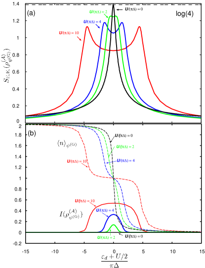
Figure 6: (Color online) Entanglement entropy (a), mutual information and average electron number in the impurity (b) as functions of $\varepsilon_{d}$ for $U/(\pi\Delta)=$10(red), 4(blue), 2(green) and 0(black).

At the end of this subsection, we summarize the results on ground states $\psi^{({\rm G})}$ investigated so far, considering the limit where $U$ is large. Since the quantum number ${\mathcal{S}}$ of the ground state considered so far is ${\mathcal{S}}=0$, the entanglement entropy $S_{\rm E.E.}$ and mutual information $I$ are functions of $\langle n\rangle$ and $\langle n_{\uparrow}n_{\downarrow}\rangle$ because $\langle n_{\uparrow}\rangle=\langle n_{\downarrow}\rangle$. The region of existence of $\langle n\rangle$ and $\langle n_{\uparrow}n_{\downarrow}\rangle$ is the region enclosed by the triangle in $\langle n\rangle$ - $\langle n_{\uparrow}n_{\downarrow}\rangle$ plane in Fig.7(a). The trajectories of $(\langle n\rangle,\langle n_{\uparrow}n_{\downarrow}\rangle)$ for varying $\varepsilon_{d}$ for some vales of $U$ are depicted in Fig.7(a). As $U$ is decreased, the value of the correlation function $\langle n_{\uparrow}n_{\downarrow}\rangle$ increases, so the trajectory shifts to the right, and the trajectory for $U=0$ is given by $\langle n_{\uparrow}n_{\downarrow}\rangle=(\langle n\rangle)^{2}/4$. The region to the the right of this trajectory is the region where the trajectory exists for the case of attractive $U$, which is not addressed in this paper. In the limit $U\to-\infty$, the trajectory asymptotically approaches the right oblique side of the triangle. On the other hand, in the limit $U\to+\infty$, the trajectory asymptotically approaches the left and upper sides of the triangle. Fig.7(b) and (c) show contour plots of the entanglement entropy $S_{\rm E.E.}$ and the mutual information $I$ as functions of $\langle n\rangle$ and $\langle n_{\uparrow}n_{\downarrow}\rangle$, respectively. Considering these figures together, the results shown so far can be clearly understood at a glance. In addition, the following two facts can be understood. When $U$ is large, the entanglement entropy $S_{\rm E.E.}$ plotted as a function of $\varepsilon_{d}$ has two sharp side peaks of $\log(3)$, and has a plateau of $\log(2)$ in the half-filling region. The mutual information $I$ plotted as a function of $\varepsilon_{d}$ asymptotically approaches a rectangular shape with a maximum value of $\log(2)$ in the half-filling region, for the limit $U\to+\infty$.

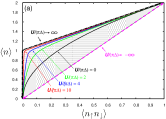
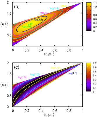
Figure 7: (Color on line) (a) Region of existence of $\langle n\rangle$ and $\langle n_{\uparrow}n_{\downarrow}\rangle$.Trajectories of $(\langle n\rangle,\langle n_{\uparrow}n_{\downarrow}\rangle)$ for varying $\varepsilon_{d}$ for some vales of $U$. (b,c)Contour plots of the entanglement entropy $S_{\rm E.E.}$(b) and the mutual information $I$(c) as functions of $\langle n\rangle$ and $\langle n_{\uparrow}n_{\downarrow}\rangle$.

III.2 Quantum entanglement in energy eigenstates depending on $N_{\rm nrg}$

In this subsection, we investigate the NRG step $N_{\rm nrg}$ dependence of entanglement entropy, mutual information and relative entropy for the energy eigenstates including excited states along the NRG flow.

We first consider the ground state $\psi^{({\rm G},N_{\rm nrg})}$ for each $N_{\rm nrg}$ in the case of the electron-hole symmetric system. Fig.8 shows the $N_{\rm nrg}$-dependence of entanglement entropy $S_{\rm E.E.}$ and mutual information $I$ for $U/(\pi\Delta)=10$, along with the $N_{\rm nrg}$-dependence of $S_{\rm imp}$. Here, $S_{\rm imp}$ is the thermodynamic entropy of the total system minus the thermodynamic entropy of the conduction electron systems, generally with respect to all the quantum impurities in the system (although only one Anderson impurity is in the system considered here). The total energy levels, including the excited states obtained in the NRG calculation contribute to $S_{\rm imp}$ with the weight of the Boltzmann factor for the temperature $T_{N_{\rm nrg}}\equiv\tau\Lambda^{-(N_{\rm nrg}-1)/2}$ determined by $N_{\rm nrg}$, where $\Lambda$ is the NRG discretization parameter and $\tau=O(1)$ is a kind of fitting parameter independent from $N_{\rm nrg}$. Note again that the entanglement entropy or mutual information considered here, on the other hand, is generally a quantity with selectivity determined by the selected quantum impurity and the selected eigenstate of the total system. The graph for $S_{\rm imp}$ in Fig.8 shows that at high temperatures, the four degrees of freedom, the total degrees of freedom of the Anderson impurity appears, but as the temperature decreases, the two degrees of freedom of spin remains, and finally, the Kondo singlet with zero degrees of freedom is formed. On the other hand, the entanglement entropy $S_{\rm E.E.}$ decreases similarly as $S_{\rm imp}$ decreases from $\log(4)$ to $\log(2)$, as seen in Fig.8. This can be interpreted as reflecting a decrease in the contribution of the vacuum state and the fully occupied state to entanglement as the temperature decreases. Fig.8 shows that the entanglement entropy does not change as the temperature is further lowered and the temperature enters the Kondo screening region and becomes even lower. This means that the surviving degrees of freedom contribute to entanglement with the conduction electron system even within the low-temperature limit. The mutual information $I$ increases toward the region where $S_{\rm imp}\simeq\log(2)$ , due to its nature of reflecting the degree of interdependence between the up- and down-electron states, and constant in the low-temperature region thereafter, including the Kondo screening region, as shown Fig.8. The persistence of the interdependence due to the repulsion between up- and down-spin electrons in the impurity in the Kondo screening region and in the lower temperature region thereafter can be understood from the fact that, due to its persistence, the electron in the impurity and conduction electrons form a many-body singlet state(Kondo singlet state) instead of a singlet state in the impurity in that temperature region. We can understand the behavior of these quantities being constant in the Kondo screening region described above from the fact that the spin quantum number ${\mathcal{S}}$ of the ground state of each NRG step $N_{\rm nrg}$ is zero, so that $S_{\rm E.E.}$ and $I$ are represented only by the non-magnetic quantities $\langle n\rangle$ and $\langle n_{\uparrow}n_{\downarrow}\rangle$.

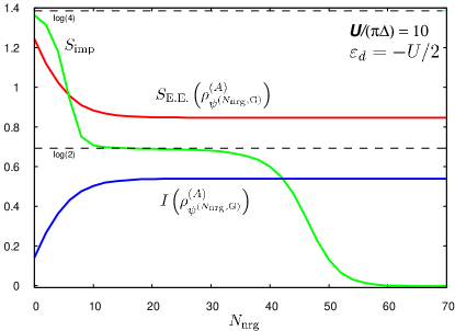
Figure 8: (Color on line) $N_{\rm nrg}$-dependence of $S_{\rm imp}$, $S_{\rm E.E.}\left(\rho^{(A)}_{\psi^{({\rm G},N_{\rm nrg})}}\right)$, and $I\left(\rho^{(A)}_{\psi^{({\rm G},N_{\rm nrg})}}\right)$.

Therefore, to capture the Kondo screening region, we next consider entanglement entropy $S_{\rm E.E.}$, mutual information $I$ and relative entropy $D$ for states with ${\mathcal{S}}\neq 0$(excited states). Since the state with ${\mathcal{S}}\neq 0$ has non-zero ${\mathcal{S}}_{z}$ and the expected value in these states of $s_{z}=\frac{1}{2}(n_{\uparrow}-n_{\downarrow})$ is generally non-zero, $\langle n_{\uparrow}\rangle$ and $\langle n_{\downarrow}\rangle$ in the expressions of $S_{\rm E.E.}$ and $I$ become $\langle n_{\uparrow}\rangle=\langle n\rangle/2+\langle s_{z}\rangle$ and $\langle n_{\downarrow}\rangle=\langle n\rangle/2-\langle s_{z}\rangle$, respectively, and include the magnetic quantity $\langle s_{z}\rangle$. Note that ${\bf S}^{2}$ and $S_{z}$ are operators of the spin magnitude and the $z$-component of the spin for the total system, respectively, and $s_{z}$ is the operator of the $z$-component of the spin of the (selected) Anderson impurity.

The behaviors of the entanglement entropy $S_{\rm E.E.}$ and the mutual information $I$ as functions of $N_{\rm nrg}$ for the lowest energy state $\psi_{\mathcal{Q}}^{({\rm G},N_{\rm nrg})}({\mathcal{S}},{\mathcal{S}}_{z}={\mathcal{S}})$ in states within ${\mathcal{S}}=1/2$ and ${\mathcal{Q}}=\pm 1$ are as follows: The entanglement entropy is indeed found to change in the Kondo screening region. Especially in the case of the electron-hole symmetric systems, it is clearly distinguishable from changes in other regions. However, since the non-magnetic quantities $\langle n\rangle$ and $\langle n_{\uparrow}n_{\downarrow}\rangle$ included in the expression of $S_{\rm E.E.}$ also change, especially in case of systems away from the electron-hole symmetry, they also change outside the Kondo screening region, making the change in the Kondo screening region unclear. As for the mutual information, no clear change is observed in the Kondo screening region because, mathematically, it is a subtraction of two quantities including the magnetic quantities, $S_{\uparrow}+S_{\downarrow}$ and $S_{\rm E.E.}$. The above two results are not illustrated here.

We next consider two states with ${\mathcal{S}}_{z}={\mathcal{S}}$ and ${\mathcal{S}}_{z}=-{\mathcal{S}}$ for the lowest energy state $\psi^{(N_{\rm nrg},\rm G)}_{\mathcal{Q}}({\mathcal{S}},{\mathcal{S}}_{z})$ within ${\mathcal{S}}\neq 0$ and the corresponding appropriate ${\mathcal{Q}}$ for each $N_{\rm nrg}$, and then reduce these two states to the Anderson impurity system and consider the relative entropy $D\left(\rho^{(A)}_{\psi^{(N_{\rm nrg},\rm G)}_{\mathcal{Q}}({\mathcal{S}},{\mathcal{S}})}||\rho^{(A)}_{\psi^{(N_{\rm nrg},\rm G)}_{\mathcal{Q}}({\mathcal{S}},-{\mathcal{S}})}\right)(\equiv D_{{\mathcal{S}}{\mathcal{Q}}}(N_{\rm nrg}))$. For ${\mathcal{S}}\neq 0$, the corresponding appropriate ${\mathcal{Q}}$ retained in our NRG calculation are $({\mathcal{S}},{\mathcal{Q}})=(n/2,\pm 1)$, $(n/2,\pm 3)\ (n=1,3,5)$, $(1/2,\pm 5)$,$(3/2,\pm 5)$, $(m,0),(m,\pm 2)$, $(m,\pm 4)\ (m=1,2)$, $(3,0)$. For each $({\mathcal{S}},{\mathcal{Q}})$ mentioned above, the $N_{\rm nrg}$-dependence of relative entropy $D_{{\mathcal{S}}{\mathcal{Q}}}(N_{\rm nrg})$ are shown in Fig.9. The $N_{\rm nrg}$-dependence of $S_{\rm imp}$ is also shown in the figure again as reference. Here, we have confirmed the following inequalities and equality hold for $N$ in the Kondo screening region; $D_{5/2,\pm 3}(N)>D_{2,\pm 4}(N)$$>D_{3,0}(N)>D_{3/2,\pm 5}(N)>D_{5/2,\pm 1}(N)$$>D_{2,\pm 2}(N)>D_{3/2,\pm 3}(N)$ $>D_{2,0}(N)>D_{3/2,\pm 1}(N)$ $>D_{1,\pm 4}(N)>D_{1/2.\pm 5}(N)$ $>D_{1,\pm 2}(N)>D_{1,0}(N)$ $>D_{1/2,\pm 3}(N)>D_{1/2,\pm 1}(N)$(double sign in same order), $D_{SQ}(N)>D_{SQ^{\prime}}(N)\ (|Q|>|Q^{\prime}|)$, and $D_{S,Q}(N)=D_{S,-Q}(N)$. It is found that the relative entropy of each $({\mathcal{S}},{\mathcal{Q}})$ has a kink between the Kondo screening region and, mostly, for larger values of ${\mathcal{S}}$, $D_{{\mathcal{S}}{\mathcal{Q}}}(N)$ is found to develop a kink toward the end of the Kondo screening region. Therefore, the minimum value of the set of $N_{\rm nrg}$ in which the kink manifests corresponds to the beginning of Kondo screening, and the maximum value of the set corresponds to the end of Kondo screening. In this case, $({\mathcal{S}},{\mathcal{Q}})=(1/2,-1)$ and $(5/2,3)$ respectively gives the minimum and maximum value of the set of $N_{\rm nrg}$.

From the above results, it is found that the Kondo screening region can be detected by looking at the $N_{\rm nrg}$-dependence of the relative entropy $D_{{\mathcal{S}}{\mathcal{Q}}}(N_{\rm nrg})$ for many ${\mathcal{S}}\neq 0$.

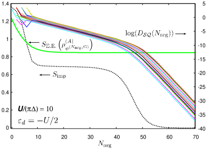
Figure 9: (Color on line) $N_{\rm nrg}$-dependence of $S_{\rm imp}$, $S_{\rm E.E.}\left(\rho^{(A)}_{\psi^{({\rm G},N_{\rm nrg})}}\right)$, and $D_{{\mathcal{S}}{\mathcal{Q}}}(N_{\rm nrg})$ for some values of $({\mathcal{S}},{\mathcal{Q}})$ stated in the main text. See the main text for the shown curves of $D_{{\mathcal{S}}{\mathcal{Q}}}(N_{\rm nrg})$ and values of $({\mathcal{S}},{\mathcal{Q}})$ correspondences.

These features are also seen when the parameters are varied as shown in Fig.10 (For a system away from the electron-hole symmetry shown below, the equation $D_{S,Q}(N)=D_{S,-Q}(N)$ does not hold and the inequality $D_{S,Q}(N)>D_{S,-Q}(N)\ (Q>0)$ holds.). Fig.10 shows that the $N_{\rm nrg}$-dependence of the entangle entropy $S_{\rm E.E.}$ of the ground state for each $N_{\rm nrg}$, the relative entropy $D_{{\mathcal{S}}{\mathcal{Q}}}(N_{\rm nrg})$ for $({\mathcal{S}},{\mathcal{Q}})=(1/2,-1)$ and $(5/2,3)$, and the impurity entropy $S_{\rm imp}$, for a electron-hole symmetric system with smaller value of $U$ and a system away from the electron-hole symmetry. The Fig.10 shows that the transition regions from $\log(4)$ to $\log(2)$ and the Kondo screening regions change from the previous results due to the change in the value of $U$ and the deviation from the electron-hole symmetry, and correspondingly, the regions of decreasing entanglement entropy and the regions where kinks appear in the relative entropy, respectively.

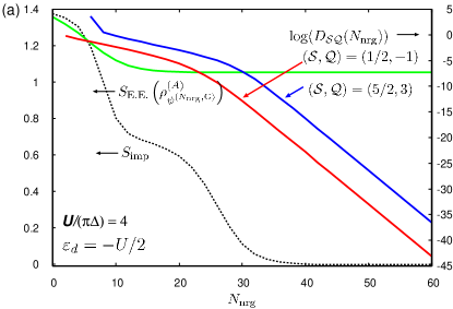
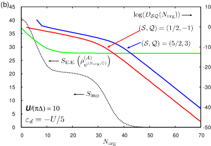
Figure 10: (Color on line) $N_{\rm nrg}$-dependence of $S_{\rm imp}$, $S_{\rm E.E.}\left(\rho^{(A)}_{\psi^{({\rm G},N_{\rm nrg})}}\right)$, and $D_{{\mathcal{S}}{\mathcal{Q}}}(N_{\rm nrg})$ for $({\mathcal{S}},{\mathcal{Q}})=(1/2.-1)$ and $(5/2,3)$. (a)A electron-hole symmetric system with smaller value of $U$,(b) A system away from the electron-hole symmetry.

IV Conclusion

In order to formulate the distribution of quantum entanglement on quantum impurities and quantum entanglement in quantum impurity pair in the system, for states of interest in quantum impurity systems, we have considered quantum entanglement between a subsystem consisting of one or two quantum impurities arbitrarily selected from the system and its complement, the environmental system. For this purpose, the pure state of interest has been reduced to the subsystem consisting of selected quantum impurities to obtain the density operator, and quantum informative quantities such as entanglement entropy have been calculated. The pure states of interest in quantum impurity systems are often simultaneous eigenstates of physical quantities such as total particle number $Q$, total spin $S_{z}$ ($\Delta Q$), etc. (and often also energy eigenstates of the system). It has been shown that the density operator is diagonal or almost diagonal in this case. As a result, we have shown that entanglement entropy, mutual information, and relative entropy are given by relatively simple formulas, and that these quantities can be expressed in terms of expectation values of physical quantities on the selected quantum impurities and their correlation functions which can be calculated independently of each other. As we have demonstrated, these expectation values and correlation functions can be calculated with high precision using NRG. It should also be denoted that, apart from their usefulness and possibility of highly accurate numerical calculations, as can be seen within the derivation process, the equations derived here can be applied to systems other than quantum impurity systems(e.g.,Hubbard model, periodic Anderson model, etc.).

Numerical evaluation of these formulas has been performed for SIAM, where the most basic Kondo effect is manifested, using NRG calculation. The SIAM has only one Anderson impurity to choose from, but if that one Anderson impurity system is regarded as a composite system of two spinless Anderson impurity systems, one can choose two of them from the system. This can be regarded as a simplified template for the set up in the subsection II.2 that discusses the case where the subsystem consists of two quantum impurities. In fact, we have also calculated the mutual information between the up- and down-spin electron systems from this perspective. As a result, we have confirmed that the behavior of SIAM from the high temperature region to the low temperature region including the Kondo screening region can be captured with the quantum informative quantities. In this process, we have calculated anew the magnetization $s_{z}$ of the impurity in non zero $S_{z}$ state in SIAM under zero magnetic field with SU(2) symmetry, a calculation not previously reported. (The quantity $s_{z}$ belongs to the representation of $L=1$ in the representation theory of SU(2), so the computational complexity in NRG is larger than that of the quantity belonging to $L=0$($n,n_{\uparrow}n_{\downarrow}$ etc.) or $L=1/2$( the creation operator of the discretized conduction electron in NRG etc.), which has been repeatedly calculated hitherto). We have also analyzed separately all excited states with high $S$ retained in the NRG calculation and have decomposed the Kondo screening process along these states. These are new findings for SIAM itself.

In summary, the method proposed in this paper is expected to elucidate the quantum entanglement of states of various multiple quantum impurity systems beyond SIAM. Using the method described in the subsection II.2, it is possible to analyze the entanglement between the two selected quantum impurities. This is expected to provide a better understanding of the quantum entanglement in the state of interest than the analysis for a single choice of quantum impurity(even without the assumption that the state of interest is an eigenstate of $\Delta Q$, the number of independent physical quantities to be calculated is 26 for systems without any symmetry which,while computationally time-consuming is not impractical). In particular, when the state of interest is further an eigenstate of $\Delta Q$, the method is computationally more accessible. One of the future taska is to apply these to investigations of the duality between itinerant and localized nature in the new (topological) local Fermi liquids.

- (1) For example, see a very recent paperD’Emidio et al. (2024) on this topics and the bibliography in a review paperLaflorencie (2016).
- Costi and H. (2003) T. A. Costi and M. R. H., Phys.Rev.A 68, 034301 (2003).
- He and Millis (2017) Z. He and A. J. Millis, Phys.Rev.B 96, 085107 (2017).
- He and Millis (2019) Z. He and A. J. Millis, Phys.Rev.B 99, 205138 (2019).
- Kohn and Santoro (2022) L. Kohn and G. E. Santoro, J. Stat. Mech. 2022, 063102 (2022).
- Dehollain et al. (2020) J. P. Dehollain, U. Mukhopadhyay, V. P. Michal, Y. Wang, B. Wunsch, C. Reichl, W. Wegscheider, M. S. Rudner, E. Demler, and L. M. K. Vandersypen, Nature 579, 528 (2020).
- Goldhaber-Gordon et al. (1998a) D. Goldhaber-Gordon, H. Shtrikman, D. Mahalu, D. Abusch-Magder, U. Meirav, and M. Kastner, Nature 391, 156 (1998a).
- Goldhaber-Gordon et al. (1998b) D. Goldhaber-Gordon, J. Göres, M. A. Kastner, H. Shtrikman, D. Mahalu, and U. Meirav, Phys. Rev. Lett. 81, 5225 (1998b).
- Potok et al. (2007) R. Potok, I. Rau, H. Shtrikman, Y. Oreg, and D. Goldhaber-Gordon, Nature 446, 167 (2007).
- Cronenwett et al. (1998) S. M. Cronenwett, T. H. Oosterkamp, and L. P. Kouwenhoven, Science 281, 540 (1998).
- Jeong et al. (2001) H. Jeong, A. M. Chang, and M. R. Melloch, Science 293, 2221 (2001).
- Iftikhar et al. (2015) Z. Iftikhar, S. Jezouin, A. Anthore, U. Gennser, F. Parmentier, A. Cavanna, and F. Pierre, Nature 526, 233 (2015).
- Sasaki et al. (2000) S. Sasaki, S. De Franceschi, J. Elzerman, W. Van der Wiel, M. Eto, S. Tarucha, and L. Kouwenhoven, Nature 405, 764 (2000).
- Kobayashi et al. (2010) T. Kobayashi, S. Tsuruta, S. Sasaki, T. Fujisawa, Y. Tokura, and T. Akazaki, Phys. Rev. Lett. 104, 036804 (2010).
- Lieb and Mattis (1962) E. Lieb and D. Mattis, J. Math. Phys. 3, 749 (1962).
- Lieb (1989) E. H. Lieb, Phys. Rev. Lett. 62, 1201 (1989).
- Nagaoka.Y (1965) Nagaoka.Y, Solid State Commun. 3, 409 (1965).
- Nagaoka.Y (1966) Nagaoka.Y, Phys.Rev. 147, 392 (1966).
- Tasaki (2020) H. Tasaki, Physics and Mathematics of Quantum Many-Body Systems (Springer International Publishing, 2020).
- Buterakos and Das Sarma (2019) D. Buterakos and S. Das Sarma, Phys. Rev. B 100, 224421 (2019).
- Tokuda and Nishikawa (2022) M. Tokuda and Y. Nishikawa, Phys.Rev.B 105, 195120 (2022).
- Numata et al. (2009) T. Numata, Y. Nisikawa, A. Oguri, and H. A. C., Phys. Rev. B 80, 155330 (2009).
- Krishna-murthy et al. (1980) H. R. Krishna-murthy, J. W. Wilkins, and K. G. Wilson, Phys. Rev. B 21, 1044 (1980).
- Nisikawa and Oguri (2006) Y. Nisikawa and A. Oguri, Phys. Rev. B 73, 125108 (2006).
- Oguri et al. (2005) A. Oguri, Y. Nisikawa, and A. C. Hewson, J. Phys. Soc. Jap. 74, 2554 (2005).
- Yi et al. (2020) G.-Y. Yi, C. Jiang, L.-L. Zhang, S.-R. Zhong, H. Chu, and W.-J. Gong, Phys. Rev. B 102, 085418 (2020).
- Chung et al. (2008) C.-H. Chung, G. Zarand, and P. Wölfle, Phys. Rev. B 77, 035120 (2008).
- Cornaglia and Grempel (2005) P. S. Cornaglia and D. R. Grempel, Phys. Rev. B 71, 075305 (2005).
- Granger et al. (2005) G. Granger, M. A. Kastner, I. Radu, M. P. Hanson, and A. C. Gossard, Phys. Rev. B 72, 165309 (2005).
- Bomze et al. (2010) Y. Bomze, I. Borzenets, H. Mebrahtu, A. Makarovski, H. U. Baranger, and G. Finkelstein, Phys. Rev. B 82, 161411 (2010).
- Curtin et al. (2018) O. J. Curtin, Y. Nishikawa, A. C. Hewson, and C. D. J. G., J.Phys.Commun. 2, 031001 (2018).
- Nishikawa et al. (2018) Y. Nishikawa, O. Curtin, A. C. Hewson, and D. J. G. Crow, Phys.Rev.B 98, 104419 (2018).
- Blesio et al. (2018) G. G. Blesio, L. O. Manuel, P. Roura-Bas, and A. A. Aligia, Phys.Rev.B 98, 195435 (2018).
- Žitko et al. (2021) R. Žitko, G. G. Blesio, L. O. Manuel, and A. A. A., Nature Commun. 12, 6027 (2021).
- Blesio and A. (2023) G. G. Blesio and A. A. A., Phys.Rev.B 108, 045113 (2023).
- Blesio et al. (2023) G. G. Blesio, R. Žitko, L. O. Manuel, and A. A. A., SciPost Phys 14, 042 (2023).
- Coffman et al. (2000) V. Coffman, J. Kundu, and W. Wotters, Phys.Rev.A 61, 052306 (2000).
- Osborne and Verstraete (2006) T. J. Osborne and F. Verstraete, Phys.Rev.Lett. 96, 220503 (2006).
- Umegaki (1962) H. Umegaki, Koudai Math. Semi. Rep. 14, 59 (1962).
- D’Emidio et al. (2024) J. D’Emidio, R. Orus, N. Laflorencie, and F. de Juan, Phys.Rev.Lett. 132, 076502 (2024).
- Laflorencie (2016) N. Laflorencie, Physics Reports 646, 1 (2016).