Integrable semi-discretization for a modified Camassa-Holm equation with cubic nonlinearity

Abstract

In the present paper, an integrable semi-discretization of the modified Camassa–Holm (mCH) equation with cubic nonlinearity is presented. The key points of the construction are based on the discrete Kadomtsev-Petviashvili (KP) equation and appropriate definition of discrete reciprocal transformations. First, we demonstrate that these bilinear equations and their determinant solutions can be derived from the discrete KP equation through Miwa transformation and some reductions. Then, by scrutinizing the reduction process, we obtain a set of semi-discrete bilinear equations and their general soliton solutions in the Gram-type determinant form. Finally, we obtain an integrable semi-discrete analog of the mCH equation by introducing dependent variables and discrete reciprocal transformation. It is also shown that the semi-discrete mCH equation converges to the continuous one in the continuum limit.

1 Introduction

In this paper, we are concerned with integrable discretization of the following modified Camassa-Holm (mCH) equation with cubic nonlinearity

$$m_{t}+[m(u^{2}-u_{x}^{2})]_{x}=0,\quad m=u-u_{xx}.$$ (1)

Here $u=u(x,t)$ is a real valued function of time $t$ and a spatial variable $x$, and the subscripts $x$ and $t$ appended to $m$ and $u$ denote partial differentiation. It was firstly proposed by Fuchssteiner and Fokas in 1981 (see (32) of Ref. [1]) as a special case of a more general system. Then it appeared in the papers of Fokas [2], Fuchssteiner [3], Olver and Rosenau [4], and later was rediscovered by Qiao [5, 6]. The mCH equation (1) has attracted considerable attention over the past two decades due to its rich mathematical structure and solutions. It has been extensively investigated in various areas, including well-posedness, regularization, the Cauchy problem, the Riemann-Hilbert problem, long-time asymptotics, and the Liouville correspondence with the modified Korteweg-de Vries (KdV) equation [14, 15, 16, 7, 8, 9, 10, 11, 13, 12]. Matsuno presented a compact parametric representation of the smooth bright multisoliton solutions for the mCH equation via the Hirota’s bilinear method [17], while Hu et al. derived its Gram-type determinant solution from the extended Kadomtsev–Petviashvili (KP) hierarchy with negative flow [18]. Several groups also constructed the smooth soliton solutions through Darboux transformation/Bäcklund transformation method [19, 21, 20] and Lie algebraic approach [22]. In [23], the wave-breaking problem and the existence of single and multi-peakon solutions to the mCH equation have been discussed. Recently, Chang et al. have investigated the Lax integrability and the conservative peakon solutions in a series of work [24, 25, 26]. Gao et al. studied the patched peakon weak solution [27], and the conservative sticky peakons [28]. Other related problem such as blow-up phenomena and the stability including the orbital stability have been studied by several authors [29, 30, 31, 32].

Recently, research on discrete integrable systems has garnered significant attention due to its connections to several other fields, including random matrices, quantum field theory, numerical algorithms, orthogonal and biorthogonal polynomials, and random matrices [33]. There are far fewer instances of discrete integrable systems and analytical tools available as compared to continuous integrable systems. On the other hand, discrete integrable systems are seen to be more basic and universal than continuous ones [34]. The authors have conducted extensive research in finding integrable discretizations of soliton equations, including the short pulse equation [35, 36], (2+1)-dimensional Zakharov equation[37], the Camassa-Holm (CH) equation [38, 39], the Degasperis-Procesi equaiton [40], the generalized sine-Gordon equation [41, 42] and the mCH equation with cubic nonlinearity and linear dispersion term [43] via Hirota’s bilinear method.

It should be commented that there exists a mCH equation with cubic nonlinearity and linear dispersion term

$$m_{t}+[m(u^{2}-u_{x}^{2})]_{x}+2\kappa^{2}u_{x}=0,\quad m=u-u_{xx},$$ (2)

whose bilinear equations are totally different from those of Eq. (1). The mCH equation with linear dispersion term were derived in [44] and also in [43] as the reduction of the negative flow of the deformed KdV hierarchy. Although in [43] we have proposed an integrable semi-discretization of the mCH equation with linear dispersion term, i.e., Eq. (2), to the best of our knowledge, integrable discrete analogues of Eq. (1) (the mCH equation without linear dispersion term) have not been reported yet. There are mainly two challenging points in the construction. Firstly, bilinear equations of the mCH equation (1) are reduced from the extended KP hierarchy with negative flow. The non-original location of one of the poles presents a challenge in constructing its discrete analogue. Secondly, as shown in Section 3, we have to define a second discrete counterpart for the same continuous variable in order to obtain an explicit form of the semi-discrete mCH equation. Hence, it is a natural but definitely not a trivial problem to generate a semi-discrete version for the mCH equation (1).

In this paper, upon introducing appropriate Miwa transformation, we derive successfully the two sets bilinear mCH equation from the discrete KP equation. As a byproduct, integrable semi-discrete bilinear mCH equation and the corresponding Gram-type determinant solutions are obtained. Under the discrete reciprocal transformation and dependent variable transformation, an integrable semi-discrete analog of the mCH equation is given.

The outline of the paper is as follows. In section 2, we review the bilinear forms and determinant solutions of the mCH equation, which can be reduced from the discrete KP equation and its $\tau$-function through a series of transformations including Miwa transformation. In section 3, by scrutinizing the process in deriving the bilinear mCH equation from the discrete KP equation, we propose semi-discrete analogues of bilinear mCH equations. Based on these discrete bilinear equations, we construct an integrable semi-discrete mCH equation and present its $N$-soliton solutions. Section 4 is devoted to a brief summary and discussion.

2 From the discrete KP equation to the modified Camassa-Holm equation

In this section, we first review the results in [18] about the bilinear form of the mCH equation. The mCH equation (1) can be transformed into the following bilinear equations

$$\left(2D_{\tau}D_{y}^{2}+2D_{\tau}D_{y}-4D_{y}\right)g\cdot f=0,$$ (3)

$$\left(D_{y}^{2}+D_{y}\right)g\cdot f=0,$$ (4)

through the reciprocal transformation

$$x=y+\tau+2\ln\frac{g}{f},$$ (5)

$$t=\tau,$$ (6)

and the dependent variable transformation

$$u=1-(\ln fg)_{y\tau},$$ (7)

where $D_{x}$ is the Hirota D-operator defined by

$$D_{x}^{n}f\cdot g=\left(\frac{\partial}{\partial x}-\frac{\partial}{\partial y}\right)^{n}f(x)g(y)|_{y=x}.$$

Next, we give a lemma regarding bilinear equations of the mCH equation (1) and show the correspongding reductions.

Lemma 2.1.

The following bilinear equations

$$\left(D_{x_{1}}^{2}-D_{x_{2}}+2cD_{x_{1}}\right)\tau_{n}\cdot\tau_{n+1}=0,$$ (8)

$$\left(D_{x_{-1}}\left(D_{x_{1}}^{2}-D_{x_{2}}+2cD_{x_{1}}\right)-4D_{x_{1}}\right)\tau_{n}\cdot\tau_{n+1}=0,$$ (9)

admit the Gram-type determinant solutions

$$\tau_{n}=\det\limits_{1\leqslant i,j\leqslant N}\left(m_{ij}^{(n)}\right),$$

where the matrix element is defined as

$$m_{ij}^{(n)}=c_{ij}+\frac{1}{p_{i}+q_{j}}\left(-\frac{p_{i}-c}{q_{j}+c}\right)^{-n}e^{\xi_{i}+\eta_{j}},$$

$$\xi_{i}=p_{i}x_{1}+p_{i}^{2}x_{2}+\frac{1}{p_{i}-c}x_{-1}+\xi_{i0},$$

$$\eta_{j}=q_{j}x_{1}-q_{j}^{2}x_{2}+\frac{1}{q_{j}+c}x_{-1}+\eta_{j0},$$

and $c_{ij},p_{i},q_{j},\xi_{i0},\eta_{j0},c$ are constants.

Proof.

The discrete Kadomtsev-Petviashvili (dKP) equation, or the Hirota-Miwa (HM) equation,

$$a_{1}\left(a_{2}-a_{3}\right)\tau\left(k_{1}+1,k_{2},k_{3}\right)\tau\left(k_{1},k_{2}+1,k_{3}+1\right)$$

$$+a_{2}\left(a_{3}-a_{1}\right)\tau\left(k_{1},k_{2}+1,k_{3}\right)\tau\left(k_{1}+1,k_{2},k_{3}+1\right)$$

$$+a_{3}\left(a_{1}-a_{2}\right)\tau\left(k_{1},k_{2},k_{3}+1\right)\tau\left(k_{1}+1,k_{2}+1,k_{3}\right)=0,$$ (10)

was proposed independently by Hirota [45] and Miwa [46] in early 1980s. It is known that the discrete KP equation admits a general solution in terms of the following Gram-type determinant [47]:

$$\tau(k_{1},k_{2},k_{3})=\left|m_{ij}\right|=\left|c_{ij}+\frac{1}{p_{i}+q_{j}}\prod_{l=1}^{3}\left(\frac{1-a_{l}p_{i}}{1+a_{l}q_{j}}\right)^{-k_{l}}\right|_{1\leqslant i,j\leqslant N}.$$ (11)

Notice that the element in Gram-type solution (11) of the discrete KP equation (10) can be rewritten as

$$m_{ij}= c_{ij}+\frac{1}{p_{i}+q_{j}}\left(\frac{1-a_{1}p_{i}}{1+a_{1}q_{j}}\right)^{-k_{1}}\left(\frac{1-a_{2}p_{i}}{1+a_{2}q_{j}}\right)^{-k_{2}}\left(\frac{1-a_{3}p_{i}}{1+a_{3}q_{j}}\right)^{-k_{3}}$$

$$= c_{ij}+\frac{1}{p_{i}+q_{j}}\left(-\frac{p_{i}}{q_{j}}\right)^{-k_{3}}\left(\frac{1-a_{1}p_{i}}{1+a_{1}q_{j}}\right)^{-k_{1}}\left(\frac{1-a_{2}p_{i}}{1+a_{2}q_{j}}\right)^{-k_{2}}\left(\frac{1-a_{3}^{-1}p_{i}^{-1}}{1+a_{3}^{-1}q_{j}^{-1}}\right)^{-k_{3}}$$

$$= c_{ij}+\frac{1}{\tilde{p}_{i}+\tilde{q}_{j}}\left(-\frac{\tilde{p}_{i}-c}{\tilde{q}_{j}+c}\right)^{-k_{3}}\left(\frac{1-b_{1}\tilde{p}_{i}}{1+b_{1}\tilde{q}_{j}}\right)^{-k_{1}}\left(\frac{1-b_{2}\tilde{p}_{i}}{1+b_{2}\tilde{q}_{j}}\right)^{-k_{2}}\left(\frac{1-dp_{i}^{-1}}{1+dq_{j}^{-1}}\right)^{-k_{3}},$$

where $\tilde{p}_{i}=p_{i}+c,\tilde{q}_{i}=q_{i}-c,b_{1}^{-1}=a_{1}^{-1}+c,b_{2}^{-1}=a_{2}^{-1}+c,d=a_{3}^{-1}$. We then drop the tilde for simplicity. Let $k_{3}=n=m$, then the discrete KP equation becomes the discrete deformed modified KP equation

$$\left(d-b_{2}^{-1}+c\right)\tau_{n}\left(k_{1}+1,k_{2},m\right)\tau_{n+1}\left(k_{1},k_{2}+1,m+1\right)$$

$$+\left(b_{1}^{-1}-c-d\right)\tau_{n}\left(k_{1},k_{2}+1,m\right)\tau_{n+1}\left(k_{1}+1,k_{2},m+1\right)$$

$$+\left(b_{2}^{-1}-b_{1}^{-1}\right)\tau_{n+1}\left(k_{1},k_{2},m+1\right)\tau_{n}\left(k_{1}+1,k_{2}+1,m\right)=0.$$ (12)

Applying Miwa transformation

$$x_{1}=\sum\limits_{j=1}^{2}k_{j}b_{j},\ x_{2}=\frac{1}{2}\sum\limits_{j=1}^{2}k_{j}b_{j}^{2},\cdots,x_{k}=\frac{1}{k}\sum_{j=1}^{2}k_{j}b_{j}^{k},$$

$$x_{-1}=md,\ x_{-1}=\frac{1}{2}md^{2},\cdots,x_{-k}=\frac{1}{k}md^{k},$$

and taking $b_{j}\rightarrow 0,\ j=1,2$ and $d\rightarrow 0$, we obtain an infinite number of bilinear equations:

$$\sum_{K,L,M}\left(d-b_{2}^{-1}+c\right)b_{1}^{K}b_{2}^{L}d^{M}p_{K}\left(\frac{1}{2}\tilde{D}_{+}\right)p_{L}\left(-\frac{1}{2}\tilde{D}_{+}\right)p_{M}\left(-\frac{1}{2}\tilde{D}_{-}\right)\tau_{n}\cdot\tau_{n+1}$$

$$+\sum_{K,L,M}\left(b_{1}^{-1}-c-d\right)b_{1}^{K}b_{2}^{L}d^{M}p_{K}\left(-\frac{1}{2}\tilde{D}_{+}\right)p_{L}\left(\frac{1}{2}\tilde{D}_{+}\right)p_{M}\left(-\frac{1}{2}\tilde{D}_{-}\right)\tau_{n}\cdot\tau_{n+1}$$

$$+\sum_{K,L,M}\left(b_{2}^{-1}-b_{1}^{-1}\right)b_{1}^{K}b_{2}^{L}d^{M}p_{K}\left(-\frac{1}{2}\tilde{D}_{+}\right)p_{L}\left(\frac{1}{2}\tilde{D}_{+}\right)p_{M}\left(\frac{1}{2}\tilde{D}_{-}\right)\tau_{n}\cdot\tau_{n+1}=0,$$

where

$$\tilde{D}_{+}=\left(D_{x_{1}},\frac{1}{2}D_{x_{2}},\cdots,\frac{1}{n}D_{x_{n}}\right),\ \tilde{D}_{-}=\left(D_{x_{-1}},\frac{1}{2}D_{x_{-2}},\cdots,\frac{1}{n}D_{x_{-n}}\right).$$

At the order of $b_{1}^{0}b_{2}^{0}d^{0}$, we have

$$\left(-p_{1}\left(\frac{1}{2}\tilde{D}_{+}\right)p_{1}\left(-\frac{1}{2}\tilde{D}_{+}\right)+cp_{1}\left(\frac{1}{2}\tilde{D}_{+}\right)+p_{2}\left(-\frac{1}{2}\tilde{D}_{+}\right)\right.$$

$$\left.-cp_{1}\left(-\frac{1}{2}\tilde{D}_{+}\right)+p_{1}^{2}\left(\frac{1}{2}\tilde{D}_{+}\right)-p_{2}\left(\frac{1}{2}\tilde{D}_{+}\right)\right)\tau_{n}\cdot\tau_{n+1}=0,$$ (13)

which gives equation (8).

At the order of $b_{1}^{1}b_{2}^{0}d^{1}$, we have

$$\left(p_{1}\left(\frac{1}{2}\tilde{D}_{+}\right)-p_{1}\left(\frac{1}{2}\tilde{D}_{+}\right)p_{1}\left(-\frac{1}{2}\tilde{D}_{+}\right)p_{1}\left(-\frac{1}{2}\tilde{D}_{-}\right)+cp_{1}\left(\frac{1}{2}\tilde{D}_{+}\right)p_{1}\left(-\frac{1}{2}\tilde{D}_{-}\right)\right.$$

$$+p_{2}\left(-\frac{1}{2}\tilde{D}_{+}\right)p_{1}\left(-\frac{1}{2}\tilde{D}_{-}\right)-cp_{1}\left(-\frac{1}{2}\tilde{D}_{+}\right)p_{1}\left(-\frac{1}{2}\tilde{D}_{-}\right)-p_{1}\left(-\frac{1}{2}\tilde{D}_{+}\right)$$

$$\left.+p_{1}^{2}\left(\frac{1}{2}\tilde{D}_{+}\right)p_{1}\left(-\frac{1}{2}\tilde{D}_{-}\right)-p_{2}\left(\frac{1}{2}\tilde{D}_{+}\right)p_{1}\left(-\frac{1}{2}\tilde{D}_{-}\right)\right)\tau_{n}\cdot\tau_{n+1}=0,$$ (14)

which leads to equation (9). The proof is complete. ∎

If we impose the constraints

$$p_{i}=q_{i},\ c_{ij}=\delta_{ij},$$

one can verify that $\partial_{x_{2}}\tau_{n}=0$. Setting $\tau_{1}=g,\ \tau_{0}=f$, we obtain from (8)-(9) the following bilinear equations

$$\left(D_{x_{1}}^{2}+2cD_{x_{1}}\right)f\cdot g=0,$$ (15)

$$\left(D_{x_{-1}}\left(D_{x_{1}}^{2}+2cD_{x_{1}}\right)-4D_{x_{1}}\right)f\cdot g=0.$$ (16)

Furthermore, by setting $x_{1}=y,\ x_{-1}=\frac{\tau}{2}$ and $c=-\frac{1}{2}$, we arrive at the bilinear equations of the mCH equation (3)-(4). Thus $\tau$-functions $f$ and $g$ admit the following Gram-type determinant form

$$\tau_{n}=\left|\delta_{ij}+\frac{1}{p_{i}+p_{j}}\left(-\frac{2p_{i}+1}{2p_{j}-1}\right)^{-n}e^{\xi_{i}+\eta_{j}}\right|,$$ (17)

$$\xi_{i}=p_{i}y+\frac{1}{2p_{i}+1}t+\xi_{i0},$$ (18)

$$\eta_{j}=p_{j}y+\frac{1}{2p_{i}-1}t+\xi_{i0},$$ (19)

with $g=\tau_{1},\ f=\tau_{0}$.

3 Integrable semi-discretization of the modified Camassa-Holm equation

In this section, we aim to construct the integrable spatial discretization of the mCH equation. To this end, we shall first derive semi-discrete analogs of the bilinear equations (3)-(4). Subsequently, in Subsection 3.2, we construct an integrable semi-discrete mCH equation.

3.1 From discrete KP equation to the semi-discrete analog of (8) and (9)

Lemma 3.1.

The discrete KP equation (10) generates the following bilinear equations

$$\left(-b_{2}^{-1}+c\right)\tau_{n}\left(k+1,l\right)\tau_{n+1}\left(k,l+1\right)+\left(b_{1}^{-1}-c\right)\tau_{n}\left(k,l+1\right)\tau_{n+1}\left(k+1,l\right)$$

$$+\left(b_{2}^{-1}-b_{1}^{-1}\right)\tau_{n}\left(k+1,l+1\right)\tau_{n+1}\left(k,l\right)=0,$$ (20)

$$\left(-b_{2}^{-1}+c\right)D_{-1}\tau_{n}\left(k+1,l\right)\cdot\tau_{n+1}\left(k,l+1\right)+\left(b_{1}^{-1}-c\right)D_{-1}\tau_{n}\left(k,l+1\right)\cdot\tau_{n+1}\left(k+1,l\right)$$

$$+\left(b_{2}^{-1}-b_{1}^{-1}\right)D_{-1}\tau_{n}\left(k+1,l+1\right)\cdot\tau_{n+1}\left(k,l\right)+2\left(\tau_{n}\left(k,l+1\right)\tau_{n+1}\left(k+1,l\right)\right.$$

$$\left.-\tau_{n}\left(k+1,l\right)\tau_{n+1}\left(k,l+1\right)\right)=0,$$ (21)

which admit the determinant solution of Gram-type

$$\tau_{n}(k,l)=\left|m_{ij}^{n,k,l}\right|=\left|c_{ij}+\frac{1}{p_{i}+q_{j}}\left(-\frac{p_{i}-c}{q_{j}+c}\right)^{-n}\left(\frac{1-b_{1}{p}_{i}}{1+b_{1}{q}_{j}}\right)^{-k}\left(\frac{1-b_{2}{p}_{i}}{1+b_{2}{q}_{j}}\right)^{-l}e^{\xi_{i}+\eta_{j}}\right|,$$ (22)

where

$$\xi_{i}=\frac{1}{p_{i}-c}x_{-1}+\xi_{i0},\quad\eta_{j}=\frac{1}{q_{j}+c}x_{-1}+\eta_{j0}.$$ (23)

Proof.

We apply the Miwa transformation to (12) by taking $d\rightarrow 0$ and leaving $b_{1},b_{2}$ finite and then we have

$$\left(d-b_{2}^{-1}+c\right)d^{M}p_{1}\left(-\frac{1}{2}\tilde{D}_{-}\right)\tau_{n}\left(k_{1}+1,k_{2}\right)\cdot\tau_{n+1}\left(k_{1},k_{2}+1\right)$$

$$+\left(b_{1}^{-1}-c-d\right)d^{M}p_{1}\left(-\frac{1}{2}\tilde{D}_{-}\right)\tau_{n}\left(k_{1},k_{2}+1\right)\cdot\tau_{n+1}\left(k_{1}+1,k_{2}\right)$$

$$+\left(b_{2}^{-1}-b_{1}^{-1}\right)d^{M}p_{1}\left(-\frac{1}{2}\tilde{D}_{-}\right)\tau_{n}\left(k_{1}+1,k_{2}+1\right)\cdot\tau_{n+1}\left(k_{1},k_{2}\right)=0.$$ (24)

At the order of $d^{0}$ and $d^{1}$, we obtain equation (20) and (21) with $k_{1}=k,k_{2}=l$, respectively. ∎

Theorem 3.1.

Bilinear equations

$$\frac{1}{b}\left(f_{k+1}g_{k-1}-2f_{k}g_{k}+f_{k-1}g_{k+1}\right)-\frac{1}{2}\left(f_{k+1}g_{k-1}-f_{k-1}g_{k+1}\right)=0,$$ (25)

$$\frac{2}{b}D_{\tau}\left(f_{k+1}\cdot g_{k-1}-2f_{k}\cdot g_{k}+f_{k-1}\cdot g_{k+1}\right)$$

$$-D_{\tau}\left(f_{k+1}\cdot g_{k-1}-f_{k-1}\cdot g_{k+1}\right)-2\left(f_{k+1}g_{k-1}-f_{k-1}g_{k+1}\right)=0.$$ (26)

admit the Gram-type determinant solution

$$\begin{gathered}f_{k}=\tau_{0}(k),\quad g_{k}=\tau_{1}(k),\\ \tau_{n}(k)=\left|{m_{ij}^{n,k}}\right|=\left|\delta_{ij}+\frac{1}{p_{i}+p_{j}}\left(-\frac{2p_{i}+1}{2p_{j}-1}\right)^{-n}\left(\frac{1-b{p}_{i}}{1+b{p}_{j}}\right)^{-k}e^{\xi_{i}+\eta_{j}}\right|,\end{gathered}$$ (29)

where

$$\xi_{i}=\frac{1}{2p_{i}+1}\tau+\xi_{i0},\quad\eta_{j}=\frac{1}{2p_{j}-1}\tau+\eta_{j0}.$$ (30)

Proof.

To realize the 2-reduction in the discrete case, we set

$$b_{1}=-b_{2}=b,\quad p_{i}=q_{i},\quad c_{ij}=\delta_{ij},$$ (31)

in (22). Under these constraints, we have the reduction relation

$$\tau_{n}(k+1,l+1)=\tau_{n}(k,l).$$ (32)

From the reduction, we drop the index $l$ and define

$$f_{k}=\tau_{0}(k),\quad g_{k}=\tau_{1}(k).$$ (33)

Then from (20)-(21), we have

$$\frac{1}{b}\left(f_{k+1}g_{k-1}-2f_{k}g_{k}+f_{k-1}g_{k+1}\right)+c\left(f_{k+1}g_{k-1}-f_{k-1}g_{k+1}\right)=0,$$ (34)

$$\frac{1}{b}D_{-1}\left(f_{k+1}\cdot g_{k-1}-2f_{k}\cdot g_{k}+f_{k-1}\cdot g_{k+1}\right)$$

$$+cD_{-1}\left(f_{k+1}\cdot g_{k-1}-f_{k-1}\cdot g_{k+1}\right)-2\left(f_{k+1}g_{k-1}-f_{k-1}g_{k+1}\right)=0.$$ (35)

By setting $x_{-1}=\frac{\tau}{2}$ and $c=-\frac{1}{2}$, eqs. (34)-(35) are transformed into (25)-(26). Gram determinant solution (29) can be obtained directly by using the reduction from (22). ∎

3.2 Integrable semi-discretization of the mCH equation

Based on the semi-discrete bilinear equations in Theorem 3.1, we propose an integrable semi-discrete mCH equation.

Theorem 3.2.

An integrable semi-discrete analogue of the mCH equation (1) is derived as

$$\frac{\mathrm{d}{m}^{-1}_{k}}{\mathrm{d}t}=2{m}_{k}\Gamma_{k}\left(\delta u_{k}\right),$$ (36)

$$m_{k}=\frac{u_{k+1}+u_{k}}{2}-\frac{1}{2}{m}_{k}\left(1+\frac{b^{2}}{4}(m_{k}^{-1}-1)\right)\left(\delta(\tilde{m}_{k}^{-1})\right)_{t},$$ (37)

from Eqs. (25)-(26) through a dependent variable transformation

$$u_{k}=1-\frac{1}{b}\left(\ln\frac{g_{k}f_{k}}{g_{k-1}f_{k-1}}\right)_{\tau},$$ (38)

and a discrete reciprocal transformation

$$\delta x_{k}\equiv\frac{x_{k+1}-x_{k}}{b}=1+\frac{2}{b}\frac{f_{k-1}g_{k+1}-f_{k+1}g_{k-1}}{f_{k-1}g_{k+1}+f_{k+1}g_{k-1}},\ t=\tau.$$ (39)

Other variables are defined by

$$\tilde{x}_{k}=kb+\tau+2\ln\frac{g_{k}}{f_{k}},$$ (40)

$${m}_{k}^{-1}=\delta x_{k}=1+\frac{2}{b}\frac{f_{k-1}g_{k+1}-f_{k+1}g_{k-1}}{f_{k-1}g_{k+1}+f_{k+1}g_{k-1}},$$ (41)

$$\delta u_{k}=\frac{u_{k+1}-u_{k}}{b}=-\frac{1}{b^{2}}\left(\ln\frac{f_{k+1}g_{k-1}f_{k-1}g_{k+1}}{f_{k}^{2}g_{k}^{2}}\right)_{\tau},$$ (42)

$$\tilde{m}_{k}^{-1}=\delta\tilde{x}_{k}=\frac{\tilde{x}_{k+1}-\tilde{x}_{k}}{b}=1+\frac{2}{b}\ln\frac{g_{k+1}f_{k}}{g_{k}f_{k+1}},$$ (43)

$$\Gamma_{k}=1+\frac{m_{k}^{-1}-1}{4}b-\frac{(m_{k}^{-1}-1)^{2}}{4}b^{2}-\frac{(m_{k}^{-1}-1)^{3}}{16}b^{3},$$ (44)

$$\delta(\tilde{m}_{k}^{-1})=\frac{\tilde{m}_{k}^{-1}-\tilde{m}_{k-1}^{-1}}{b}=-\frac{2}{b^{2}}\ln\frac{f_{k+1}f_{k-1}g_{k}^{2}}{g_{k+1}g_{k-1}f_{k}^{2}}.$$ (45)

Prior to the proof of the theorem, we show that the semi-discrete mCH equations (36)-(37) converge to the mCH equation (1) in the continuous limit $b\rightarrow 0$.

Recall that

$$u=1-(\ln fg)_{y\tau},\ x=y+\tau+2\ln\frac{g}{f}.$$ (46)

It is obvious that when $b\rightarrow 0$ we have

$$u_{k}\rightarrow u,\ \tilde{x}_{k}\rightarrow x,\ \delta u_{k}\rightarrow u_{y},\ \tilde{m}_{k}^{-1}\rightarrow\frac{\partial x}{\partial y}=\frac{1}{m},\ \delta(\tilde{m}_{k}^{-1})\rightarrow\left(\frac{1}{m}\right)_{y},$$ (47)

and furthermore,

$$\Gamma_{k}\rightarrow 1,\quad f_{k+1}\rightarrow f_{k}+bf_{k,y},\quad g_{k+1}\rightarrow g_{k}+bg_{k,y},$$ (48)

which leads to

$$\frac{2}{b}\frac{f_{k-1}g_{k+1}-f_{k+1}g_{k-1}}{f_{k-1}g_{k+1}+f_{k+1}g_{k-1}}\rightarrow\frac{2}{b}\frac{f_{k-1}(g_{k-1}+2bg_{k,y})-g_{k-1}(f_{k-1}+2bf_{k,y})}{f_{k-1}(g_{k-1}+2bg_{k,y})+g_{k-1}(f_{k-1}+2bf_{k,y})}\rightarrow 2\left(\ln\frac{g}{f}\right)_{y}.$$ (49)

Therefore, we have

$$\delta x_{k}=m_{k}^{-1}\rightarrow 1+2\left(\ln\frac{g}{f}\right)_{y}=\frac{\partial x}{\partial y}=\frac{1}{m}.$$ (50)

Thus we conclude that Eqs. (36)-(37) converge to

$$\frac{\partial^{2}x}{\partial y\partial\tau}=\left(\frac{1}{m}\right)_{\tau}=2mu_{y},$$ (51)

$$m=u-\frac{1}{2}m\left(\frac{1}{m}\right)_{y\tau}=u-m(mu_{y})_{y}=u-u_{xx},$$ (52)

respectively. On the other hand, Eq. (51) is equivalent to

$$\frac{\partial^{2}x}{\partial y\partial\tau}=2mu_{y}=2(u-m(mu_{y})_{y})u_{y}=\left(u^{2}-m^{2}u_{y}^{2}\right)_{y}=(u^{2}-u_{x}^{2})_{y},$$ (53)

or

$$\frac{\partial x}{\partial\tau}=u^{2}-u_{x}^{2},$$ (54)

which implies

$$\partial_{\tau}=\partial_{t}+(u^{2}-u_{x}^{2})\partial_{x}.$$ (55)

As a result, Eq. (51) leads to

$$m_{\tau}+2m^{3}u_{y}= m_{t}+(u^{2}-u_{x}^{2})m_{x}+2m^{2}u_{x}$$

$$= m_{t}+\left[m(u^{2}-u_{x}^{2})\right]_{x}=0,$$

which is actually the mCH equation (1).

In the following we present the detailed proof of the theorem.

Proof.

We rewrite Eq. (25) as

$$\frac{1}{b}\left(\frac{f_{k+1}g_{k-1}}{f_{k}g_{k}}-2+\frac{f_{k-1}g_{k+1}}{f_{k}g_{k}}\right)-\frac{1}{2}\left(\frac{f_{k+1}g_{k-1}}{f_{k}g_{k}}+\frac{f_{k-1}g_{k+1}}{f_{k}g_{k}}\right)\frac{f_{k+1}g_{k-1}-f_{k-1}g_{k+1}}{f_{k+1}g_{k-1}+f_{k-1}g_{k+1}}=0,$$

or equivalently

$$-\frac{2}{b}+\frac{f_{k+1}g_{k-1}+f_{k-1}g_{k+1}}{f_{k}g_{k}}\left(\frac{1}{b}-\frac{1}{2}\frac{f_{k+1}g_{k-1}-f_{k-1}g_{k+1}}{f_{k+1}g_{k-1}+f_{k-1}g_{k+1}}\right)=0.$$ (56)

By using the identity $\rho_{\tau}=\rho\left(\ln\rho\right)_{\tau}$, we have

$$\left(\frac{f_{k+1}g_{k-1}+f_{k-1}g_{k+1}}{f_{k}g_{k}}\right)_{\tau}$$

$$=\frac{f_{k+1}g_{k-1}}{f_{k}g_{k}}\left(\ln\frac{f_{k+1}g_{k-1}}{f_{k}g_{k}}\right)_{\tau}+\frac{f_{k-1}g_{k+1}}{f_{k}g_{k}}\left(\ln\frac{f_{k-1}g_{k+1}}{f_{k}g_{k}}\right)_{\tau}$$

$$=\frac{f_{k+1}g_{k-1}+f_{k-1}g_{k+1}}{2f_{k}g_{k}}\left(\ln\frac{f_{k+1}g_{k-1}f_{k-1}g_{k+1}}{f_{k}^{2}g_{k}^{2}}\right)_{\tau}+\frac{f_{k-1}g_{k+1}-f_{k+1}g_{k-1}}{2f_{k}g_{k}}\left(\ln\frac{f_{k-1}g_{k+1}}{f_{k+1}g_{k-1}}\right)_{\tau},$$

and

$$\left(\frac{f_{k+1}g_{k-1}-f_{k-1}g_{k+1}}{f_{k+1}g_{k-1}+f_{k-1}g_{k+1}}\right)_{\tau}$$

$$=-\frac{2f_{k+1}g_{k-1}f_{k-1}g_{k+1}}{\left(f_{k+1}g_{k-1}+f_{k-1}g_{k+1}\right)^{2}}\left(\ln\frac{f_{k-1}g_{k+1}}{f_{k+1}g_{k-1}}\right)_{\tau}.$$

Therefore, differentiating Eq. (56) with respect to $\tau$ leads to

$$\left(\frac{f_{k+1}g_{k-1}+f_{k-1}g_{k+1}}{2f_{k}g_{k}}\left(\ln\frac{f_{k+1}g_{k-1}f_{k-1}g_{k+1}}{f_{k}^{2}g_{k}^{2}}\right)_{\tau}+\frac{f_{k-1}g_{k+1}-f_{k+1}g_{k-1}}{2f_{k}g_{k}}\left(\ln\frac{f_{k-1}g_{k+1}}{f_{k+1}g_{k-1}}\right)_{\tau}\right)\cdot$$

$$\left(\frac{1}{b}-\frac{1}{2}\frac{f_{k+1}g_{k-1}-f_{k-1}g_{k+1}}{f_{k+1}g_{k-1}+f_{k-1}g_{k+1}}\right)+\frac{f_{k+1}g_{k-1}+f_{k-1}g_{k+1}}{f_{k}g_{k}}\frac{f_{k+1}g_{k-1}f_{k-1}g_{k+1}}{\left(f_{k+1}g_{k-1}+f_{k-1}g_{k+1}\right)^{2}}\left(\ln\frac{f_{k-1}g_{k+1}}{f_{k+1}g_{k-1}}\right)_{\tau}=0.$$

Dividing both sides by $\frac{f_{k+1}g_{k-1}+f_{k-1}g_{k+1}}{2f_{k}g_{k}}$, we have

$$\left(\frac{1}{b}-\frac{1}{2}\frac{f_{k+1}g_{k-1}-f_{k-1}g_{k+1}}{f_{k+1}g_{k-1}+f_{k-1}g_{k+1}}\right)\left(\ln\frac{f_{k+1}g_{k-1}f_{k-1}g_{k+1}}{f_{k}^{2}g_{k}^{2}}\right)_{\tau}+\frac{1}{b}\frac{f_{k-1}g_{k+1}-f_{k+1}g_{k-1}}{f_{k-1}g_{k+1}+f_{k+1}g_{k-1}}\left(\ln\frac{f_{k-1}g_{k+1}}{f_{k+1}g_{k-1}}\right)_{\tau}$$

$$\qquad+\frac{1}{2}\left(\ln\frac{f_{k-1}g_{k+1}}{f_{k+1}g_{k-1}}\right)_{\tau}=0.$$ (57)

As $b\rightarrow 0$, Eq. (57) converges to

$$(\ln fg)_{yy\tau}+2\left(\ln\frac{g}{f}\right)_{y}\left(\ln\frac{g}{f}\right)_{y\tau}+\left(\ln\frac{g}{f}\right)_{y\tau}=0.$$

From the definition of $\Gamma_{k}$, $u_{k}$, $\delta u_{k}$, and $m_{k}^{-1}$, we have

$$\Gamma_{k} =1+\frac{m_{k}^{-1}-1}{4}b-\frac{(m_{k}^{-1}-1)^{2}}{4}b^{2}-\frac{(m_{k}^{-1}-1)^{3}}{16}b^{3}$$

$$=\left(1-\frac{b}{2}\frac{f_{k+1}g_{k-1}-f_{k-1}g_{k+1}}{f_{k+1}g_{k-1}+f_{k-1}g_{k+1}}\right)\left(1-\left(\frac{f_{k+1}g_{k-1}-f_{k-1}g_{k+1}}{f_{k+1}g_{k-1}+f_{k-1}g_{k+1}}\right)^{2}\right)$$

$$=\left(1-\frac{b}{2}\frac{f_{k+1}g_{k-1}-f_{k-1}g_{k+1}}{f_{k+1}g_{k-1}+f_{k-1}g_{k+1}}\right)\frac{4f_{k+1}g_{k-1}f_{k-1}g_{k+1}}{\left(f_{k+1}g_{k-1}+f_{k-1}g_{k+1}\right)^{2}}.$$

Then Eq. (57) leads to

$$\left({m}_{k}^{-1}\right)_{\tau}=2{m}_{k}\Gamma_{k}\delta u_{k}.$$ (58)

Since $\delta x_{k}=m_{k}^{-1}$, one can rewrite Eq. (58) as

$$\frac{\mathrm{d}\delta x_{k}}{\mathrm{d}t}=2{m}_{k}\Gamma_{k}\left(\delta u_{k}\right),$$ (59)

which constitutes the first equation of the semi-discrete mCH equation. Now we are ready to deduce the second equation of the semi-discrete mCH equation. We rewrite Eq. (26) into

$$\frac{1}{b}\left(f_{k+1}g_{k-1}\left(\ln\frac{f_{k+1}}{g_{k-1}}\right)_{\tau}-2f_{k}g_{k}\left(\ln\frac{f_{k}}{g_{k}}\right)_{\tau}+f_{k-1}g_{k+1}\left(\ln\frac{f_{k-1}}{g_{k+1}}\right)_{\tau}\right)$$

$$-\frac{1}{2}\left(f_{k+1}g_{k-1}\left(\ln\frac{f_{k+1}}{g_{k-1}}\right)_{\tau}-f_{k-1}g_{k+1}\left(\ln\frac{f_{k-1}}{g_{k+1}}\right)_{\tau}\right)-\left(f_{k+1}g_{k-1}-f_{k-1}g_{k+1}\right)=0.$$ (60)

Thus we have

$$\frac{1}{b}\left(\ln\frac{f_{k+1}f_{k-1}}{g_{k+1}g_{k-1}}\right)_{\tau}-\frac{4}{b}\frac{f_{k}g_{k}}{f_{k+1}g_{k-1}+f_{k-1}g_{k+1}}\left(\ln\frac{f_{k}}{g_{k}}\right)_{\tau}+\frac{1}{b}\frac{f_{k+1}g_{k-1}-f_{k-1}g_{k+1}}{f_{k+1}g_{k-1}+f_{k-1}g_{k+1}}\left(\ln\frac{f_{k+1}g_{k+1}}{f_{k-1}g_{k-1}}\right)_{\tau}$$

$$-\frac{1}{2}\left(\left(\ln\frac{f_{k+1}g_{k+1}}{f_{k-1}g_{k-1}}\right)_{\tau}+\frac{f_{k+1}g_{k-1}-f_{k-1}g_{k+1}}{f_{k+1}g_{k-1}+f_{k-1}g_{k+1}}\left(\ln\frac{f_{k+1}f_{k-1}}{g_{k+1}g_{k-1}}\right)_{\tau}\right)-2\frac{f_{k+1}g_{k-1}-f_{k-1}g_{k+1}}{f_{k+1}g_{k-1}+f_{k-1}g_{k+1}}=0.$$ (61)

By rewriting Eq. (25) as

$$\frac{1}{b}\frac{2f_{k}g_{k}}{f_{k+1}g_{k-1}+f_{k-1}g_{k+1}}=\frac{1}{b}-\frac{1}{2}\frac{f_{k+1}g_{k-1}-f_{k-1}g_{k+1}}{f_{k+1}g_{k-1}+f_{k-1}g_{k+1}},$$

and substituting it into Eq. (61), one obtains

$$\frac{1}{b}\frac{2f_{k}g_{k}}{f_{k+1}g_{k-1}+f_{k-1}g_{k+1}}\left(\ln\frac{f_{k+1}f_{k-1}g_{k}^{2}}{g_{k+1}g_{k-1}f_{k}^{2}}\right)_{\tau}+\frac{1}{b}\frac{f_{k+1}g_{k-1}-f_{k-1}g_{k+1}}{f_{k+1}g_{k-1}+f_{k-1}g_{k+1}}\left(\ln\frac{f_{k+1}g_{k+1}}{f_{k-1}g_{k-1}}\right)_{\tau}$$

$$-\frac{1}{2}\left(\ln\frac{f_{k+1}g_{k+1}}{f_{k-1}g_{k-1}}\right)_{\tau}-2\frac{f_{k+1}g_{k-1}-f_{k-1}g_{k+1}}{f_{k+1}g_{k-1}+f_{k-1}g_{k+1}}=0.$$ (62)

From the definition of $u_{k}$ and $\delta(\tilde{m}_{k}^{-1})$, one can obtain

$$u_{k+1}+u_{k}=2-\frac{1}{b}\left(\ln\frac{g_{k+1}f_{k+1}}{g_{k-1}f_{k-1}}\right)_{\tau}.$$

Eq. (62) can be rewritten as

$$-\frac{b}{2}\left(1+\frac{b^{2}}{4}(m_{k}^{-1}-1)\right)\left(\delta(\tilde{m}_{k}^{-1})\right)_{\tau}-bm_{k}^{-1}\left(1-\frac{u_{k}+u_{k+1}}{2}\right)+b(m_{k}^{-1}-1)=0,$$ (63)

which can shown to be equivalent to Eq. (37). The proof is complete. ∎

The semi-discrete mCH equation (36)-(37) admits a determinant form of $N$-soliton solution

$$u_{k}=1-\frac{1}{b}\left(\ln\frac{g_{k}f_{k}}{g_{k-1}f_{k-1}}\right)_{\tau},$$

$$\delta x_{k}\equiv\frac{x_{k+1}-x_{k}}{b}=1+\frac{2}{b}\frac{f_{k-1}g_{k+1}-f_{k+1}g_{k-1}}{f_{k-1}g_{k+1}+f_{k+1}g_{k-1}},\quad m_{k}=(\delta x_{k})^{-1}$$

where $f_{k},g_{k}$ are given by (29).

Proof.

From Theorem 3.1 and Theorem 3.2, the proof can be completed. ∎

3.3 One- and Two- soliton solutions

3.3.1 One-soliton solutions

The $\tau$-functions for the one-soliton solution of the semi-discrete mCH equation in Theorem 3.2 are

$$f_{k}\propto 1+\left(\frac{1-bp}{1+bp}\right)^{-k}e^{\zeta},\quad g_{k}\propto 1+\left(-\frac{2p+1}{2p-1}\right)^{-1}\left(\frac{1-bp}{1+bp}\right)^{-k}e^{\zeta},$$ (64)

with $\zeta=-\frac{4p}{1-4p^{2}}\tau+\zeta_{0}$. Here we set $p=p_{1}$ for simplicity. Thus, we can obtain the one-soliton solution in a parametric form

$$u_{k} =1-\frac{1}{b}\left(\ln\frac{g_{k}f_{k}}{g_{k-1}f_{k-1}}\right)_{\tau}$$

$$=1-\frac{1}{b}\frac{4p}{1-4p^{2}}\left(\frac{1}{f_{k}}+\frac{1}{g_{k}}-\frac{1}{f_{k-1}}-\frac{1}{g_{k-1}}\right),$$ (65)

$$x_{k} =x_{0}+b\sum_{i=0}^{k-1}\delta x_{i}$$

$$=x_{0}+(k-1)b+2\sum_{i=0}^{k-1}\frac{f_{i-1}g_{i+1}-f_{i+1}g_{i-1}}{f_{i-1}g_{i+1}+f_{i+1}g_{i-1}}.$$ (66)

When we take $b=0.1$, $\zeta_{0}=0$, and choose appropriate $x_{0}$ such that the solution $u_{k}$ is symmetric with respect to $x_{k}$, Figure 1 displays two different kinds of solutions for the semi-discrete mCH equation under different $p$ values. Figure 2 depicts a one-soliton solution to the semi-discrete mCH equation while comparing with the one-soliton solution to the mCH equation. When $0<|p|<\frac{\sqrt{3}}{4}$, the solution $u_{k}$ is single-valued with one peak since $\delta_{k}>0$ (see Figure 1(a)). Figure 1(b) illustrates the symmetric singular soliton solutions that are three-valued with two spikes for $\frac{\sqrt{3}}{4}<|p|<\frac{1}{2}$. Figure 2 shows the comparison among the one-soliton solutions for the mCH equation in [17, 18] and the semi-discrete mCH equation at $t=0$. It should be pointed out that the semi-discrete analogue of the mCH equation with linear dispersion term admits anti-symmetric singular soliton solutions (see Figure 1C and 2C in [43]), while the semi-discrete mCH equation without linear dispersion term we proposed here does not admit such singular solution.

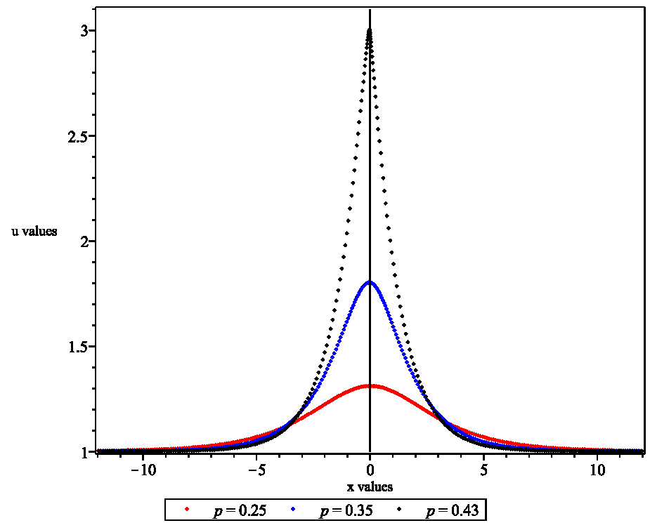
(a) Smooth soliton solutions

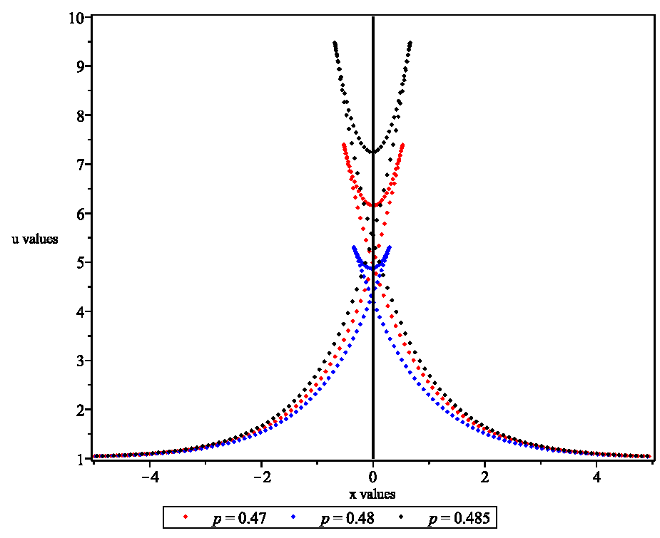
(b) Symmetric singular soliton solutions

Fig. 1: Two different kinds of solutions for the semi-discrete mCH equation at $t=0$. (a) Smooth soliton solutions, (b) Symmetric singular soliton solutions.

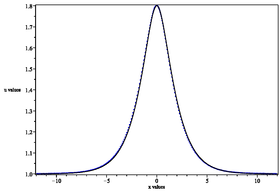
(a) Smooth soliton solutions

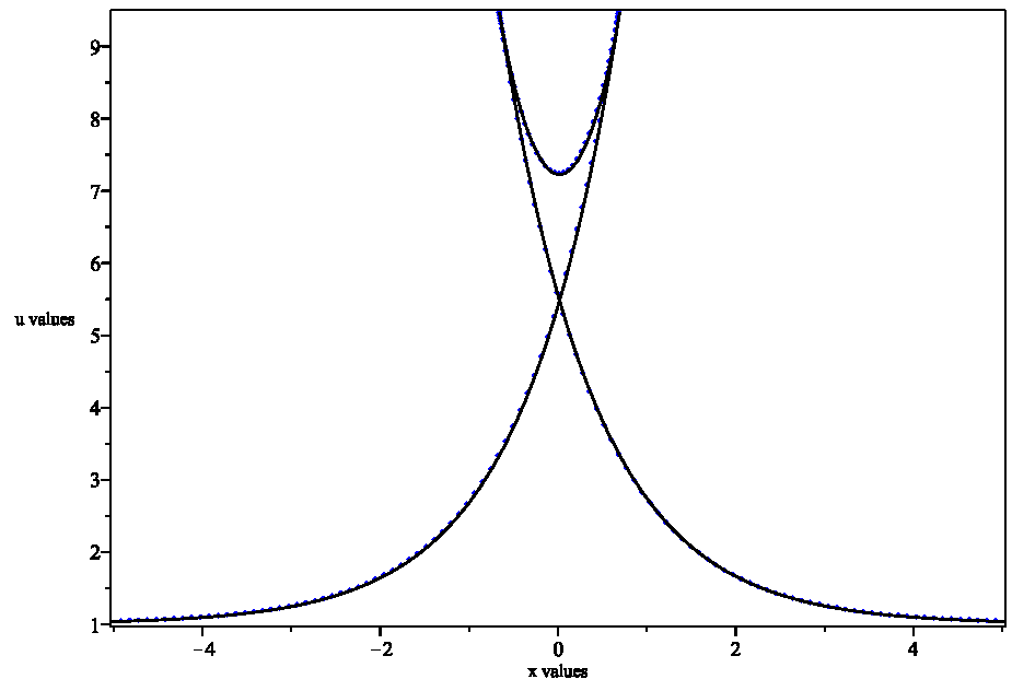
(b) Symmetric singular soliton solutions

Fig. 2: Comparison between the one-soliton solution for the mCH equation and the semi-discrete mCH equation at $t=0$; solid line: mCH equation, dot: semi-discrete mCH equation. (a) $p=0.35$, (b) $p=0.485$.

3.3.2 Two-soliton solutions

The $\tau$-functions for the two-soliton solution of the semi-discrete mCH equation in Theorem 3.2 are

$$f_{k}\propto 1+z_{1}^{-k}e^{\zeta_{1}}+z_{2}^{-k}e^{\zeta_{2}}+\left(\frac{p_{1}-p_{2}}{p_{1}+p_{2}}\right)^{2}(z_{1}z_{2})^{-k}e^{\zeta_{1}+\zeta_{2}},$$ (67)

$$g_{k}\propto 1+\frac{1-2p_{1}}{1+2p_{1}}z_{1}^{-k}e^{\zeta_{1}}+\frac{1-2p_{2}}{1+2p_{2}}z_{2}^{-k}e^{\zeta_{2}}+\frac{1-2p_{1}}{1+2p_{1}}\frac{1-2p_{2}}{1+2p_{2}}\left(\frac{p_{1}-p_{2}}{p_{1}+p_{2}}\right)^{2}(z_{1}z_{2})^{-k}e^{\zeta_{1}+\zeta_{2}},$$ (68)

with $z_{i}=\frac{1-bp_{i}}{1+bp_{i}}$ and $\zeta_{i}=-\frac{4p_{i}}{1-4p_{i}^{2}}\tau+\zeta_{i0}$. We take $b=0.1$ and $\zeta_{i0}=0$. Fig. 3 displays the collision between two smooth solitons. One can see that the soliton with a higher peak moves faster than the lower one. It can be found that there is a strong agreement between the two-soliton solution of the semi-discrete mCH equation and the mCH equation.

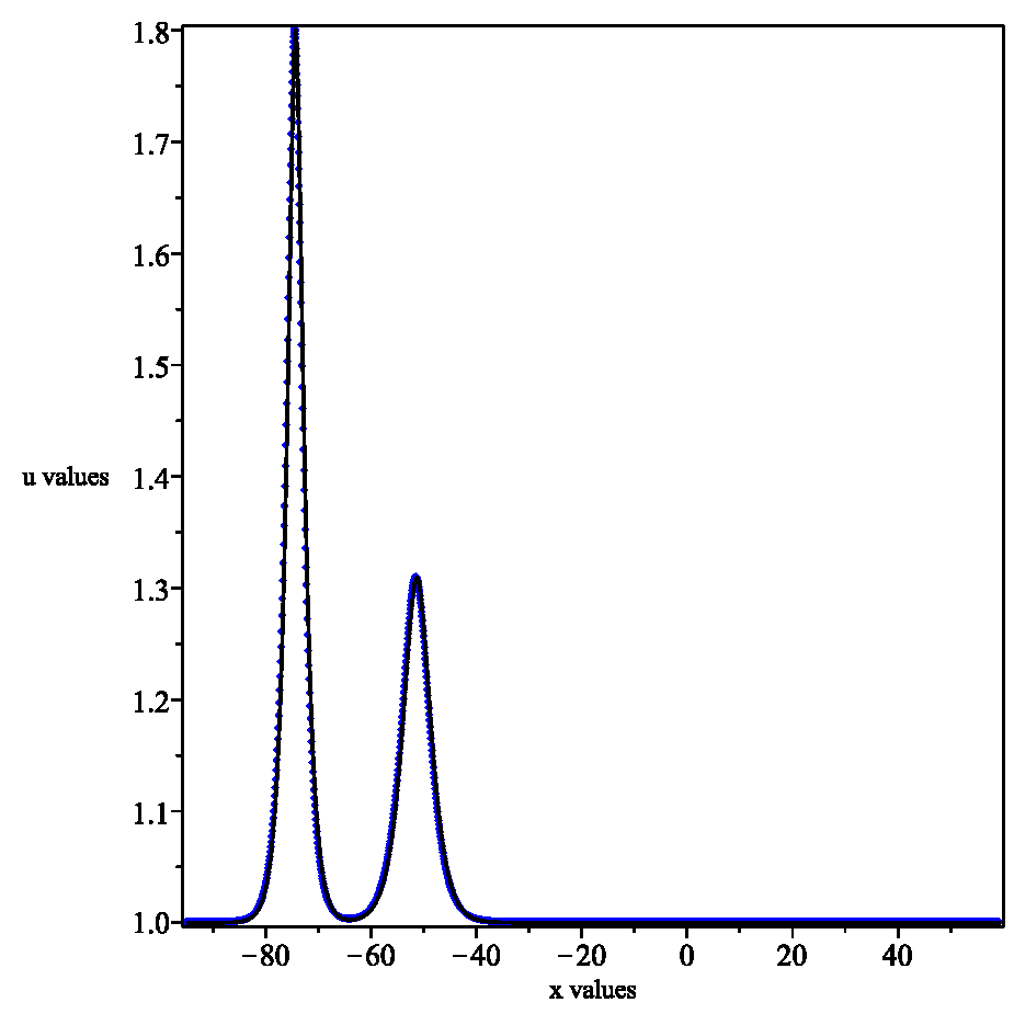
(a) $t=-15$

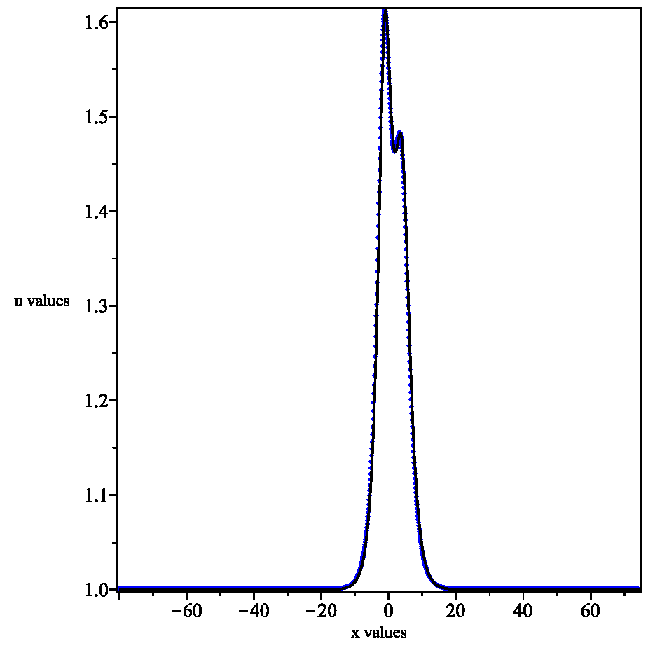
(b) $t=0$

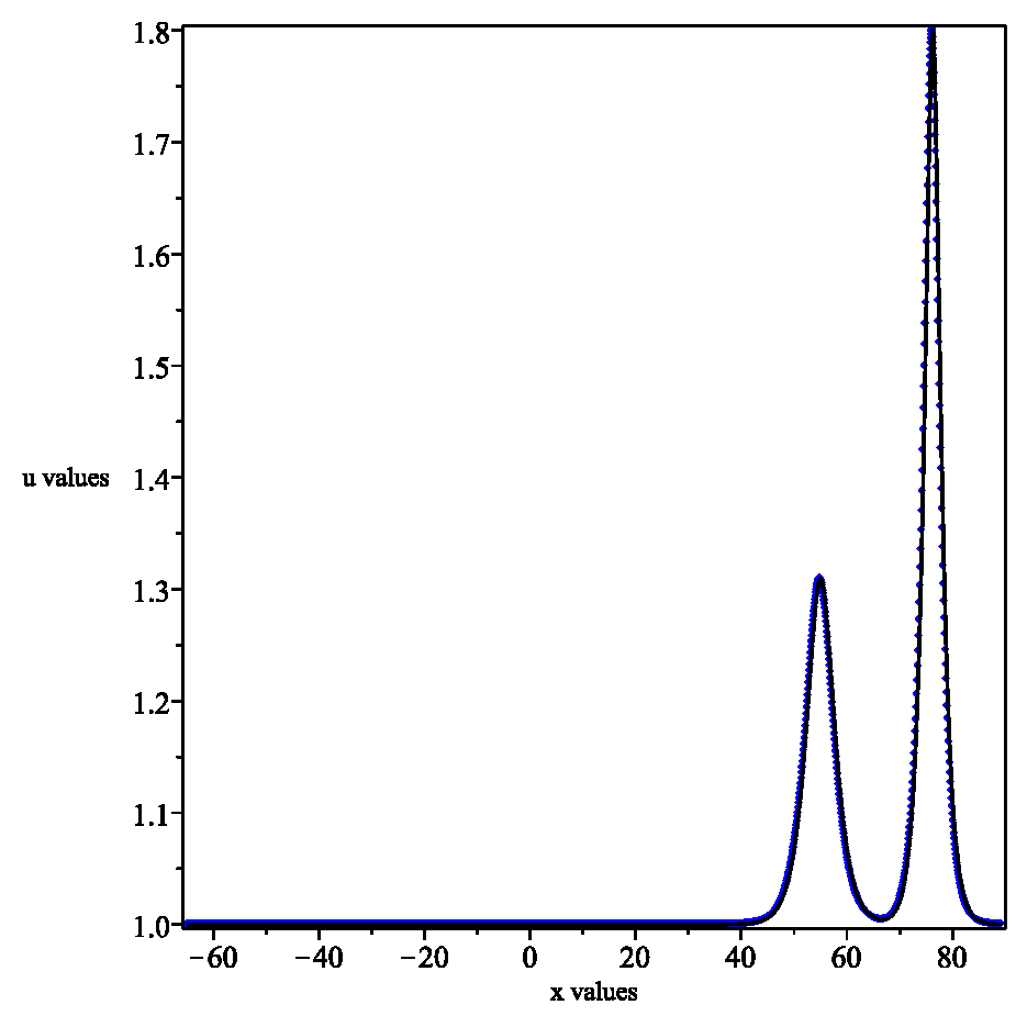
(c) $t=15$

Fig. 3: Comparison between the two-soliton solution of the mCH and the semi-discrete mCH equation with $p_{1}=0.25$, $p_{2}=0.35$; solid line: mCH equation; dot: semi-discrete mCH equation. (a)$t=-15$, (b)$t=0$, (c)$t=15$.

4 Conclusion

In this paper, starting from the discrete KP equation, we have constructed an integrable semi-discrete analog of the mCH equation with cubic nonlinearity through Miwa transformation and a series of reductions. Gram-type determinant solutions for the semi-discrete mCH equation has been derived. Smooth soliton solutions and symmetric singular soliton solutions are generated from the determinant formulas. The discrete KP equation is once again shown to be the fundamental equation for integrable systems, in line with the findings by Hirota, Ohta, Tsujimoto, Nimmo, and so on. Furthermore, there are a few aspects that deserve further study. Firstly, the Lax pair associated with the semi-discrete mCH equation is still unknown. How to generate the Lax pair for the derived discrete integrable systems based on the Lax pair of discrete KP equation is left to be investigated. Secondly, here we only find semi-discrete version of the mCH equation and the full-discrete analogue of the mCH is left to be considered. Thirdly, connections between the discrete KP equation and the two-component CH equation [48], the two-component mCH equation [49], the complex short pulse equation [50] and the massive Thirring model equation [51] are worth investigating.

References

- [1] Fuchssteiner B, Fokas AS. Symplectic structures, their Bäcklund transformations and hereditary symmetries. Physica D. 1981;4:47–66.
- [2] Fokas AS. On a class of physically important integrable equations. Physica D. 1995;87:145–150.
- [3] Fuchssteiner B. Some tricks from the symmetry-toolbox for nonlinear equations: generalizations of the Camassa-Holm equation. Physica D. 1996;95:229–243.
- [4] Olver PJ, Rosenau P. Tri-Hamiltonian duality between solitons and solitary-wave solutions having compact support. Phy Rev E. 1996;53:1900–1906.
- [5] Qiao Z. A new integrable equation with cuspons and W/M-shape-peaks solitons. J Math Phys. 2006 ;47:112701.
- [6] Qiao Z, Li XQ. An integrable equation with nonsmooth solitons. Theor Math Phys. 2011;167:214–221.
- [7] Fu Y, Gui G, Liu Y, Qu C. On the Cauchy problem for the integrable modified Camassa-Holm equation with cubic nonlinearity. J Differential Equations. 2013;255:1905–1938.
- [8] A. Alexandrou H, Mantzavinos D. The Cauchy problem for the Fokas-Olver-Rosenau-Qiao equation. Nonlinear Anal. 2014;95:499–529.
- [9] Luo Z, Qiao Z, Yin Z. On the Cauchy problem for a modified Camassa-Holm equation. Monatsh Math. 2020;193:857–877.
- [10] Boutet de Monvel A, Karpenko I, Shepelsky D. A Riemann-Hilbert approach to the modified Camassa-Holm equation with nonzero boundary conditions. J Math Phys. 2020;61:031504.
- [11] Xu J, Fan E. Long-time asyptotics behavior for the integrable modified Camassa-Holm equation with cubic nonlinearity. 2019;arXiv:1911.12554.
- [12] Yang Y, Fan E. On the long-time asymptotics of the modified Camassa-Holm equation in space-time solitonic regions. Adv Math. 2022;402:108340.
- [13] Kang, J, Liu, X, Olver, PJ, Qu, C. Liouville correspondence between the modified KdV hierarchy and its dual integrable hierarchy. J Nonlinear Sci. 2016;26:141–170.
- [14] Qu C, Fu Y, Liu Y. Well-posedness, wave breaking and peakons for a modified -Camassa-Holm equation. J Funct Anal. 2014;266:433–477.
- [15] Tang H, Liu Z. Well-posedness of the modified Camassa-Holm equation in Besov spaces. Z Angew Math Phys. 2015;66:1559–1580.
- [16] Gao Y, Li L, Liu JG. A dispersive regularization for the modified Camassa-Holm equation. SIAM J Math Anal. 2018;50:2807–2838.
- [17] Matsuno Y. Bäcklund transformation and smooth multisoliton solutions for a modified Camassa-Holm equation with cubic nonlinearity. J Math Phys. 2013;54:051504.
- [18] Hu H, Yin W, Wu H. Bilinear equations and new multi-soliton solution for the modified Camassa-Holm equation. Appl Math Lett. 2016;59:18–23.
- [19] Xia B, Zhou R, Qiao Z. Darboux transformation and multi-soliton solutions of the Camassa-Holm equation and modified Camassa-Holm equation. J Math Phys. 2016;57:103502.
- [20] Hou Y, Fan E, Qiao Z. The algebro-geometric solutions for the Fokas-Olver-Rosena-Qiao (FORQ) hierarchy. J Geo Phys. 2017;117:105–133.
- [21] Wang G, Liu QP, Mao H. Bäcklund transformation and nonlinear superposition formula. J Phys A. 2020;53:294003.
- [22] Bies PM, Górka P, Reyes, Enrique G. The dual modified Korteweg-de Vries-Fokas-Qiao equation: geometry and local analysis. J Math Phys. 2012;53:073710.
- [23] Gui G, Liu Y, Olver PJ, Qu C. Wave-breaking and peakons for a modified Camassa-Holm equation. Commun Math Phys. 2013;319:731–759.
- [24] Chang XK, Szmigielski J. Lax integrability of the modified Camassa-Holm equation and the concept of peakons. J Nonlinear Math Phys. 2016;23:563–572.
- [25] Chang XK, Szmigielski J. Liouville integrability of conservative peakons for a modified CH equation. J Nonlinear Math Phys. 2017;24:584–595.
- [26] Chang XK, Szmigielski J. Lax integrability and the peakon problem for the modified Camassa-Holm equation. Comm Math Phys. 2018;358:295–341.
- [27] Gao Y, Li L, Liu, JG. Patched peakon weak solutions of the modified Camassa-Holm equation. Physica D. 2019;390:15–35.
- [28] Gao Y. On conservative sticky peakons to the modified Camassa-Holm equation. J Differential Equations. 2023;365:486–520.
- [29] Liu Y, Olver PJ, Qu C, Zhang S. On the blow-up of solutions to the integrable modified Camassa-Holm equation. Anal Appl (Singap). 2014;12:355–368.
- [30] Chen RM, Liu Y, Qu C, Zhang S. Oscillation-induced blow-up to the modified Camassa-Holm equation with linear dispersion. Adv Math. 2015;272:225–251.
- [31] Li J, Liu Y. Stability of Solitary Waves for the Modified Camassa-Holm Equation. Ann PDE. 2021;7:14.
- [32] Liu X, Liu Y, Qu C. Orbital stability of the train of peakons for an integrable modified Camassa-Holm equation. Adv Math. 2014;255:1–37.
- [33] Hietarinta J, Joshi N, Nijhoff FW Discrete Systems and Integrability, (Cambridge University Press, 2016).
- [34] Fu, Wei; Nijhoff, Frank W. On reductions of the discrete Kadomtsev-Petviashvili-type equations. J. Phys. A 2017;50:505203.
- [35] Feng BF, Maruno K, Ohta Y. Integrable discretizations of the short pulse equation. J Phys A. 2010;43:085203.
- [36] Feng BF, Maruno K, Ohta Y. Integrable semi-discretization of a multi-component short pulse equation. J Math Phys. 2015;56:043502.
- [37] Yu GF, Xu ZW. Dynamics of a differential-difference integrable (2+1)-dimensional system. Phys Rev E. 2015;91:062902.
- [38] Ohta Y, Maruno K, Feng BF. An integrable semi-discretization of the Camassa-Holm equation and its determinant solution. J Phys A: Math Theor. 2008;41:355205.
- [39] Feng BF, Maruno K, Ohta Y. Integrable discretizations for the short-wave model of the Camassa-Holm equation. J Phys A: Math Theor. 2010;43:265202.
- [40] Feng BF, Maruno K, Ohta Y. Integrable semi-discrete Degasperis-Procesi equation. Nonlinearity. 2017;30:2246–2267.
- [41] Feng BF, Sheng HH, Yu GF. Integrable semi-discretizations and self-adaptive moving mesh method for a generalized sine-Gordon equation. Numer Algorithms. 2023;94:351–370.
- [42] Sheng HH, Feng BF, Yu GF. Integrable discretizations for a generalized sine-Gordon equation and the reductions to the sine-Gordon equation and the short pulse equation. J. Nonlinear Sci.. 2024; 34–55. https://doi.org/10.1007/s00332-024-10030-w.
- [43] Sheng HH, Yu GF, Feng BF. An integrable semidiscretization of the modified Camassa-Holm equation with linear dispersion term. Stud Appl Math. 2022;149:230–265.
- [44] Matsuno Y. Smooth and singular multisoliton solutions of a modified Camassa-Holm equation with cubic nonlinearity and linear dispersion. J Phys A. 2014;47:125203.
- [45] Hirota R. Discrete analogue of a generalized Toda equation. J Phys Soc Japan. 1981;50:3785–3791.
- [46] Miwa T. On Hirota’s difference equations. Proc Japan Acad Ser A Math Sci. 1982;58:9–12.
- [47] Ohta Y, Hirota R, Tsujimoto S, Imai T. Casorati and discrete Gram type determinant representations of solutions to the discrete KP hierarchy. J Phys Soc Jpn. 1993;62:1872–1886.
- [48] Chen M, Liu S, Zhang Y. A two-component generalization of the Camassa-Holm equation and its solutions. Lett Math Phys. 2006;75:1–15.
- [49] Song J, Qu C, Qiao Z. A new integrable two-component system with cubic nonlinearity. J Math Phys. 2011;52:013503.
- [50] Feng BF. Complex short pulse and coupled complex short pulse equations. Physica D. 2015;297:62–75.
- [51] Thirring WE. A Soluble Relativistic Field Theory. Ann Phys. 1958;3:91.
- [52] Mikhailov AV. Integrability of the two-dimensional Thirring model. JETP Lett. 1976;23:320–323.