Out-of-distribution generalization under random, dense distributional shifts

Abstract

Many existing approaches for estimating parameters in settings with distributional shifts operate under an invariance assumption. For example, under covariate shift, it is assumed that $p(y|x)$ remains invariant. We refer to such distribution shifts as sparse, since they may be substantial but affect only a part of the data generating system. In contrast, in various real-world settings, shifts might be dense. More specifically, these dense distributional shifts may arise through numerous small and random changes in the population and environment. First, we will discuss empirical evidence for such random dense distributional shifts and explain why commonly used models for distribution shifts—including adversarial approaches—may not be appropriate under these conditions. Then, we will develop tools to infer parameters and make predictions for partially observed, shifted distributions. Finally, we will apply the framework to several real-world data sets and discuss diagnostics to evaluate the fit of the distributional uncertainty model.

1 Introduction

Distribution shift is a persistent challenge in statistics and machine learning. For example, we might be interested in understanding the determinants of positive outcomes in early childhood education. However, the relationships among learning outcomes and other variables can shift over time and across locations. This makes it challenging to gain actionable knowledge that can be used in different situations. As a result, there has been a surge of interest in robust and generalizable machine learning. Existing approaches can be classified as invariance-based approaches and adversarial approaches.

Invariance-based methods assume that the shifts are “sparse” in a sense that they only affect a sub-space of the data distribution [Pan and Yang, 2010, Baktashmotlagh et al., 2013]. For example, under covariate shift [Quinonero-Candela et al., 2009], the distribution of the covariates changes while the conditional distribution of the outcomes given the covariates stays invariant. In causal representation learning [Schölkopf et al., 2021], the goal is to disentangle the distribution into independent causal factors; based on the assumption that spurious associations can be separated from invariant associations. Both approaches assume that the shift affects only a sub-space of the data. We will call such shifts sparse distribution shifts.

Adversarial methods in robust machine learning consider “worst-case” perturbations. The idea is that some adversary can perturb the data either at the training [Huber, 1981] or deployment stage [Szegedy et al., 2014, Duchi and Namkoong, 2021]; and the goal is to learn a model that is robust to such deviations. While developing robust procedures is a worthwhile goal, worst-case perturbations might be too conservative in many real-world applications.

In this paper, we consider distributional shifts due to “random” and “dense” perturbations. As an example, consider replication studies. In replication studies, different research teams try to replicate results by following the same research protocol. Therefore, any distribution shift between the data may arise from the superposition of many unintended, subtle errors that affect every part of the distribution, which might be modeled as random. We call such shifts dense distributional shifts.

The random, dense distributional shift model has recently been used to quantify distributional uncertainty in parameter estimation problems [Jeong and Rothenhäusler, 2023] and has shown success in modelling real-world temporal shifts in refugee placement and unknown cluster structure in a randomized experiment [Bansak et al., 2024, Rothenhäusler and Bühlmann, 2023].

We will develop tools to measure the similarity between randomly perturbed distributions, infer parameters and predict outcomes for partially observed and shifted distributions. Perhaps surprisingly, these tools have a close relationship to synthetic controls [Abadie and Gardeazabal, 2003], which are a popular procedure for distribution generalization in panel data. One strength of our approach is that it applies to all data modalities, including discrete, ordinal, continuous and infinite-dimensional data, and that it can be used in conjunction with modern machine learning tools based on empirical risk minimization.

In addition, it will turn out that much of the language that we use to describe how random variables relate to each other (covariance, regression,…) can directly be used to describe how randomly shifted distributions relate to each other. Broadly speaking, our framework provides a new language for dense distributional shifts and brings clarity regarding how we should infer parameters, predict outcomes, and quantify uncertainty under dense distributional shifts.

1.1 Related work

This work addresses domain adaptation problems under a specific class of random distributional shifts. Domain adaptation methods generally fall into two main categories [Pan and Yang, 2010]. The first type involves re-weighing, where training samples are assigned weights that take the distributional change into account [Long et al., 2014, Li et al., 2016]. For example, under covariate shift, training samples can be re-weighted via importance sampling [Gretton et al., 2009, Shimodaira, 2000, Sugiyama et al., 2008]. Another type aims to learn invariant representations of features [Argyriou et al., 2007, Baktashmotlagh et al., 2013]. If representations are invariant between the training and target distributions, utilizing these representations into prediction algorithm could improve generalizability. Under dense distributional shifts, as we will see in Section 2, instance-specific weights can lead to unstable estimators or even be undefined due to overlap violations. Furthermore, under dense distributional shifts there might be no invariant representation. Thus, from a classical domain adaptation perspective, dense distribution shifts are a challenging setting. Under random distribution shift (which may include random overlap violations), we will introduce a distributional CLT. This will allow for statistical inference, in a setting that seems challenging from the perspective of existing models.

The proposed method shares methodological similarities with synthetic controls [Abadie and Gardeazabal, 2003], as both approaches search for a linear combination of donor distributions (corresponding to untreated units in synthetic controls) to represent a target distribution (corresponding to the treated units in synthetic controls). Synthetic controls are applied to panel data and often assume a linear factor model for a continuous outcome of interest [Doudchenko and Imbens, 2016, Abadie et al., 2007, Bai, 2009, Xu, 2017, Athey et al., 2021]. Our framework can be seen as a justification for synthetic control methods under random distributional shifts. In addition, our procedure can be applied to model distribution shifts with or without time structure for any type of data (discrete, continuous, ordinal). Furthermore, our framework allows for straightforward generalizations to empirical risk minimization, which includes many modern machine learning tools.

Our procedure is also loosely related to meta-analysis. Meta-analysis is a statistical procedure for combining data from multiple studies [Higgins et al., 2009]. Traditional meta-analysis relies on the assumption that the effect size estimates from different studies are independent. However, in real-world applications, this independence assumption often does not hold true. There are different strategies to handle dependencies. These include averaging the dependent effect sizes within studies into a single effect [Wood, 2008], incorporating dependencies into models through robust variance estimation [Hedges et al., 2010], or through multilevel meta-analysis where they assume a cluster structure and model dependence within and between clusters [Cheung, 2014]. In meta-regression, the effect sizes are expressed as linear functions of study characteristics, and they are independent conditional on these study characteristics [Borenstein et al., 2009, Hartung et al., 2008]. Bayesian hierarchical models with prior on model parameters can also be used to model dependency [Higgins et al., 2009, Lunn et al., 2013]. Compared to these procedures, our approach allows for correlations between studies and can be applied even when there is no hierarchical structure and no summary study characteristics are available. While Bayesian hierarchical models often pose computational challenges and sensitivity to prior distributions, our method is computationally efficient and does not require making decisions about prior distributions. Additionally, our procedure can be used in conjunction with generic machine learning tools based on empirical risk minimization.

The classical robust statistics literature [Huber, 1981] addresses distributional perturbations by investigating the worst-case behavior of a statistical functional over a fixed neighborhood of the model. More recently, distributional uncertainty sets based on $f$-divergence have been linked to distributionally robust optimization [Ben-Tal et al., 2013, Duchi et al., 2021]. As we will see in Section 2, such bounds can be overly conservative under dense distributional shifts. The upshot is that while random shifts might appear large in Kullback-Leibler divergence or total variation distance, some of the random shifts cancel out under a distributional CLT.

In this paper, we model multiple correlated distributions using random distributional perturbation model introduced in Jeong and Rothenhäusler [2023], where dense distributional shifts emerge as the superposition of numerous small random changes. In Jeong and Rothenhäusler [2023], a single perturbed distribution is considered. In our paper, we extend this model to address multiple perturbed distributions that are possibly correlated.

1.2 Outline of the Paper

In Section 2, we present empirical evidence of multiple correlated dense distributional shifts and introduce the random distributional perturbation model. In Section 2.1, we then discuss why, from a classical domain adaptation perspective, dense distributional shifts are a challenging setting. In Section 3, we establish the foundations for domain adaptation under dense distributional shifts. In Section 3.3, we generalize our method to empirical risk minimization, such that it can be used in conjunction with modern machine learning tools. In Section 4 and Section 5, we apply our framework to several real-world data sets and demonstrate the robustness of our method. We conclude in Section 6.

2 Distributional Uncertainty

Due to a superposition of many random, small changes, a data scientist might not draw samples from the target distribution $\mathbb{P}^{0}$ but from several randomly perturbed distributions $\mathbb{P}^{1},\dots,\mathbb{P}^{K}$. More specifically, we assume that a data scientist has $K$ datasets, with the $k$-th dataset being an independent sample from a perturbed distribution $\mathbb{P}^{k}$. Intuitively speaking, some of these distributions might be similar to each other, while others might be very different. For instance, one replication study might closely resemble another due to collaboration among investigators. Additionally, a data set obtained from California might be more similar to one from Washington than to one from Wyoming.

We illustrate the scenario where multiple data sets exhibit distributional correlations using the GTEx data. The GTEx V6 data offers pre-processed RNA-seq gene-expression levels collected from 450 donors across 44 tissues. Treating each tissue as an individual study, we have 44 different data sets. Each data set from tissue $k$ is considered as an independent sample from a perturbed distribution $\mathbb{P}^{k}$, where $\mathbb{P}^{\bullet}$ represents a joint distribution of all gene-expression levels. Some of these data sets are likely to be correlated due to factors such as an overlap of donors and the proximity between tissues. Empirical evidence of this correlation is presented in the left side of Figure 1, where each row and column corresponds to a tissue, and each dot represents a standardized covariance between gene expression levels of a randomly selected gene-pair, among the observations in the tissue. We randomly sample 1000 gene-pairs. We can see that some tissues exhibit a clear linear relationship. In the following, we will introduce a distribution shift model that implies this linear relationship.

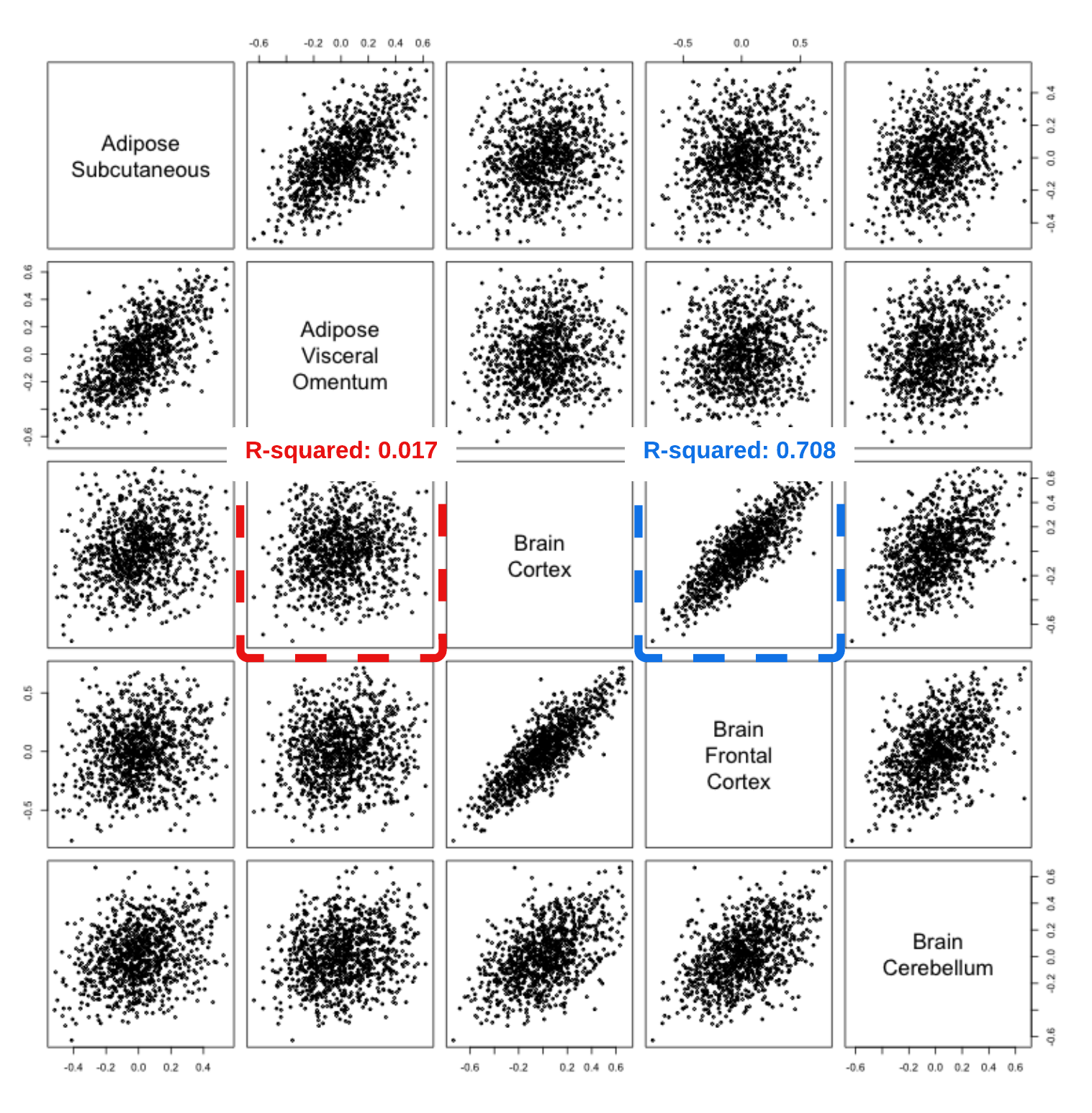
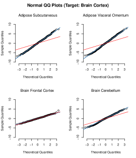
Figure 1: (Left) Linear relationships between tissues: Each row and column corresponds to one tissue, with each dot representing the standardized covariance of the gene expression levels of a randomly selected gene pair. Note that certain tissues exhibit a linear relationship. For instance, a notable linear relationship is observed within the blue squared box, where a simple linear regression yielded an R-squared value of 0.708. In contrast, in the red squared box, a linear relationship is not evident, as indicated by the simple linear regression result with an R-squared value of 0.017. (Right) QQ plots of (2) for various test functions for different perturbed tissues when the target tissue is brain cortex. The red line represents the expected QQ line if the perturbed data were all drawn i.i.d. from the target distribution (brain cortex).

To model the relatedness of multiple data sets, we will assume that each $\mathbb{P}^{k}$ is a random perturbation of a common target distribution $\mathbb{P}^{0}$. Then, we adopt the random distributional perturbation model in Jeong and Rothenhäusler [2023], where dense distributional shifts emerge as the superposition of numerous small random changes, to construct perturbed distributions $\mathbb{P}^{1},\dots,\mathbb{P}^{K}$. In this random perturbation model, probabilities of events from a random probability measure $\mathbb{P}^{k}$ are slightly up-weighted or down-weighted compared to the target distribution $\mathbb{P}^{0}$.

Without loss of generality, we construct distributional perturbations for uniform distributions on $[0,1]$. A result from probability theory shows that any random variable $D$ on a finite or countably infinite dimensional probability space can be written as a measurable function $D\stackrel{{\scriptstyle d}}{{=}}h(U)$, where $U$ is a uniform random variable on $[0,1]$. With the transformation $h$, the construction of distributional perturbations for uniform variables can be generalized to the general cases by using

$$\mathbb{P}^{k}(D\in\bullet)=\mathbb{P}^{k}(h(U)\in\bullet).$$

Let us now construct the perturbed distribution $\mathbb{P}^{k}$ for a uniform variable. Take $m$ bins $I_{j}=[(j-1)/m,j/m]$ for $j=1,\dots,m$. Let $W^{k}_{1},\dots,W^{k}_{m}$ be i.i.d. positive random variables with finite variance. We define the randomly perturbed distribution $\mathbb{P}^{k}$ by setting

$$\mathbb{P}^{k}(U\in\bullet)=\sum_{j}\mathbb{P}^{0}(U\in I_{j}\cap\bullet)\cdot\frac{W^{k}_{j}}{\sum_{j=1}^{m}W^{k}_{j}/m}.$$

Conditionally on $W=(W_{j}^{k})_{k=1,\ldots,K;j=1,\ldots,m}$, let $\mathcal{D}_{k}=\{D_{k1},\ldots,D_{kn_{k}}\}$ be i.i.d. $n_{k}$ draws from $\mathbb{P}^{k}$ for each $k=1,\dots,K$. Let $m=m(n)$ such that $\frac{m(n)}{\min(n_{1},\dots,n_{K})}$ converges to 0. This is the regime where the distributional uncertainty is of higher order than the sampling uncertainty.

Notation

Let $\mathbb{P}^{0}$ be the target distribution on $\mathcal{D}$, and $\mathbb{P}^{k}$ be the perturbed distribution on $\mathcal{D}$ conditioned on $(W_{j}^{k})_{j=1}^{m}$. We draw an i.i.d. sample $\mathcal{D}_{k}=\{D_{ki}\}_{i=1}^{n_{k}}$ from $\mathbb{P}^{k}$, conditioned on $(W_{j}^{k})_{j=1}^{m}$. Let $P$ be the marginal distribution of $\{\{D_{ki}\}_{i=1}^{n_{k}},\{W_{j}^{k}\}_{j=1}^{m}\}_{k=1}^{K}$. We denote $E$ as the expectation under $P$, $\mathbb{E}^{0}$ as the expectation under $\mathbb{P}^{0}$, and $\mathbb{E}^{k}$ as the expectation under $\mathbb{P}^{k}$. Moreover, we denote $\hat{\mathbb{E}}^{k}$ as the sample average in $\mathcal{D}_{k}$. We write $\text{Var}_{P}$ for the variance under $P$ and $\text{Var}_{\mathbb{P}^{0}}$ for the variance under $\mathbb{P}^{0}$.

Theorem 1 (Distributional CLT).

Under the assumptions we mentioned above, for any Borel measurable square-integrable function $\phi_{k}:\mathcal{D}_{k}\xrightarrow[]{}\mathbb{R}$ for $k=1,\dots,K$, we have

$$\sqrt{m}\left(\begin{pmatrix}\hat{\mathbb{E}}^{1}[\phi_{1}(D)]\\ \vdots\\ \hat{\mathbb{E}}^{K}[\phi_{K}(D)]\end{pmatrix}-\begin{pmatrix}\mathbb{E}^{0}[\phi_{1}(D)]\\ \vdots\\ \mathbb{E}^{0}[\phi_{K}(D)]\end{pmatrix}\right)\xrightarrow[]{d}N\left(0,\Sigma^{W}\odot\text{Var}_{\mathbb{P}^{0}}(\phi(D))\right)$$ (1)

where $\phi(D)^{\intercal}=(\phi_{1}(D),\dots,\phi_{K}(D))\in\mathbb{R}^{K}$, and $\Sigma^{W}\in\mathbb{R}^{K\times K}$ has

$$(\Sigma^{W})_{ij}=\frac{Cov_{P}(W^{i},W^{j})}{E[W^{i}]E[W^{j}]}.$$

Here, $\odot$ denotes element-wise multiplication (Schur product).

Remark 1.

Consider $K+1$ perturbed distributions $\mathbb{P}^{1},\dots,\mathbb{P}^{K},\mathbb{P}^{K+1}$ generated from the common parent distribution $\mathbb{P}^{0}$ under the random perturbation model. If our target distribution is $\mathbb{P}^{K+1}$ instead of the parent distribution $\mathbb{P^{0}}$, we still have

$$\sqrt{m}\left(\begin{pmatrix}\hat{\mathbb{E}}^{1}[\phi_{1}(D)]\\ \vdots\\ \hat{\mathbb{E}}^{K}[\phi_{K}(D)]\end{pmatrix}-\begin{pmatrix}\mathbb{E}^{K+1}[\phi_{1}(D)]\\ \vdots\\ \mathbb{E}^{K+1}[\phi_{K}(D)]\end{pmatrix}\right)\xrightarrow[]{d}N\left(0,\Sigma^{W}\odot\text{Var}_{\mathbb{P}^{0}}(\phi(D))\right)$$

for a different distributional covariance matrix $\Sigma^{W}$. The details can be found in the Appendix A.4.

Remark 2.

The variance under the target distribution $\text{Var}_{\mathbb{P}^{0}}(\phi(D))$ can be estimated via the empirical variance of $\phi$ on the pooled data $\{(D_{ki})_{i=1}^{n_{k}}\}_{k=1}^{K}$. Then, if $\phi$ has a finite fourth moment, we have $\widehat{\text{Var}}_{\mathbb{P}^{0}}(\phi(D))=\text{Var}_{\mathbb{P}^{0}}(\phi(D))+o_{p}(1)$. The details can be found in the Appendix A.5.

An extended version of Theorem 1 where $\phi_{k}:\mathcal{D}_{k}\xrightarrow[]{}\mathbb{R}^{L}$ for some $L\geq 1$ and the proof of Theorem 1 can be found in the Appendix, Section A.

Theorem 1 tells us that $(\Sigma_{ij}^{W})/m$ is the asymptotic covariance of $\hat{\mathbb{E}}^{i}[\phi(D)]$ and $\hat{\mathbb{E}}^{j}[\phi(D)]$ for any Borel-measurable square-integrable function $\phi$ with unit variance under $\mathbb{P}^{0}$. Remarkably, under our random distributional perturbation model, a $(K+\binom{K}{2})$-dimensional parameter $\Sigma^{W}$ quantifies the similarity of multiple distributions and captures all possible correlations of all square-integrable functions.

Distributional covariance.

We call $\Sigma^{W}/m$ the covariance between distributional perturbations. Two perturbed distributions $\mathbb{P}^{k}$ and $\mathbb{P}^{k^{\prime}}$ are positively correlated if $\Sigma_{kk^{\prime}}^{W}>0$. This means that when one perturbation slightly increases the probability of a certain event $A$, the other distribution tends to slightly increase the probability of this event as well. This can be seen by choosing the test function $\phi_{k}=1_{D\in A}$:

$$\text{Cov}_{P}(\hat{\mathbb{P}}^{k}(D\in A),\hat{\mathbb{P}}^{k^{\prime}}(D\in A))=\text{Cov}_{P}(\hat{\mathbb{E}}^{k}[1_{D\in A}],\hat{\mathbb{E}}^{k^{\prime}}[1_{D\in A}])\approx\frac{\Sigma_{k,k^{\prime}}^{W}}{m}\text{Var}_{\mathbb{P}^{0}}(1_{D\in A}).$$

However, if two perturbed distributions are negatively correlated, a (random) increase in the probability of an event under one distribution would often coincide with a (random) decrease in the probability of this event under the other distribution, compared to $\mathbb{P}^{0}$.

The random shift model explains the linear patterns in the GTEx scatterplot.

Consider two perturbed distributions $\mathbb{P}^{1}$ and $\mathbb{P}^{2}$, and $L$ uncorrelated test functions with unit variances, $\phi_{1}(D),\dots,\phi_{L}(D)$. In the GTEx example, $\phi_{\ell}$ is a standardized product between gene expression levels of a randomly selected $\ell$-th gene pair. Moreover, in Appendix D, wee see that these $L$ test functions are approximately uncorrelated. From Theorem 1, we have

$$\sqrt{m}\left(\begin{pmatrix}\hat{\mathbb{E}}^{1}[\phi_{\ell}(D)]\\ \hat{\mathbb{E}}^{2}[\phi_{\ell}(D)]\end{pmatrix}-\begin{pmatrix}\mathbb{E}^{0}[\phi_{\ell}(D)]\\ \mathbb{E}^{0}[\phi_{\ell}(D)]\end{pmatrix}\right)\stackrel{{\scriptstyle d}}{{=}}\text{ }Z_{\ell}+o_{p}(1),$$

where

$$Z_{\ell}\stackrel{{\scriptstyle i.i.d}}{{\sim}}N\left(0,\begin{pmatrix}\Sigma_{11}^{W}&\Sigma_{12}^{W}\\ \Sigma_{21}^{W}&\Sigma_{22}^{W}\end{pmatrix}\right).$$

Therefore, $(\hat{\mathbb{E}}^{1}[\phi_{\ell}(D)]-\mathbb{E}^{0}[\phi_{\ell}(D)],\hat{\mathbb{E}}^{2}[\phi_{\ell}(D)]-\mathbb{E}^{0}[\phi_{\ell}(D)])$ for $\ell=1,\dots,L$, can be viewed as independent draws from a bivariate Gaussian distribution with distributional covariance $\Sigma^{W}/m$. This explains the linear patterns observed in the left plot of Figure 1. Gaussianity can be evaluated by QQ plots of the statistic:

$$\left(\frac{1}{n_{k}}+\frac{1}{n_{0}}\right)^{-1/2}\left(\frac{\frac{1}{n_{k}}\sum_{i=1}^{n_{k}}\phi_{\ell}(D_{ki})-\frac{1}{n_{0}}\sum_{i=1}^{n_{0}}\phi_{\ell}(D_{0i})}{\hat{\text{sd}}_{\mathbb{P}^{0}}(\phi_{\ell}(D))}\right).$$ (2)

The QQ-plots of the statistic in (2) are presented on the right-hand side of Figure 1, when the target tissue is set to be brain cortex. These plots indicate that statistics in (2) indeed follow a Gaussian distribution.

Special cases of the random perturbation model.

We present special cases of the random perturbation model to help develop some intuition about potential applications of the model.

Example 1 (Random shift across time).

Consider the case where $W_{j}^{k}=W_{j}^{k-1}+\epsilon_{k}$, where the $\epsilon_{k}$ have mean zero and are uncorrelated for $k=1,\ldots,K$. This can be used to model random distributional shifts across time. For example, at some time point, we might see (randomly) higher or lower percentage of old patients at a hospital. Similarly, one could also have an auto-regressive model $W_{j}^{k}=\frac{1}{2}W_{j}^{k-1}+\frac{1}{2}W_{j}^{k-2}+\epsilon_{k}$. Please note that these auto-regressive models are defined on the weights of the distribution and not the data itself. This allows us to model random distributional shift for different data modalities such as discrete, ordinal, or continuous sample spaces, with a single framework.

Example 2 (Independent shifts and meta analysis).

If the distributional perturbations $W_{j}^{k}$ are i.i.d. across $k=1,\ldots,K$, then $\Sigma^{W}$ is a diagonal matrix. Thus, for any $\phi\in L^{2}(\mathbb{P}^{0})$, $\hat{\theta}_{k}:=\frac{1}{n_{k}}\sum_{i=1}^{n_{k}}\phi(D_{ki})$ are asymptotically Gaussian and uncorrelated across $k=1,\ldots,K$. This implies a meta-analytic model

$$\hat{\theta}_{k}\stackrel{{\scriptstyle\text{i.i.d.}}}{{\approx}}N(\theta^{0},\tau^{2}),$$ (3)

where $\tau^{2}=\frac{\Sigma_{kk}^{W}}{m}\text{Var}_{\mathbb{P}^{0}}(\phi)$ and $\theta^{0}:=\mathbb{E}^{0}[\phi(D)]$. Thus, in this special case, the random perturbation model justifies a random effect meta-analysis.

Example 3 (Random shift between locations).

In general, the meta-analytic model might not hold since the distributional perturbations might not be independent or identically distributed across $k=1,\ldots,K$. As an example, data from California might be similar to data from Washington, but very different from data from Pennsylvania. In the synthetic control literature, it is popular to model data distributions from different locations as (approximate) mixtures of each other. For example, data from California might be well approximated by a mixture of Washington and Nevada. In our framework, this can be expressed as

$$W^{\text{California}}=.7\cdot W^{\text{Washington}}+.3\cdot W^{\text{Nevada}}+\epsilon,$$ (4)

where $\epsilon$ is mean-zero noise.

2.1 Why standard approaches fail under dense distributional shifts

Given that a real-world data set seems to exhibit patterns consistent with dense distributional shifts, we will discuss why standard domain adaptation approaches based on re-weighting or worst-case bounds may not be appropriate for dense distributional shifts.

First, one might try to re-weight the distribution $\mathbb{P}^{k}$ to resemble the target distribution $\mathbb{P}^{0}$. However, the Radon-Nikodym derivative

$$w(d)=\frac{\mathrm{d}\mathbb{P}^{0}}{\mathrm{d}\mathbb{P}^{k}}(d)$$ (5)

may be unbounded or undefined if $W_{j}^{k}=0$ for some $j$. In the causal inference community, this is known as the overlap problem. In our setting, statistical inference is still possible, even if $W_{j}^{k}$ can be arbitrarily small. The key point is that while overlap may be violated in the proposed model, it is violated in a random fashion.

Secondly, one could take an adversarial perspective to bound distributional errors. In this case, a statistician might be interested in

$$\min_{\mathrm{D}_{\mathrm{KL}}(\mathbb{P}^{\prime}|\mathbb{P}^{k})\leq\epsilon}\theta(\mathbb{P}^{\prime})\qquad\text{ or }\qquad\max_{\mathrm{D}_{\mathrm{KL}}(\mathbb{P}^{\prime}|\mathbb{P}^{k})\leq\epsilon}\theta(\mathbb{P}^{\prime}),$$

for some parameter of interest $\theta(\cdot)$ and the Kullback-Leibler divergence $\mathrm{D}_{\mathrm{KL}}(\cdot|\cdot)$. This approach requires knowledge of the strength of the shift $\mathrm{D}_{KL}(\mathbb{P}^{0}|\mathbb{P}^{k})$. Under the random distributional shift model, as $m\rightarrow\infty$,

$$\mathrm{D}_{\mathrm{KL}}(\mathbb{P}^{0}|\mathbb{P}^{k}) \stackrel{{\scriptstyle m\rightarrow\infty}}{{\rightarrow}}E[-\log(W^{k})]+\log(E[W^{k}]),$$

which can be large. However, even though the randomly perturbed distribution is far from the target distribution in terms of the KL divergence, the distributional errors cancel out to some extent due to the distributional CLT. This will allow us to derive bounds that are of order $1/\sqrt{m}$, instead of the constant order worst-case bound.

3 Distribution Generalization

In this section, we demonstrate how, under the random distributional perturbation model, we can share information across data sets from many different times and locations, and infer parameters of the partially observed target distribution.

We consider the following domain adaptation setting throughout the section; for the $k$-th source data ($k\in\{1,2,\dots,K\}$), we observe $n_{k}$ i.i.d. samples $\mathcal{D}_{k}=\{D_{k1},\dots,D_{kn_{k}}\}$ drawn from the donor distribution $\mathbb{P}^{k}$. Furthermore, there are $n_{0}$ i.i.d. samples from the target distribution $\mathbb{P}^{0}$, but we only observe a subset $X\subset D$ and have $\mathcal{D}_{0}=\{X_{01},\dots,X_{0n_{0}}\}$. The goal is to estimate $\mathbb{E}^{0}[\phi_{0}(D)]$ when direct estimation using $\hat{\mathbb{E}}^{0}[\phi_{0}(D)]$ is not feasible due to partial observation of the target data.

3.1 Optimal convex combinations of donor distributions

The target distribution $\mathbb{P}^{0}$ could be described by a convex combination of several donor distributions. For example, a replication study might be very similar to a combination of other replication studies since replication studies might be clustered in regions that have many universities. In our perturbation model, this means that the random weights $W^{k}_{j}$ might be correlated across $k=1,\ldots,K$. From a mathematical perspective, we would want to solve

$$\beta^{*}=\operatorname*{argmin}_{\beta:\beta^{\intercal}\mathbb{1}=1}E[(\mathbb{E}^{0}[\phi_{0}(D)]-\sum_{k}\beta_{k}\hat{\mathbb{E}}^{k}[\phi_{0}(D)])^{2}].$$

Here, the outer expectation is over both the randomness due to sampling and the distributional perturbation. We solve this equation with respect to the asymptotic distribution of $\mathbb{E}^{0}[\phi_{0}(D)]-\sum_{k}\beta_{k}\hat{\mathbb{E}}^{k}[\phi_{0}(D)]$. Using Theorem 1, this leads to the quadratic optimization problem

$$\beta^{*}=\operatorname*{argmin}_{\beta:\beta^{\intercal}\mathbb{1}=1}\beta^{\intercal}\Sigma^{W}\beta.$$ (6)

The interesting point is that $\beta^{*}$ does not depend on $\phi_{0}$. Therefore, we can use different test functions of $X$, $\phi_{\ell}(X)$, $\ell=1,\dots,L$ to estimate $\beta^{*}$. More specifically, we can estimate $\beta^{*}$ by solving

$$\hat{\beta}=\operatorname*{argmin}_{\beta:\beta^{\intercal}\mathbb{1}=1}\sum_{l=1}^{L}(\hat{\mathbb{E}}^{0}[\phi_{l}(X)]-\sum_{k}\beta_{k}\hat{\mathbb{E}}^{k}[\phi_{l}(X)])^{2}.$$ (7)

Then for the target function $\phi_{0}(D)$, we estimate $\mathbb{E}^{0}[\phi_{0}(D)]$ via

$$\sum_{k=1}^{K}\hat{\beta}_{k}\hat{\mathbb{E}}^{k}[\phi_{0}(D)].$$

Remark 3.

In practice, one might wonder how to choose different test functions $\phi_{l},l=1,\ldots,L$. From a theoretical standpoint, under the distributional uncertainty model, one can technically choose any function with finite variance. However, for actual applications, we suggest the following guideline. Our method considers a distribution $\mathbb{P}^{k}$ to be “close” to $\mathbb{P}^{0}$ if the averaged values of test functions on $\mathcal{D}_{k}$ closely align with the corresponding averaged values on $\mathcal{D}_{0}$. Therefore, these test functions $\phi$ should be chosen to capture the dimensions of the problem where a close match is important. For example, in the numerical experiments in Section 5, the target function of interest is the logarithmic value of income and using the means of covariates that are well-known to be related to the income variable as test functions demonstrates good performance. We also provide simple diagnostics, presented in Figure 2 as standard residual plots and normal QQ-plots, that allow one to assess the fit of the distributional perturbation model and the choice of test functions using multiple available data sets.

This is similar to synthetic control procedures [Abadie and Gardeazabal, 2003], where we search for a linear combination of donor distributions to represent a target distribution. Furthermore, there is an obvious connection to ordinary least-squares. In the following, we will make this connection more thorough. In particular, we will show that standard statistical results ($t$-test, $F$-test, confidence intervals) carry over to the distributional case. In Section 3.3, we will see how these ideas can be used in conjunction with modern machine-learning tools for empirical risk minimization.

3.2 Re-casting distributional regression as ordinary least-squares

In the following, we discuss how to form asymptotically valid confidence intervals for $\beta^{*}$ and perform inference. As discussed earlier, data scientists have $L$ different test functions $\phi_{1}(X),\dots,\phi_{L}(X)$. For now we assume that test functions are uncorrelated and have unit variances under $\mathbb{P}^{0}$. Later we will discuss cases where test functions are correlated and have different variances. In the previous section, we saw that $\hat{\beta}$ can be estimated via a least-squares problem with a linear constraint on the weights. To remove the linear constraint in equation (7), we perform the following reparametrization,

$$\hat{\beta}_{1:(K-1)} =\operatorname*{argmin}_{\beta}\sum_{l=1}^{L}\left((\hat{\mathbb{E}}^{0}[\phi_{l}(X)]-\hat{\mathbb{E}}^{K}[\phi_{l}(X)])-\sum_{k=1}^{K-1}\beta_{k}(\hat{\mathbb{E}}^{k}[\phi_{l}(X)]-\hat{\mathbb{E}}^{K}[\phi_{l}(X)])\right)^{2}.$$

We can obtain $\hat{\beta}_{K}$ via $\hat{\beta}_{K}=1-\sum_{k=1}^{K-1}\hat{\beta}_{k}$. We can re-write this as the following linear regression problem

$$\hat{\beta}_{1:(K-1)}=\operatorname*{argmin}_{\beta_{1:(K-1)}\in\mathbb{R}^{K-1}}\|\tilde{\Phi}^{0}-\tilde{\Phi}\beta_{1:(K-1)}\|_{2}^{2},$$

where the feature matrix in the linear regression is defined as

$$\tilde{\Phi}=\begin{pmatrix}\hat{\mathbb{E}}^{1}[\phi_{1}]-\hat{\mathbb{E}}^{K}[\phi_{1}]&\dots&\hat{\mathbb{E}}^{K-1}[\phi_{1}]-\hat{\mathbb{E}}^{K}[\phi_{1}]\\ \vdots&&\vdots\\ \hat{\mathbb{E}}^{1}[\phi_{L}]-\hat{\mathbb{E}}^{K}[\phi_{L}]&\dots&\hat{\mathbb{E}}^{K-1}[\phi_{L}]-\hat{\mathbb{E}}^{K}[\phi_{L}]\end{pmatrix}\in\mathbb{R}^{L\times(K-1)},$$

and the outcome vector in the linear regression is defined as

$$\tilde{\Phi}^{0}=\left(\hat{\mathbb{E}}^{0}[\phi_{1}]-\hat{\mathbb{E}}^{K}[\phi_{1}],\dots,\hat{\mathbb{E}}^{0}[\phi_{L}]-\hat{\mathbb{E}}^{K}[\phi_{L}]\right)^{\intercal}\in\mathbb{R}^{L\times 1}.$$

Since test functions were assumed to be uncorrelated and have unit variances under $\mathbb{P}_{0}$, using Theorem 1, rows of the feature matrix $\tilde{\Phi}$ and the outcome vector $\tilde{\Phi}^{0}$ are asymptotically i.i.d., with each row drawn from a centered Gaussian distribution. Therefore, the problem may be viewed as a standard multiple linear regression problem where the variance of the regression coefficient $\hat{\beta}_{1:(K-1)}$ is estimated as

$$\widehat{\text{Var}}(\hat{\beta}_{1:(K-1)})=(\tilde{\Phi}^{\intercal}\tilde{\Phi})^{-1}\hat{\sigma}^{2},$$

and the residual variance is calculated as

$$\hat{\sigma}^{2}=\frac{1}{L-K+1}\|\tilde{\Phi}^{0}-\tilde{\Phi}\hat{\beta}\|_{2}^{2}.$$

Different from standard linear regression, in our setting each column represents a data distribution and each row represents a test function, and Gaussianity does not hold exactly in finite samples. Therefore, a priori it is unclear whether standard statistical tests in linear regression (such as the $t$-test and the $F$-test) carry over to the distributional case. The following theorem tells us that the standard linear regression results still hold. Therefore, we can conduct statistical inference for the optimal weights $\beta^{*}$ in the same manner as we conduct t-tests and F-tests in a standard linear regression. The proof of Theorem 2 can be found in Appendix, Section B.

Theorem 2.

Assume that test functions $\phi_{1},\dots,\phi_{L}$ are uncorrelated and have unit variances under $\mathbb{P}^{0}$. Let $\tilde{\Phi}$ and $\hat{\sigma}^{2}$ be defined as above. Then, we have

$$\left((\tilde{\Phi}^{\intercal}\tilde{\Phi})^{-1}\hat{\sigma}^{2}\right)^{-\frac{1}{2}}\left(\hat{\beta}_{1:(K-1)}-\beta^{*}_{1:(K-1)}\right)\stackrel{{\scriptstyle d}}{{=}}t_{K-1}(L-K+1)+o_{p}(1),$$

where $t_{p}(d)$ stands for the $p$-dimensional multivariate t-distribution with $d$ degrees of freedom.

Remark 4 (Distributional t-test).

The data scientist wants to know whether the data set $\mathcal{D}_{i}$ should be included in the training set to explain the target distribution. Mathematically, this corresponds to testing the null hypothesis $\beta_{i}=0$. Thus, we consider the following hypotheses:

$$H_{0}:\beta_{i}=0,\quad H_{1}:\beta_{i}\neq 0.$$

The test statistic is defined as

$$t=\frac{\hat{\beta}_{i}}{\sqrt{\left(\left(\tilde{\Phi}^{\intercal}\tilde{\Phi}\right)^{-1}\hat{\sigma}^{2}\right)_{ii}}}.$$

From Theorem 2, under the null hypothesis,

$$t\sim t(L-K+1),$$

where $t(L-K+1)$ is a univariate $t$-distribution with $L-K+1$ degrees of freedom .

Remark 5 (Distributional F-test).

The data scientist wants to know whether each data set is equally informative for the target distribution or not. Mathematically, this corresponds to testing the null hypothesis $\beta_{i}=1/K$ for $i=1,\ldots,K$. Thus, we consider the following hypotheses:

$$H_{0}:\,\,\beta_{1}=\ldots=\beta_{K}=\frac{1}{K},$$

$$H_{1}:\,\,\beta_{i}\neq\frac{1}{K},\text{ for at least one }i.$$

The test statistic is defined as

$$F=\left(\hat{\beta}_{1:(K-1)}-\frac{1}{K}\cdot\bm{1}_{K-1}\right)^{\intercal}\left((\tilde{\Phi}^{\intercal}\tilde{\Phi})^{-1}\hat{\sigma}^{2}\right)^{-1}\left(\hat{\beta}_{1:(K-1)}-\frac{1}{K}\cdot\bm{1}_{K-1}\right)/(K-1).$$

From Theorem 2, under the null hypothesis,

$$F\sim F_{K-1,L-K+1},$$

where $F_{K-1,L-K+1}$ is a F-distribution with degrees of freedom $K-1$ and $L-K+1$.

Remark 6 (Distributional confidence intervals for parameters of the target distribution).

We will now discuss how to form asymptotically valid confidence intervals for $\mathbb{E}^{0}[\phi_{0}(D)]$ when $m\xrightarrow[]{}\infty$ and $L\xrightarrow[]{}\infty$. Here we assume that $\phi_{0}$ has a finite fourth moment under $\mathbb{P}^{0}$. Then, we can form $(1-\alpha)$-confidence intervals for $\mathbb{E}^{0}[\phi_{0}(D)]$ as follows

$$\sum_{k=1}^{K}\hat{\beta}_{k}\hat{\mathbb{E}}^{k}[\phi_{0}]\pm z_{1-\alpha/2}\cdot\sqrt{\widehat{\text{Var}}_{\mathbb{P}^{0}}(\phi_{0})}\cdot\sqrt{\frac{1}{L}\sum_{\ell=1}^{L}\left(\hat{\mathbb{E}}^{0}[\phi_{\ell}]-\sum_{k=1}^{K}\hat{\beta}_{k}\hat{\mathbb{E}}^{k}[\phi_{\ell}]\right)^{2}}.$$

Note that $\widehat{\text{Var}}_{\mathbb{P}^{0}}(\phi_{0})$ refers to the empirical variance of $\phi_{0}$ on the pooled donor data $(D_{ki})_{k=1,\ldots,K,i=1,\ldots,n_{k}}$. The proof of this result can be found in the Appendix, Section C.

Remark 7 (Distributional sample size and degrees of freedom).

Note that the asymptotic variance of “distributional” regression parameters $(\tilde{\Phi}^{\intercal}\tilde{\Phi})^{-1}\hat{\sigma}^{2}$ has the same algebraic form as the asymptotic variance for regression parameters in a standard Gaussian linear model. In the classical setting, the test statistics of regression parameters follow $t$-distributions with $n-p+1$ degrees of freedom, where $n$ is the sample size and $p$ is the number of covariates. In our setting, we have $L-K+1$ degrees of freedom, where $L$ corresponds to the number of test functions and $K$ corresponds to the number of donor distributions.

Remark 8 (Correlated test functions).

In the result above, we assumed that the $(\phi_{1}(X),\dots,\phi_{L}(X))$ are uncorrelated and have unit variances under $\mathbb{P}^{0}$. In practice, this might not be the case. In such cases, we can apply a linear transformation $T$ to the test functions in a pre-processing step to obtain uncorrelated test functions with unit variances. We define the transformation matrix $T=(\hat{\Sigma}^{\Phi})^{-1/2}$, where $\hat{\Sigma}^{\Phi}$ is an estimate of the covariance matrix $\Sigma^{\Phi}$ of $(\phi_{1}(X),\dots,\phi_{L}(X))$ on the pooled data. From Remark 2, if $(\phi_{1}(X),\dots,\phi_{L}(X))$ have finite fourth moments, we have $\hat{\Sigma}^{\Phi}=\Sigma^{\Phi}+o_{p}(1)$.

3.3 Empirical risk minimization under distributional uncertainty

In this section, we will sketch how one can use the previous results in conjunction with modern machine learning methods such as gradient boosting, random forests, or neural networks.

Let’s say we want to find $\theta^{0}=\arg\min\mathbb{E}^{0}[l(\theta,D)]$ for some loss function $l(\theta,D)$, but only observe the full data $D$ from the distributions $\mathbb{P}^{1},\ldots,\mathbb{P}^{K}$, but not for the target distribution $\mathbb{P}^{0}$. For any fixed weights $\beta_{1},\ldots,\beta_{K}$ with $\sum_{k=1}^{K}\beta_{k}=1$ and fixed $\theta$, Theorem 1 shows that

$$\sum_{k}\beta_{k}\hat{\mathbb{E}}^{k}[l(\theta,D)]$$ (8)

is asymptotically unbiased for $\mathbb{E}^{0}[l(\theta,D)]$, marginalized over both sampling uncertainty and distributional uncertainty. Thus, we want to choose the $\beta_{1},\ldots,\beta_{K}$ that minimize the variance. For any $\theta$, the variance of the criterion is minimized for the $\beta_{k}$ defined in equation (6). Using the plug-in estimator for $\hat{\beta}$ defined in equation (7), we can estimate $\theta^{0}$ via

$$\hat{\theta}=\operatorname*{argmin}\sum_{k}\hat{\beta}_{k}\hat{\mathbb{E}}^{k}[l(\theta,D)].$$ (9)

If some of the weights $\beta_{k}$ are negative, then weighted empirical risk minimization might not be well-defined (due to non-convexity of $\theta\mapsto\sum_{k}\hat{\beta}_{k}\hat{\mathbb{E}}^{k}[l(\theta,D)]$). This can be fixed by finding the best non-negative linear approximation of the target distribution, i.e. by setting

$$\hat{\beta}=\operatorname*{argmin}_{\beta:\beta^{\intercal}\mathbf{1}=1,\beta_{k}\geq 0}\sum_{l=1}^{L}\left(\hat{\mathbb{E}}^{0}[\phi_{l}(X)]-\sum_{k=1}^{K}\beta_{k}\hat{\mathbb{E}}^{k}[\phi_{l}(X)]\right)^{2}.$$ (10)

and then solving

$$\hat{\theta}=\operatorname*{argmin}\sum_{k}\hat{\beta}_{k}\hat{\mathbb{E}}^{k}[l(\theta,D)].$$ (11)

We will explore the performance of this approach in empirical examples.

4 GTEx Data

In this section, we illustrate our methods using the GTEx data. We will also run model diagnostics to evaluate model fit. The GTEx V6 data set provides RNA-seq gene-expression levels collected from 450 donors across 44 tissues.

Treating each tissue as a separate study, we have 44 different data sets. As shown in Figure 1, some tissues exhibit higher correlations than others. To demonstrate our method, we select 5 different tissues (same as in Figure 1): Adipose subcutaneous, Adipose visceral omentum, Brain cortex, Brain frontal cortex, and Brain cerebellum. Let brain cortex be our target tissue (the third tissue in Figure 1). The code and the data are available as R package dlm at https://github.com/yujinj/dlm.

For our test functions, we randomly sample 1000 gene-pairs and define a test function as the standardized product of gene-expression levels of a pair. In total, we have 1000 test functions. Most genes are known to be uncorrelated with each other, with the 90th percentile range of correlations between two different test functions being about $[-0.06,0.06]$. We employ group Lasso to estimate the sparse inverse covariance matrix. As the estimated inverse covariance matrix is close to a diagonal matrix (details provided in the Appendix D), we do not perform a whitening transformation.

The R package dlm (https://github.com/yujinj/dlm) contains a function dlm that performs distributional linear regressions:

    dlm(formula, test.function, data, whitening)

Here, the formula parameter specifies which model we want to fit. The test.function parameter represents considered test functions. The data parameter passes a list of data sets. The whitening parameter is a boolean indicating whether one wants to perform a whitening transformation. Additional details and descriptions of the function can be found on the GitHub page.

Below is the summary output of the dlm function with a model formula “Brain cortex $\sim$ Adipose subcutaneuous + Adipose visceral omentum + Brain frontal cortex + Brain cerebellum” with 1000 test functions defined as standardized products of randomly selected gene-pairs. Note that the summary output of the dlm function closely resembles that of the commonly used lm function.

Call:
dlm(formula = Brain_Cortex ~ Adipose_Subcutaneous + Adipose_Visceral_Omentum +
    Brain_Frontal_Cortex_BA9 + Brain_Cerebellum, test.function = phi,
    data = GTEx_data, whitening = FALSE)

Residuals:
     Min       1Q   Median       3Q      Max
-0.56838 -0.09436 -0.00604  0.08739  0.40917

Coefficients:
                           Estimate Std. Error t value Pr(>|t|)
Adipose_Subcutaneous     -0.0001295  0.0304036  -0.004   0.9966
Adipose_Visceral_Omentum  0.0462641  0.0250888   1.844   0.0655 .
Brain_Frontal_Cortex_BA9  0.7846112  0.0184325  42.567  < 2e-16 ***
Brain_Cerebellum          0.1692543  0.0217128   7.795 1.61e-14 ***
---
Signif. codes:  0 *** 0.001 ** 0.01 * 0.05 . 0.1   1

Residual standard error: 0.1377 on 997 degrees of freedom
Multiple R-squared:  0.5088,ΨAdjusted R-squared:  0.5073
F-statistic: 344.3 on 3 and 997 DF,  p-value: < 2.2e-16

The coefficient represents the estimated weight for each perturbed data set. Note that the sum of coefficients equals to one. The estimated weight for the brain-frontal-cortex data set is close to 1: 0.7846112. On the other hand, the estimated weights for adipose-subcutaneous and adipose-visceral-omentum data sets are close to 0: -0.0001295 and 0.0462641. This supports the observations made in Figure 1, where the brain-cortex data set (target) exhibits a higher correlation with the brain-frontal-cortex data set than others.

Let us discuss the summary output in more detail. All tests have in common that the probability statements are with respect to distributional uncertainty, that is, the uncertainty induced by the random distributional perturbations.

1. (Distributional t-test). The summary output provides a t-statistic and a p-value for each estimated weight. Based on the output, the estimated weight for the brain-frontal-cortex data set is highly significant (with a t-statistic 42.567 and a p-value less than $2\cdot 10^{-16}$). We have enough evidence to believe that the true optimal weight for the brain-frontal-cortex data set is nonzero, and thus we conclude that the brain-frontal-cortex data set is important for predicting the target data set. On the other hand, the estimated weights for the adipose-subcutaneous and adipose-visceral-omentum data sets are not statistically significant (with t-statistics -0.004 and 1.844 and p-values 0.9966 and 0.0655). We conclude those data sets are not as important as the brain-frontal-cortex data set for predicting the target data set.

2. (Distributional F-test). The summary output provides a F-statistic and a corresponding p-value for a null hypothesis: the optimal weights are uniform ($\beta^{*}=(0.25,0.25,0.25,0.25)$ in our example). This means that different data sets are equally informative in explaining the target data set. The F-statistic is given as 344.3, and under the null hypothesis, it follows the F-distribution with degrees of freedom 3 and 997. The resulting p-value is less than $2.2\cdot 10^{-16}$. Therefore, we reject the null hypothesis. From Figure 1 and the estimated weights, we can see that the brain-frontal-cortex and brain-cerebellum data sets are more informative in explaining the target data set than the adipose-subcutaneous and adipose-visceral-omentum data sets.

3. (R-squared). Usually, the coefficient of determination (R-squared) measures how much of the variation of a target variable is explained by other explanatory variables in a regression model. In our output, R-squared measures how much of the unexplained variance of a target dataset, compared to considering uniform weights, is explained by considering our proposed weights. Specifically, it is calculated as

   $$R^{2}=1-\frac{\text{RSS with estimated weights}}{\text{RSS with uniform weights}}.$$

   R-squared is close to 0 if the estimated weights are close to uniform weights.

Finally, we should consider diagnostic plots to evaluate the appropriateness of the fitted distribution shift model. This can be evaluated using a distributional Tukey-Anscombe and a distributional QQ-Plot. In contrast to conventional residual plots and QQ-Plots, each point in these plot corresponds to a mean of a test function instead of a single observation. Figure 2 shows that neither the QQ-Plot nor the TA plot indicate a deviation from the modelling assumptions.

Figure 2: The distributional residual plot and distributional QQ-Plot for the GTEx data. In contrast to conventional residual plots and QQ-Plots, each point corresponds to a mean of a test function instead of a single observation.

5 ACS Income Data

In this section, we demonstrate the effectiveness and robustness of our method when the training data set is obtained from multiple sources. We focus on the ACS Income data set [Ding et al., 2021] where the goal is to predict the logarithmic value of individual income based on tabular census data.

Similar as in Shen et al. [2023], we consider a scenario where we initially have a limited training data set from California (CA), and subsequently, we obtain additional training data set from Puerto Rico (PR). We iterate through the target state among the rest of 49 states. Note that there are substantial economic, job market, and cost-of-living disparities between CA and PR. Most of the states are more similar to CA than PR. Therefore, increasing the training data set with data sourced from PR will lead to substantial performance degradation of the prediction algorithm on the target state.

We compare three methods in our study. In the first method, we fit the XGBoost on the training data set in the usual manner, with all samples assigned equal weights. In the second method, we employ sample-specific importance weights. The importance weights are calculated as follows. First, pool the covariates $X$ of the training data set (CA + PR) and the target data set. Let $A_{i}$ be the label which is 1 if the $i$-th sample is from the target data set and 0 otherwise. Then, the importance weight for the $i$-th sample is obtained as

$$\hat{w}_{IW,i}=\frac{\hat{P}(X=X_{i}|A_{i}=1)}{\hat{P}(X=X_{i}|A_{i}=0)}=\frac{\hat{P}(A_{i}=1|X=X_{i})\hat{P}(A_{i}=0)}{\hat{P}(A_{i}=0|X=X_{i})\hat{P}(A_{i}=1)},$$

where we estimate $\hat{P}(A_{i}|X=X_{i})$ using XGBoost on the pooled covariates data and estimate $\hat{P}(A_{i}=1)$ as the ratio of the sample size of the target data to the sample size of the pooled data.

In the third method, based on our approach, the XGBoost is fitted on the training data set, but this time samples receive different weights depending on whether they originate from CA or PR. We utilize the occupation-code feature to construct test functions. The test function $\phi_{\ell}(D_{i})$ is defined as whether $i$-th sample has the $\ell$-th occupation code. The number of test functions in total is around 500. The data dictionary at ACS PUMS documentation provides the full list of occupation codes. Then, we estimate distribution-specific-weights $(w_{\text{CA}},w_{\text{PR}})$ by running

$$\hat{w}_{\text{CA}},\hat{w}_{\text{PR}}=\operatorname*{argmin}_{w_{\text{CA}}+w_{\text{PR}}=1}\sum_{\ell=1}^{L}(\hat{\mathbb{E}}^{\text{Target}}[\phi_{\ell}]-w_{\text{CA}}\hat{\mathbb{E}}^{\text{CA}}[\phi_{\ell}]-w_{\text{PR}}\hat{\mathbb{E}}^{\text{PR}}[\phi_{\ell}])^{2}.$$

Note that $\hat{\mathbb{E}}^{\text{state}}[\phi_{\ell}]$ is the proportion of samples from the given state with the $\ell$-th occupation code.

The results with the target states of Texas (TX) and Washington (WA) are given in Figure 3. Similar patterns are observed for other target states, aligning with either TX or WA behaviors. Results for other target states can be found in the Appendix D.

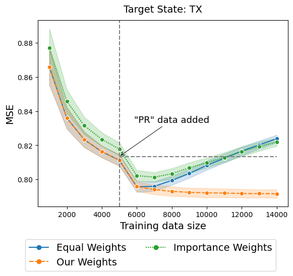
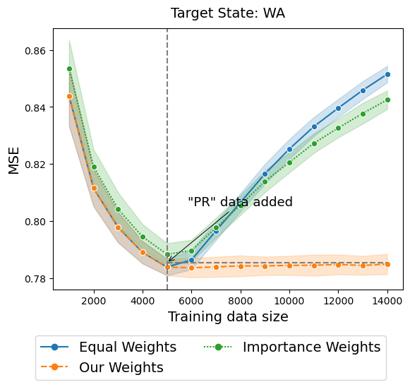
Figure 3: MSE results of the XGBoost when the training data is initially sourced from CA and then sourced from PR. The dashed vertical line indicates the point when PR data started to be added. The blue line is when samples are equally weighted, and the green line is when samples are weighted based on importance weights. The orange line is when samples receive distribution-specific weights using our proposed method.

For the target TX, as we include the PR data, the Mean Squared Error (MSE) initially drops for all the methods. However, as more data from PR is added, the MSE starts to increase for both methods with equal weights and importance weights. In contrast, our method demonstrates robustness, with the MSE decreasing after including PR data and staying consistently low, even when the PR source becomes dominant in the training data set. Turning to the target WA, for both methods with equal weights and importance weights, adding data sourced from PR results in a straightforward increase in MSE. In contrast, our method assigns weights close to 0 for samples originating from PR, preventing significant performance degradation.

6 Discussion

In many practical settings, there is a distribution shift between the training and the target distribution. Existing distribution shift models fall into two categories. One category, which we term “sparse distribution shift”, assumes that the shift affects specific parts of the data generation process while leaving other parts invariant. Existing methods attempt to re-weight training samples to match the target distribution or learn invariant representations of features. The second category considers worst-case distributional shifts. More specifically, they consider the worst-case behavior of a statistical functional over a fixed neighborhood of the model based on the distributional distance. This often requires knowledge of the strength and shape of the perturbations.

In contrast, we consider random dense distributional shifts, where the shift arises as the superposition of many small random changes. We have found that the random perturbation model can be useful in modeling empirical phenomena observed in Figure 1. Moreover, we see that even when the overlap assumptions seem to be violated (when the reweighing approach fails), or when the distribution shift appears large in Kullback-Leibler divergence, the random perturbation model may still be appropriate and useful. Under the random distributional perturbation model, we establish foundations for transfer learning and generalization.

Our method shares methodological similarities with synthetic controls. While synthetic controls are typically applied to panel data under the assumption of a linear factor model, our procedure can be applied to model distribution shifts of any type of data (discrete, continuous, ordinal) with or without time structure. Furthermore, our method justifies the linearity in synthetic control methods under random distributional shifts, rather than assuming a linear factor model. The random distributional shift assumption can be evaluated based on plots in Figure 2. Additionally, we propose a generalization of our procedure to empirical risk minimization.

In practice, perturbations may involve a combination of sparse and dense shifts. In such cases, hybrid approaches (sparse + dense) may be appropriate. We view hybrid models as an important generalization and leave it for future work.

A companion R package, dlm, is available at https://github.com/yujinj/dlm. Our package performs distributional generalization under the random perturbation model. Users can replicate the results in Section 4 with the data and code provided in the package.

7 Acknowledgments

We are grateful for insightful discussions with Naoki Egami, Kevin Guo, Ying Jin, Hongseok Namkoong, and Elizabeth Tipton. This work was supported by Stanford University’s Human-Centered Artificial Intelligence (HAI) Hoffman-Yee Grant, and by the Dieter Schwarz Foundation.

Appendix

Appendix A Proof of Theorem 1

A.1 Extended Theorem 1

In the following, we present the extended version of Theorem 1. Note that we get Theorem 1 in the main text by defining $\phi(D)=(\phi_{1}(D),\dots,\phi_{K}(D))^{\intercal}$.

Extended Theorem 1.

Under the assumptions of Theorem 1, for any Borel measurable square-integrable function $\phi:\mathcal{D}\xrightarrow[]{}\mathbb{R}^{L}$, we have

$$\sqrt{m}\left(\begin{pmatrix}\frac{1}{n_{1}}\sum_{i=1}^{n_{1}}\phi(D_{1i})\\ \vdots\\ \frac{1}{n_{K}}\sum_{i=1}^{n_{K}}\phi(D_{Ki})\end{pmatrix}-\begin{pmatrix}\mathbb{E}^{0}[\phi(D)]\\ \vdots\\ \mathbb{E}^{0}[\phi(D)]\end{pmatrix}\right)\xrightarrow[]{d}N\left(0,\Sigma^{W}\otimes\text{Var}_{\mathbb{P}^{0}}({\phi}(D))\right),$$ (12)

where $\Sigma^{W}\in\mathbb{R}^{K\times K}$ is

$$(\Sigma^{W})_{ij}=\frac{Cov(W^{i},W^{j})}{E[W^{i}]E[W^{j}]}.$$

Here, $\otimes$ denotes a kronecker product. Note that $\Sigma^{W}\otimes\text{Var}_{\mathbb{P}^{0}}({\phi}(D))$ can be written as

$$\left[\begin{array}[]{c@{}c:c:c:c}&\Sigma^{W}_{11}\cdot\text{Var}_{\mathbb{P}^{0}}({\phi}(D))&\Sigma^{W}_{12}\cdot\text{Var}_{\mathbb{P}^{0}}({\phi}(D))&\cdots&\Sigma^{W}_{1K}\cdot\text{Var}_{\mathbb{P}^{0}}({\phi}(D))\\ \hdashline&\Sigma^{W}_{21}\cdot\text{Var}_{\mathbb{P}^{0}}({\phi}(D))&\Sigma^{W}_{22}\cdot\text{Var}_{\mathbb{P}^{0}}({\phi}(D))&\cdots&\Sigma^{W}_{2K}\cdot\text{Var}_{\mathbb{P}^{0}}({\phi}(D))\\ \cdashline{1-5}&{\vdots}&{\vdots}&&{\vdots}\\ \cdashline{1-5}&\Sigma^{W}_{K1}\cdot\text{Var}_{\mathbb{P}^{0}}({\phi}(D))&\Sigma^{W}_{K2}\cdot\text{Var}_{\mathbb{P}^{0}}({\phi}(D))&\cdots&\Sigma^{W}_{KK}\cdot\text{Var}_{\mathbb{P}^{0}}({\phi}(D))\\ \end{array}\right].$$

In the following, we prove Theorem 1. From the proof, we can get Extended Theorem 1 by considering

$$(\hat{\mathbb{E}}^{1}[\phi_{1}(D)],\dots,\hat{\mathbb{E}}^{1}[\phi_{L}(D)],\hat{\mathbb{E}}^{2}[\phi_{1}(D)],\dots,\hat{\mathbb{E}}^{2}[\phi_{L}(D)],\dots\dots,\hat{\mathbb{E}}^{K}[\phi_{1}(D)],\dots,\hat{\mathbb{E}}^{K}[\phi_{L}(D)]),$$

where $\phi(D)=(\phi_{1}(D),\dots,\phi_{L}(D))^{\intercal}\in\mathbb{R}^{L}$.

A.2 Auxiliary Lemma for Theorem 1

Let us first state an auxiliary lemma that will turn out helpful for proving Theorem 1.

Lemma 1.

Let the assumptions of Theorem 1 hold. For any bounded measurable $\phi_{1},\dots,\phi_{K}:\mathcal{D}\xrightarrow[]{}\mathbb{R}$, we have that

$$\sqrt{m}\left(\begin{pmatrix}\mathbb{E}^{1}[\phi_{1}(D)]\\ \vdots\\ \mathbb{E}^{k}[\phi_{K}(D)]\end{pmatrix}-\begin{pmatrix}\mathbb{E}^{0}[\phi_{1}(D)]\\ \vdots\\ \mathbb{E}^{0}[\phi_{K}(D)]\end{pmatrix}\right)\xrightarrow{d}N\left(0,\Sigma^{W}\odot\text{Var}(\overrightarrow{\phi}(D))\right)$$

where $(\Sigma^{W})_{ij}=\frac{Cov(W^{i},W^{j})}{E[W^{i}]E[W^{j}]}$ and $\overrightarrow{\phi}(D)=(\phi_{1}(D),\dots,\phi_{K}(D))^{\intercal}$.

Proof.

Let $\psi_{k}=\phi_{k}\circ h$. Without loss of generality, assume that $\mathbb{E}^{0}[\psi_{k}(U)]=0$ for $k=1,\dots,K$. Note that

$$\sqrt{m}(\mathbb{E}^{k}[\psi_{k}(U)]-\mathbb{E}^{0}[\psi_{k}(U)])=\frac{\sqrt{m}\sum_{j=1}^{m}\int_{x\in I_{j}}\psi_{k}(x)dx\cdot(W^{k}_{j}-E[W^{k}])}{\sum_{j=1}^{m}W^{k}_{j}/m}.$$

Let

$$Y_{m,j}:=\sqrt{m}\begin{pmatrix}\int_{x\in I_{j}}\psi_{1}(x)dx\cdot(W^{1}_{j}-E[W^{1}])\\ \vdots\\ \int_{x\in I_{j}}\psi_{K}(x)dx\cdot(W^{K}_{j}-E[W^{K}])\end{pmatrix}.$$

First, note that

$$E[Y_{m,j}]=0$$ (13)

for all $j$. As the second step, we want to show that

$$\sum_{j=1}^{m}\text{Cov}(Y_{m,j})\xrightarrow[]{}\text{Var}(\overrightarrow{W})\odot\text{Var}_{\mathbb{P}^{0}}(\overrightarrow{\psi}(U)),$$ (14)

where $\overrightarrow{W}=(W^{1},\dots,W^{K})^{\intercal}$, $\overrightarrow{\psi}(U)=(\psi_{1}(U),\dots,\psi_{K}(U))^{\intercal}$, and $\odot$ is an element-wise multiplication. For any $f\in L^{2}([0,1])$, define $\Pi_{m}(f)$ as

$$\Pi_{m}(f)(x)=\sum_{j=1}^{m}\left(m\int_{x\in I_{j}}f(x)dx\right)\cdot I(x\in I_{j}).$$

Then, we have

$$\Bigg{|}\left(\sum_{j=1}^{m}\text{Cov}(Y_{m,j})-\text{Var}(\overrightarrow{W})\odot\text{Var}_{\mathbb{P}^{0}}(\overrightarrow{\psi}(U))\right)_{kk^{\prime}}\Bigg{|}$$

$$\quad\quad\quad\quad=\Bigg{|}\left(m\sum_{j=1}^{m}\int_{x\in I_{j}}\psi_{k}(x)dx\int_{x\in I_{j}}\psi_{k^{\prime}}(x)dx-\sum_{j=1}^{m}\int_{x\in I_{j}}\psi_{k}(x)\psi_{k^{\prime}}(x)dx\right)\cdot\text{Cov}(W^{k},W^{k^{\prime}})\Bigg{|}$$

$$\quad\quad\quad\quad\leq||\psi_{k}||_{2}||\psi_{k^{\prime}}-\Pi_{m}(\psi_{k^{\prime}})||_{2}\cdot|\text{Cov}(W^{k},W^{k^{\prime}})|\xrightarrow[]{}0$$

for $1\leq k,k^{\prime}\leq K$ as $m$ goes to infinity. This is because any bounded function can be approximated by a sequence of step functions of the form $\sum_{j=1}^{m}b_{j}I(x\in I_{j})$. Next we will show that for any $\epsilon>0$,

$$g_{m}(\epsilon)=\sum_{j=1}^{m}E[||Y_{m,j}||_{2}^{2};||Y_{m,j}||_{2}\geq\epsilon]\xrightarrow[]{}0.$$ (15)

Let $||\psi_{1}||_{\infty},\dots,||\psi_{K}||_{\infty}\leq B$. Then this is implied by the dominated convergence theorem as

$$\sum_{j=1}^{m}E[||Y_{m,j}||_{2}^{2};||Y_{m,j}||_{2}\geq\epsilon] \leq B^{2}E[||\overrightarrow{W}-E[\overrightarrow{W}]||_{2}^{2}I(B||\overrightarrow{W}-E[\overrightarrow{W}]||_{2}/\sqrt{m}\geq\epsilon)]\xrightarrow[]{}0.$$ (16)

Combining equations (13), (14), and (15), we can apply multivariate Lindeberg’s CLT. Together with Slutsky’s theorem, we have

$$\sqrt{m}\left(\begin{pmatrix}\mathbb{E}^{1}[\phi_{1}(D]\\ \vdots\\ \mathbb{E}^{k}[\phi_{K}(D)]\end{pmatrix}-\begin{pmatrix}\mathbb{E}^{0}[\phi_{1}(D]\\ \vdots\\ \mathbb{E}^{0}[\phi_{K}(D)]\end{pmatrix}\right) =\sum_{j=1}^{m}Y_{m,j}\odot\begin{pmatrix}1/(\sum_{j=1}^{m}W_{j}^{1}/m)\\ \vdots\\ 1/(\sum_{j=1}^{m}W_{j}^{K}/m)\end{pmatrix}$$

$$\xrightarrow[]{d}N\left(0,\Sigma^{W}\odot\text{Var}_{\mathbb{P}^{0}}(\overrightarrow{\phi}(D))\right)$$

where $\Sigma^{W}_{ij}=\frac{Cov(W^{i},W^{j})}{E[W^{i}]E[W^{j}]}$. This completes the proof. ∎

A.3 Proof of Theorem 1

Proof.

For any $\phi_{k}\in L^{2}(\mathbb{P})$ and for any given $\epsilon>0$, there exits a bounded function $\phi_{k}^{B}$ such that $\mathbb{E}^{0}[\phi_{k}(D)]=\mathbb{E}^{0}[\phi_{k}^{B}(D)]$ and $||\phi_{k}-\phi_{k}^{B}||_{L^{2}(\mathbb{P}^{0})}<\epsilon$ for $k=1,\dots,K$. Then,

$$\sqrt{m}\left(\begin{pmatrix}\frac{1}{n_{1}}\sum_{i=1}^{n_{1}}\phi_{1}(D_{1i})\\ \vdots\\ \frac{1}{n_{K}}\sum_{i=1}^{n_{K}}\phi_{K}(D_{Ki})\end{pmatrix}-\begin{pmatrix}\mathbb{E}^{0}[\phi_{1}(D]\\ \vdots\\ \mathbb{E}^{0}[\phi_{K}(D)]\end{pmatrix}\right)$$

$$\quad\quad\quad\quad\quad\quad\quad\quad\quad=\sqrt{m}\left(\begin{pmatrix}\frac{1}{n_{1}}\sum_{i=1}^{n_{1}}\phi_{1}(D_{1i})\\ \vdots\\ \frac{1}{n_{K}}\sum_{i=1}^{n_{K}}\phi_{K}(D_{Ki})\end{pmatrix}-\begin{pmatrix}\mathbb{E}^{1}[\phi_{1}(D]\\ \vdots\\ \mathbb{E}^{k}[\phi_{K}(D)]\end{pmatrix}\right)$$ (a)

$$\quad\quad\quad\quad\quad\quad\quad\quad\quad+\sqrt{m}\left(\begin{pmatrix}\mathbb{E}^{1}[\phi_{1}(D)]\\ \vdots\\ \mathbb{E}^{k}[\phi_{K}(D)]\end{pmatrix}-\begin{pmatrix}\mathbb{E}^{1}[\phi_{1}^{B}(D)]\\ \vdots\\ \mathbb{E}^{k}[\phi_{K}^{B}(D)]\end{pmatrix}\right)$$ (b)

$$\quad\quad\quad\quad\quad\quad\quad\quad\quad+\sqrt{m}\left(\begin{pmatrix}\mathbb{E}^{1}[\phi_{1}^{B}(D)]\\ \vdots\\ \mathbb{E}^{k}[\phi_{K}^{B}(D)]\end{pmatrix}-\begin{pmatrix}\mathbb{E}^{0}[\phi_{1}^{B}(D)]\\ \vdots\\ \mathbb{E}^{0}[\phi_{K}^{B}(D)]\end{pmatrix}\right).$$ (c)

Note that for any $\epsilon^{\prime}>0$ and for $k=1,\dots,K$,

$$P\left(\sqrt{m}\Bigg{|}\frac{1}{n_{k}}\sum_{i=1}^{n_{k}}\phi_{k}(D_{ki})-\mathbb{E}^{k}[\phi_{k}(D)]\Bigg{|}>\epsilon^{\prime}\right) =E\left(P\left(\Bigg{|}\frac{1}{n_{k}}\sum_{i=1}^{n_{k}}\phi_{k}(D_{ki})-\mathbb{E}^{k}[\phi_{k}(D)]\Bigg{|}>\frac{\epsilon^{\prime}}{\sqrt{m}}\text{ }\Bigg{|}\text{ }W_{k}\right)\right)$$

$$\leq E\left(\frac{\mathbb{E}^{k}[\phi_{k}^{2}(D)]}{\epsilon^{\prime 2}}\right)\cdot\frac{m}{n_{k}}=\frac{\mathbb{E}^{0}[\phi_{k}^{2}(D)]}{\epsilon^{\prime 2}}\cdot\frac{m}{n_{k}}\xrightarrow[]{}0,$$

as the distributional uncertainty is of higher order than the sampling uncertainty. Therefore, (a) $=o_{p}(1)$. Next let us investigate (b). Recall that with $\psi_{k}=(\phi_{k}-\phi_{k}^{B})\circ h$,

$$\sqrt{m}(\mathbb{E}^{k}[\phi_{k}(D)]-\mathbb{E}^{k}[\phi_{k}^{B}(D)]) =\frac{\sqrt{m}\sum_{j=1}^{m}\int_{x\in I_{j}}\psi_{k}(x)dx\cdot(W_{j}^{k}-E[W^{k}])}{\sum_{j=1}^{m}W_{j}^{k}/m}.$$

The variance of the numerator is bounded as

$$\text{Var}(W^{k})\sum_{j=1}^{m}m\left(\int_{x\in I_{j}}\psi_{k}(x)dx\right)^{2} \leq\text{Var}(W^{k})\sum_{j=1}^{m}\int_{x\in I_{j}}\psi_{k}^{2}(x)dx$$

$$=\text{Var}(W^{k})\mathbb{E}^{0}[\psi_{k}^{2}(U)]$$

$$<\text{Var}(W^{k})\cdot\epsilon^{2}$$

where the first inequality holds by Jensen’s inequality with $m\int_{x\in I_{j}}dx=1$. The denominator converges in probability to $E[W^{k}]$. Therefore, we can write

$$\sqrt{m}(\mathbb{E}^{k}[\phi_{k}(D)]-\mathbb{E}^{k}[\phi_{k}^{B}(D)])=\frac{\sqrt{m}\sum_{j=1}^{m}\int_{x\in I_{j}}\psi_{k}(x)dx\cdot(W_{j}^{k}-E[W^{k}])}{E[W^{k}]}+s_{n,k}$$

where $s_{n,k}$ is $o_{p}(1)$. Combining results, for $s_{n}=(s_{n,1},\dots,s_{n,K})^{\intercal}$, we have that $E[\eqref{eq:b}-s_{n}]=0$ and

$$||\text{Var}_{P}(\eqref{eq:b}-s_{n})||_{\infty}\leq\frac{||\text{Var}(\overrightarrow{W})||_{\infty}}{\min_{k}E^{2}[W^{k}]}\cdot\epsilon^{2}.$$

From Lemma 1, we know that

$$\eqref{eq:c}\xrightarrow[]{d}N\left(0,\Sigma^{W}\odot\text{Var}_{\mathbb{P}^{0}}\left(\overrightarrow{\phi^{B}}(D)\right)\right).$$

Let $||\phi_{1}^{B}||_{2},\dots,||\phi_{K}^{B}||_{2},||\phi_{1}||_{2},\dots,||\phi_{K}||_{2}\leq M$. Note that for any $1\leq k,k^{\prime}\leq K$,

$$2|\mathbb{E}^{0}[\phi_{k}\phi_{k^{\prime}}]-\mathbb{E}^{0}[\phi_{k}^{B}\phi_{k^{\prime}}^{B}]| \leq|\mathbb{E}^{0}[(\phi_{k}-\phi_{k}^{B})(\phi_{k^{\prime}}+\phi_{k^{\prime}}^{B})]|+|\mathbb{E}^{0}[(\phi_{k}+\phi_{k}^{B})(\phi_{k^{\prime}}-\phi_{k^{\prime}}^{B})]|$$

$$\leq 2M(||\phi_{k}-\phi_{k}^{B}||_{2}+||\phi_{k^{\prime}}-\phi_{k^{\prime}}^{B}||_{2})\leq 4M\cdot\epsilon.$$

Therefore,

$$\Big{|}\Big{|}\text{Var}_{\mathbb{P}^{0}}(\overrightarrow{\phi}(D))-\text{Var}_{\mathbb{P}^{0}}(\overrightarrow{\phi^{B}}(D))\Big{|}\Big{|}_{\infty}\leq 2M\cdot\epsilon.$$

Combining results, we have

$$\eqref{eq:a}+\eqref{eq:b}+\eqref{eq:c} \stackrel{{\scriptstyle d}}{{=}}N\left(0,\Sigma^{W}\odot\text{Var}_{\mathbb{P}^{0}}(\overrightarrow{\phi}(D))\right)+o_{p}(1)$$

$$+(\eqref{eq:b}-s_{n})+N\left(0,\Sigma^{W}\odot\left(\text{Var}_{\mathbb{P}^{0}}(\overrightarrow{\phi}(D))-\text{Var}_{\mathbb{P}^{0}}(\overrightarrow{\phi^{B}}(D))\right)\right)$$

$$=N\left(0,\Sigma^{W}\odot\text{Var}_{\mathbb{P}^{0}}(\overrightarrow{\phi}(D))\right)+O_{p}(\epsilon)+o_{p}(1).$$

Note that all the results hold for arbitrary $\epsilon>0$. This completes the proof. ∎

A.4 Remark 1

From Extended Theorem 1 with $K+1$ data sets and $\Sigma^{W}\in\mathbb{R}^{(K+1)\times(K+1)}$, and considering that the sampling uncertainty is of low order than distributional uncertainty, for any Borel measurable square-integrable function $\phi:\mathcal{D}\xrightarrow[]{}\mathbb{R}^{L}$, we have

$$\sqrt{m}\left(\begin{pmatrix}\frac{1}{n_{1}}\sum_{i=1}^{n_{1}}\phi(D_{1i})\\ \vdots\\ \frac{1}{n_{K}}\sum_{i=1}^{n_{K}}\phi(D_{Ki})\end{pmatrix}-\begin{pmatrix}\mathbb{E}^{K+1}[\phi(D)]\\ \vdots\\ \mathbb{E}^{K+1}[\phi(D)]\end{pmatrix}\right)\xrightarrow[]{d}N\left(0,(A\Sigma^{W}A^{\intercal})\otimes\text{Var}_{\mathbb{P}^{0}}({\phi}(D))\right),$$ (17)

where

$$A=\begin{pmatrix}1&0&\dots&0&-1\\ 0&1&\dots&0&-1\\ \vdots&\vdots&&\vdots&\vdots\\ 0&0&\dots&1&-1\end{pmatrix}\in\mathbb{R}^{K\times(K+1)}.$$

Therefore, with $\mathbb{P}^{K+1}$ as a new target distribution, we still have Extended Theorem 1 but with a different distributional covariance matrix $A\Sigma^{W}A^{\intercal}$.

A.5 Remark 2

Note that $\widehat{\text{Var}}_{\mathbb{P}^{0}}(\phi(D))$ is an empirical variance of $\phi$ on the pooled donor data $\{(D_{ki})_{i=1}^{n_{k}}\}_{k=1}^{K}$ and can be written as

$$\widehat{\text{Var}}_{\mathbb{P}^{0}}(\phi(D))= \sum_{k=1}^{K}\frac{n_{k}}{n}\frac{1}{n_{k}}\sum_{i=1}^{n_{k}}\phi(D_{ki})\phi(D_{ki})^{\intercal}-\left(\sum_{k=1}^{K}\frac{n_{k}}{n}\frac{1}{n_{k}}\sum_{i=1}^{n_{k}}\phi(D_{ki})\right)\left(\sum_{k=1}^{K}\frac{n_{k}}{n}\frac{1}{n_{k}}\sum_{i=1}^{n_{k}}\phi(D_{ki})\right)^{\intercal}.$$

where $n=n_{1}+\dots+n_{K}$. As $\phi$ has a finite fourth moment, by Theorem 1, we have that

$$\widehat{\text{Var}}_{\mathbb{P}^{0}}(\phi(D)) =\sum_{k=1}^{K}\frac{n_{k}}{n}\left(\mathbb{E}^{0}[\phi(D)\phi(D)^{\intercal}]+o_{p}(1)\right)$$

$$-\left(\sum_{k=1}^{K}\frac{n_{k}}{n}\left(\mathbb{E}^{0}[\phi(D)]+o_{p}(1)\right)\right)\left(\sum_{k=1}^{K}\frac{n_{k}}{n}\left(\mathbb{E}^{0}[\phi(D)]+o_{p}(1)\right)\right)^{\intercal}$$

$$=\text{Var}_{\mathbb{P}^{0}}(\phi(D))+o_{p}(1).$$

Appendix B Proof of Theorem 2

Define the feature matrix before reparametrization as

$$\Phi=\begin{pmatrix}\hat{\mathbb{E}}^{1}[\phi_{1}]-\hat{\mathbb{E}}^{0}[\phi_{1}]&\dots&\hat{\mathbb{E}}^{K}[\phi_{1}]-\hat{\mathbb{E}}^{0}[\phi_{1}]\\ \vdots&&\vdots\\ \hat{\mathbb{E}}^{1}[\phi_{L}]-\hat{\mathbb{E}}^{0}[\phi_{L}]&\dots&\hat{\mathbb{E}}^{K}[\phi_{L}]-\hat{\mathbb{E}}^{0}[\phi_{L}]\end{pmatrix}\in\mathbb{R}^{L\times K},$$

where the $\ell$-th row is defined as $\Phi_{\ell}$.

By Theorem 1 and using that the sampling uncertainty is of low order than distributional uncertainty, we have

$$\sqrt{m}\Phi_{\ell}:=\sqrt{m}\begin{pmatrix}\hat{\mathbb{E}}^{1}[\phi_{\ell}]-\hat{\mathbb{E}}^{0}[\phi_{\ell}]\\ \vdots\\ \hat{\mathbb{E}}^{K}[\phi_{\ell}]-\hat{\mathbb{E}}^{0}[\phi_{\ell}]\end{pmatrix}\stackrel{{\scriptstyle d}}{{=}}\bm{Z}_{\ell}+o_{p}(1)$$

where $\bm{Z}_{1},\dots,\bm{Z}_{L}\in\mathbb{R}^{K}$ are i.i.d Gaussian random variables following $N(0,\Sigma^{W})$. Let $\bm{Z}\in\mathbb{R}^{L\times K}$ be a matrix in which the $\ell$-th row is $\bm{Z}_{\ell}$.

Note that

$$\hat{\beta}=\operatorname*{argmin}_{\beta:\beta^{\intercal}1=1}\beta^{\intercal}\left(\sum_{\ell=1}^{L}\Phi_{\ell}\Phi_{\ell}^{\intercal}\right)\beta=\arg\min_{\beta:\beta^{\intercal}1=1}\beta^{\intercal}\bm{\Phi}^{\intercal}\bm{\Phi}\beta.$$

The closed form of $\hat{\beta}$ is known as

$$\hat{\beta}=\frac{(\bm{\Phi}^{\intercal}\bm{\Phi})^{-1}\bm{1}}{\bm{1}^{\intercal}(\bm{\Phi}^{\intercal}\bm{\Phi})^{-1}\bm{1}}\stackrel{{\scriptstyle d}}{{=}}\frac{(\bm{Z}^{\intercal}\bm{Z})^{-1}\bm{1}}{\bm{1}^{\intercal}(\bm{Z}^{\intercal}\bm{Z})^{-1}\bm{1}}+o_{p}(1).$$

We write $\hat{\beta}_{Z}=\frac{(\bm{Z}^{\intercal}\bm{Z})^{-1}\bm{1}}{\bm{1}^{\intercal}(\bm{Z}^{\intercal}\bm{Z})^{-1}\bm{1}}$. Moreover, the closed form of $\beta^{*}$ is

$$\beta^{*}=\operatorname*{argmin}_{\beta:\beta^{\intercal}1=1}\beta^{\intercal}\Sigma^{W}\beta=\frac{(\Sigma^{W})^{-1}\bm{1}}{\bm{1}^{\intercal}(\Sigma^{W})^{-1}\bm{1}}.$$

Let $Q$ be a $p\times(K-1)$ non-random matrix with $\text{rank}(Q)=p\leq K-1$. Let $\tilde{Q}=(Q^{\prime\intercal},\bm{1})^{\intercal}\in\mathbb{R}^{(p+1)\times K}$ where

$$Q^{\prime}=Q\begin{pmatrix}\bm{I}_{(K-1)\times(K-1)}&\bm{0}_{(K-1)\times 1}\end{pmatrix}\in\mathbb{R}^{p\times K}.$$

Note that the $\text{rank}(\tilde{Q})=p+1\leq K$. Define $\tilde{S}:=\tilde{Q}(\bm{Z}^{\intercal}\bm{Z})^{-1}\tilde{Q}^{\intercal}$ where

$$\tilde{S}=\begin{pmatrix}\tilde{S}_{11}&\tilde{S}_{12}\\ \tilde{S}_{21}&\tilde{S}_{22}\end{pmatrix}=\begin{pmatrix}Q^{\prime}(\bm{Z}^{\intercal}\bm{Z})^{-1}Q^{\prime\intercal}&Q^{\prime}(\bm{Z}^{\intercal}\bm{Z})^{-1}\bm{1}\\ \bm{1}^{\intercal}(\bm{Z}^{\intercal}\bm{Z})^{-1}Q^{\prime\intercal}&\bm{1}^{\intercal}(\bm{Z}^{\intercal}\bm{Z})^{-1}\bm{1}.\end{pmatrix}$$

Similarly, let $\tilde{P}:=\tilde{Q}(\Sigma^{W})^{-1}\tilde{Q}^{\intercal}$ where $\tilde{P}_{11}=Q^{\prime}(\Sigma^{W})^{-1}Q^{\prime\intercal},\tilde{P}_{12}=Q^{\prime}(\Sigma^{W})^{-1}\bm{1},$ and $\tilde{P}_{22}=\bm{1}^{\intercal}(\Sigma^{W})^{-1}\bm{1}$.

Results from Multivariate Statistical Theory.

Note that $\bm{Z}^{\intercal}\bm{Z}\sim\text{Wish}_{K}(L;\Sigma^{W})$ which is the Wishart distribution with a degree of freedom $L$ and a scale matrix $\Sigma^{W}$. By Theorem 3.2.11 and 3.6 in Muirhead [1982], we have

$$\tilde{S}\sim W_{p+1}^{-1}(L-K+2p+3;\tilde{P}).$$

which is the inverse-Wishart distribution with a degree of freedom $L-K+2p+3$ and a scale matrix $\tilde{P}$. By Theorem 3 (b) and (d) of Bodnar and Okhrin [2008], we have that

$$\tilde{S}_{12}\tilde{S}_{22}^{-1}|\tilde{S}_{11.2}\sim N(\tilde{P}_{12}\tilde{P}_{22}^{-1},\tilde{S}_{11.2}\otimes\tilde{P}_{22}^{-1}).$$

Therefore, we get

$$\tilde{P}_{22}^{1/2}\tilde{S}_{11.2}^{-1/2}\left(\tilde{S}_{12}\tilde{S}_{22}^{-1}-\tilde{P}_{12}\tilde{P}_{22}^{-1}\right)|\tilde{S}_{11.2}\sim N(0,\bm{I}).$$

The right hand side does not depend on $\tilde{S}_{11.2}$ anymore. Therefore, we have

$$\tilde{P}_{22}^{1/2}\tilde{S}_{11.2}^{-1/2}\left(Q(\hat{\beta}_{Z})_{1:(K-1)}-Q{\beta}^{*}_{1:(K-1)}\right)\sim N(\bm{0},\bm{I}).$$ (18)

By Theorem 3.2.12 in Muirhead [1982], we have

$$\frac{\tilde{P}_{22}}{\tilde{S}_{22}}=\frac{\bm{1}^{\intercal}(\Sigma^{W})^{-1}\bm{1}}{\bm{1}^{\intercal}(Z^{\intercal}Z)^{-1}\bm{1}}\sim\chi^{2}(L-K+1).$$

By Theorem 3 (e) of Bodnar and Okhrin [2008], $\tilde{S}_{22}$ is independent of $\tilde{S}_{12}\tilde{S}_{22}^{-1}$ and $\tilde{S}_{11.2}$. Hence, we get

$$\sqrt{L-K+1}\cdot\tilde{S}_{22}^{1/2}\tilde{S}_{11.2}^{-1/2}\left(Q(\hat{\beta}_{Z})_{1:(K-1)}-Q{\beta}^{*}_{1:(K-1)}\right)\sim t_{p}(L-K+1;\bm{0},\bm{I}),$$

where $t_{p}(L-K+1;\bm{0},\bm{I})$ is $p$-dimensional (centered) $t$-distribution with $L-K+1$ degrees of freedom. Now using $\Phi=\bm{Z}/\sqrt{m}+o_{p}(1/\sqrt{m})$ from Theorem 1, we get

$$\sqrt{L-K+1}\sqrt{\bm{1}^{\intercal}(\bm{\Phi}^{\intercal}\bm{\Phi})^{-1}\bm{1}}\cdot\left[QRQ^{\intercal}\right]^{-1/2}\left(Q\hat{\beta}_{1:(K-1)}-Q{\beta}^{*}_{1:(K-1)}\right)$$ (19)

$$\stackrel{{\scriptstyle d}}{{=}}t_{p}(L-K+1;\bm{0},\bm{I})+o_{p}(1).$$ (20)

where

$$R=\begin{pmatrix}\bm{I}_{(K-1)\times(K-1)}&\bm{0}_{(K-1)\times 1}\end{pmatrix}\left((\bm{\Phi}^{\intercal}\bm{\Phi})^{-1}-\frac{(\bm{\Phi}^{\intercal}\bm{\Phi})^{-1}\bm{1}\bm{1}^{\intercal}(\bm{\Phi}^{\intercal}\bm{\Phi})^{-1}}{\bm{1}^{\intercal}(\bm{\Phi}^{\intercal}\bm{\Phi})^{-1}\bm{1}}\right)\begin{pmatrix}\bm{I}_{(K-1)\times(K-1)}&\bm{0}_{(K-1)\times 1}\end{pmatrix}^{\intercal}.$$

Connection with Reparametrized Linear Regression.

In this part, we will show that

$$(\tilde{\bm{\Phi}}^{\intercal}\tilde{\bm{\Phi}})^{-1}=R.$$ (21)

Using the closed form of $\hat{\beta}$, we have that

$$(L-K+1)\cdot\hat{\sigma}^{2}=\hat{\beta}^{\intercal}\Phi^{\intercal}\Phi\hat{\beta}=\frac{1}{\bm{1}^{\intercal}(\Phi^{\intercal}\Phi)^{-1}\bm{1}}.$$ (22)

Then combining (20), (21), and (22), we have

$$\left(Q(\tilde{\Phi}^{\intercal}\tilde{\Phi})^{-1}\hat{\sigma}^{2}Q^{\intercal}\right)^{-\frac{1}{2}}\left(Q\hat{\beta}_{1:(K-1)}-Q\beta^{*}_{1:(K-1)}\right)\stackrel{{\scriptstyle d}}{{=}}t_{p}(L-K+1;\bm{0},\bm{I})+o_{p}(1).$$

Note that this is a more general version of Theorem 2. By letting $Q$ be an $(K-1)\times(K-1)$ identity matrix, we have Theorem 2. For the simplicity of notation, let $V=\bm{\Phi}^{\intercal}\bm{\Phi}$. Note that

$$\tilde{\bm{\Phi}}^{\intercal}\tilde{\bm{\Phi}} =\begin{pmatrix}\bm{I}_{(K-1)\times(K-1)}&-\bm{1}\end{pmatrix}\begin{pmatrix}V_{11}&V_{12}\\ V_{12}^{\intercal}&V_{22}\end{pmatrix}\begin{pmatrix}\bm{I}_{(K-1)\times(K-1)}&-\bm{1}\end{pmatrix}^{\intercal}$$

$$=V_{11}-\bm{1}V_{12}^{\intercal}-V_{12}\bm{1}^{\intercal}+\bm{1}V_{22}\bm{1}^{\intercal}$$

where $V_{22}\in\mathbb{R}$ and $\bm{1}\in\mathbb{R}^{(K-1)\times 1}$. Then, by applying Sherman-Morrison lemma, we have

$$(\tilde{\bm{\Phi}}^{\intercal}\tilde{\bm{\Phi}})^{-1} =\left(V_{11.2}+V_{12}V_{22}^{-1}V_{12}^{\intercal}-\bm{1}V_{12}^{\intercal}-V_{12}\bm{1}^{\intercal}+\bm{1}V_{22}\bm{1}^{\intercal}\right)^{-1}$$

$$=\left(V_{11.2}+\left(V_{12}V_{22}^{-1/2}-V_{22}^{1/2}\bm{1}\right)\left(V_{12}V_{22}^{-1/2}-V_{22}^{1/2}\bm{1}\right)^{\intercal}\right)^{-1}$$

$$=V_{11.2}^{-1}-\frac{V_{11.2}^{-1}\left(V_{12}V_{22}^{-1/2}-V_{22}^{1/2}\bm{1}\right)\left(V_{12}V_{22}^{-1/2}-V_{22}^{1/2}\bm{1}\right)^{\intercal}V_{11.2}^{-1}}{1+\left(V_{12}V_{22}^{-1/2}-V_{22}^{1/2}\bm{1}\right)^{\intercal}V_{11.2}^{-1}\left(V_{12}V_{22}^{-1/2}-V_{22}^{1/2}\bm{1}\right)}.$$

By using the inverse of block matrix as

$$V^{-1}=\begin{pmatrix}V_{11.2}^{-1}&-V_{11.2}^{-1}V_{12}V_{22}^{-1}\\ -V_{22}^{-1}V_{12}^{\intercal}V_{11.2}^{-1}&V_{22}^{-1}+V_{22}^{-1}V_{12}^{\intercal}V_{11.2}^{-1}V_{12}V_{22}^{-1}\end{pmatrix},$$

we also get

$$R=V_{11.2}^{-1}-\frac{V_{11.2}^{-1}\left(V_{12}V_{22}^{-1}-\bm{1}\right)\left(V_{12}V_{22}^{-1}-\bm{1}\right)^{\intercal}V_{11.2}^{-1}}{\bm{1}^{\intercal}V_{11.2}^{-1}\bm{1}-V_{22}^{-1}V_{12}^{\intercal}V_{11.2}^{-1}\bm{1}-\bm{1}^{\intercal}V_{11.2}^{-1}V_{12}V_{22}^{-1}+V_{22}^{-1}+V_{22}^{-1}V_{12}^{\intercal}V_{11.2}^{-1}V_{12}V_{22}^{-1}}.$$

Then, we can easily check that $(\tilde{\bm{\Phi}}^{\intercal}\tilde{\bm{\Phi}})^{-1}=R$. This completes the proof.

Appendix C Confidence Intervals for $\mathbb{E}^{0}[\phi_{0}(D)]$

We will discuss how to form asymptotically valid confidence intervals for $\mathbb{E}^{0}[\phi_{0}(D)]$. Assume that test functions $\phi_{1}(X),\dots,\phi_{L}(X)$ are uncorrelated and have unit variances under $\mathbb{P}^{0}$.

Let’s say $\hat{\beta}$ in (7) is consistent as follows,

$$\hat{\beta}\xrightarrow[]{p}\beta^{*}:=\operatorname*{argmin}_{\beta:\beta^{\intercal}1}\beta^{\intercal}\Sigma^{W}\beta.$$

Then, we have for $\overrightarrow{\hat{\mathbb{E}}[\phi_{0}]}=(\hat{\mathbb{E}}^{1}[\phi_{0}],\dots,\hat{\mathbb{E}}^{K}[\phi_{0}])^{\intercal}$,

$$\sqrt{m}\left(\sum_{k=1}^{K}\hat{\beta}_{k}\hat{\mathbb{E}}^{k}[\phi_{0}]-\mathbb{E}^{0}[\phi_{0}]\right) =\sqrt{m}\left(\hat{\beta}-\beta^{*}\right)^{\intercal}\left(\overrightarrow{\hat{\mathbb{E}}[\phi_{0}]}-\mathbb{1}\cdot\mathbb{E}^{0}[\phi_{0}]\right)$$

$$+\sqrt{m}\text{ }{\beta^{*}}^{\intercal}\left(\overrightarrow{\hat{\mathbb{E}}[\phi_{0}]}-\mathbb{1}\cdot\mathbb{E}^{0}[\phi_{0}]\right)$$

since $\hat{\beta}^{\intercal}\mathbb{1}=1$ and $\beta^{*}{}^{\intercal}\mathbb{1}=1$. By Theorem 1,

$$\sqrt{m}\left(\overrightarrow{\hat{\mathbb{E}}[\phi_{0}]}-\mathbb{1}\cdot\mathbb{E}^{0}[\phi_{0}]\right)\xrightarrow[]{d}N(0,\text{Var}_{\mathbb{P}^{0}}(\phi_{0})\cdot\Sigma^{W}).$$

Therefore,

$$\sqrt{m}\left(\sum_{k=1}^{K}\hat{\beta}_{k}\hat{\mathbb{E}}^{k}[\phi_{0}]-\mathbb{E}^{0}[\phi_{0}]\right) =\sqrt{m}\text{ }{\beta^{*}}^{\intercal}\left(\overrightarrow{\hat{\mathbb{E}}[\phi_{0}]}-\mathbb{1}\cdot\mathbb{E}^{0}[\phi_{0}]\right)+o_{p}(1)$$ (23)

$$\xrightarrow[]{d}N(0,\text{Var}_{\mathbb{P}^{0}}(\phi_{0})\cdot{\beta^{*}}^{\intercal}\Sigma^{W}\beta^{*}).$$ (24)

Then, we can construct confidence interval for $\mathbb{E}^{0}[\phi_{0}]$ as

$$\sum_{k=1}^{K}\hat{\beta}_{k}\hat{\mathbb{E}}^{k}[\phi_{0}]\pm z_{1-\alpha/2}\cdot\sqrt{\text{Var}_{\mathbb{P}^{0}}(\phi_{0})}\cdot\sqrt{\frac{{\beta^{*}}^{\intercal}\Sigma^{W}\beta^{*}}{m}}.$$

How can we obtain a consistent estimator for ${\beta^{*}}^{\intercal}\Sigma^{W}\beta^{*}/m$? By Theorem 1,

$$\hat{\mathbb{E}}^{0}[\phi_{\ell}]-\sum_{k=1}^{K}\beta_{k}^{*}\hat{\mathbb{E}}^{k}[\phi_{\ell}]\text{ }\stackrel{{\scriptstyle d}}{{=}}\text{ }\sqrt{\frac{{\beta^{*}}^{\intercal}\Sigma^{W}\beta^{*}}{m}}\cdot Z_{\ell}+o_{p}(1/\sqrt{m})$$

where $Z_{\ell}$ for $\ell=1,\dots,L$ are independent standard Gaussian variables. Then,

$$\left(\hat{\mathbb{E}}^{0}[\phi_{\ell}]-\sum_{k=1}^{K}\hat{\beta}_{k}\hat{\mathbb{E}}^{k}[\phi_{\ell}]\right)^{2} =\left(\left(\hat{\mathbb{E}}^{0}[\phi_{\ell}]-\sum_{k=1}^{K}\beta^{*}_{k}\hat{\mathbb{E}}^{k}[\phi_{\ell}]\right)+\left(\sum_{k=1}^{K}(\hat{\beta}_{k}-\beta^{*}_{k})(\hat{\mathbb{E}}^{0}[\phi_{\ell}]-\hat{\mathbb{E}}^{k}[\phi_{\ell}])\right)\right)^{2}$$

$$\stackrel{{\scriptstyle d}}{{=}}{\frac{{\beta^{*}}^{\intercal}\Sigma^{W}\beta^{*}}{m}}\cdot Z_{\ell}^{2}+o_{p}(1/m).$$

Therefore, we may estimate ${\beta^{*}}^{\intercal}\Sigma^{W}\beta^{*}/m$ as

$$\frac{1}{L}\sum_{\ell=1}^{L}\left(\mathbb{E}^{0}[\phi_{\ell}]-\sum_{k=1}^{K}\hat{\beta}_{k}\hat{\mathbb{E}}^{k}[\phi_{\ell}]\right)^{2}\stackrel{{\scriptstyle d}}{{=}}{\frac{{\beta^{*}}^{\intercal}\Sigma^{W}\beta^{*}}{m}}\cdot\frac{\chi^{2}(L)}{L}+o_{p}(1/m),$$ (25)

where $\chi^{2}(L)$ is a chi-squared random variable with degrees of freedom $L$. Additionally, in Remark 2, we see that $\widehat{\text{Var}}_{\mathbb{P}^{0}}(\phi_{0}(D))=\text{Var}_{\mathbb{P}^{0}}(\phi_{0}(D))+o_{p}(1)$.

Finally, as $L\xrightarrow[]{}\infty$, we have the consistency of $\hat{\beta}$ and $\chi^{2}(L)/L\xrightarrow[]{p}1$. Combining all the results, we have asymptotically valid ($1-\alpha$) confidence interval as $m\xrightarrow[]{}\infty$ and $L\xrightarrow[]{}\infty$:

$$\sum_{k=1}^{K}\hat{\beta}_{k}\hat{\mathbb{E}}^{k}[\phi_{0}]\pm z_{1-\alpha/2}\cdot\sqrt{\widehat{\text{Var}}_{\mathbb{P}^{0}}(\phi_{0})}\cdot\sqrt{\frac{1}{L}\sum_{\ell=1}^{L}\left(\hat{\mathbb{E}}^{0}[\phi_{\ell}]-\sum_{k=1}^{K}\hat{\beta}_{k}\hat{\mathbb{E}}^{k}[\phi_{\ell}]\right)^{2}}.$$

Appendix D Additional Details in Data Analysis

D.1 Covariance of Test Functions in GTEx Data Analysis

We estimate the sparse inverse covariance matrix of test functions $(\phi_{\ell})_{\ell=1,\dots,L=1000}$ defined in Section 4, using group Lasso with a Python package sklearn.covariance.GraphicalLassoCV. The heatmap of fitted precision matrix is given in Figure 4. As the estimated inverse covariance matrix was close to a diagonal matrix, we did not perform a whitening transformation for the 1000 test functions.

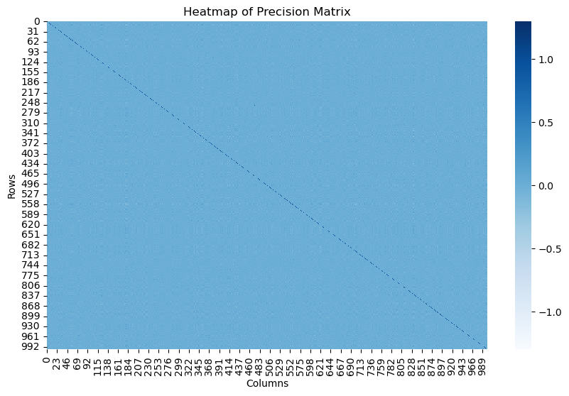
Figure 4: Fitted sparse precision matrix of test functions defined in Section 4 on the GTEx data

D.2 Additional Results for ACS Income Data Analysis

In this section, we provide additional results for ACS income data analysis in Section 5 for 6 randomly selected target states. The results are presented in Figure 5.

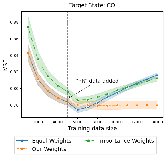
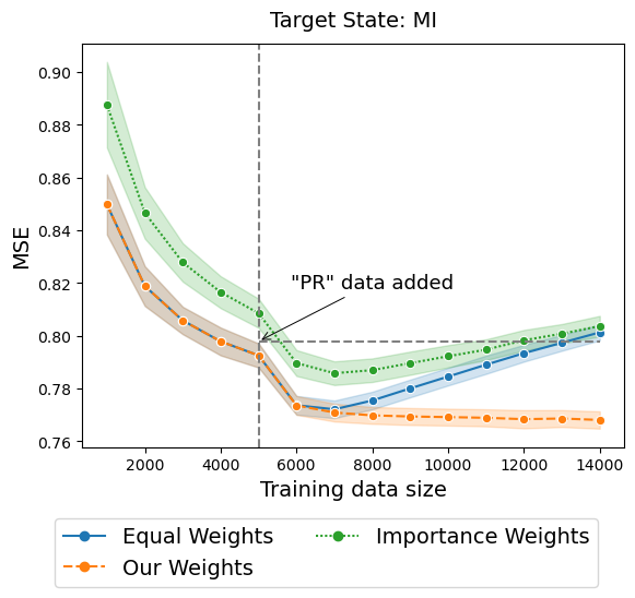
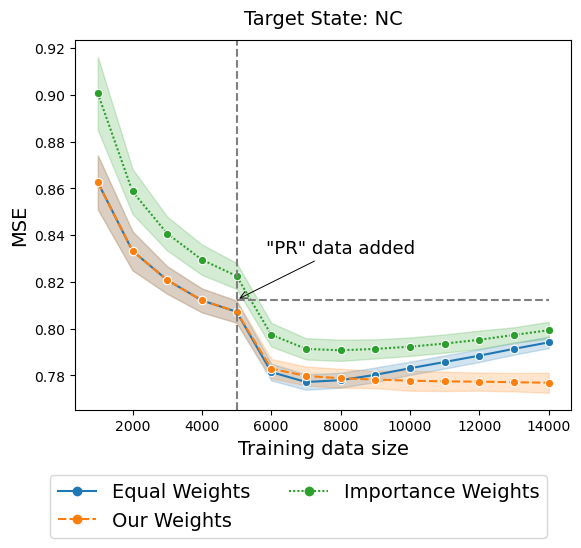
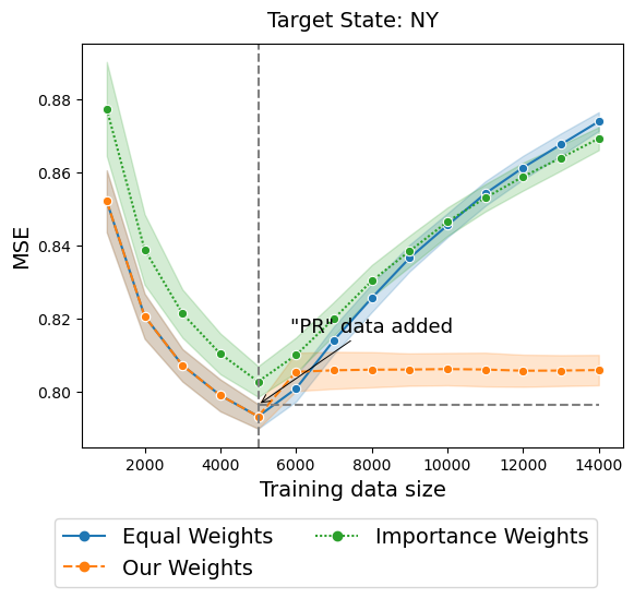
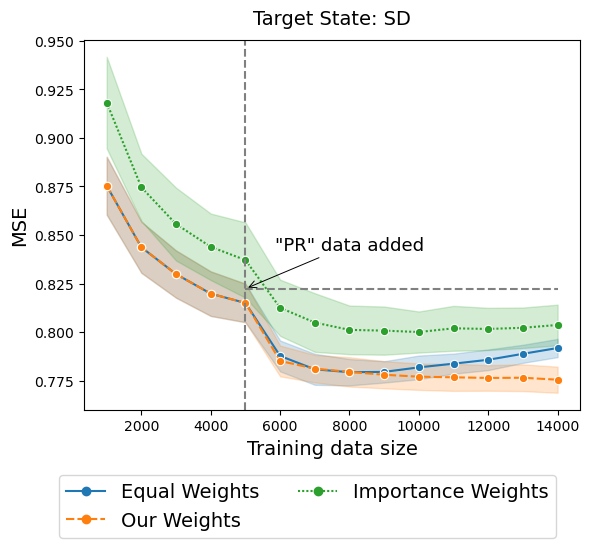
Figure 5: MSE results of the XGBoost when the training data is initially sourced from CA and then sourced from PR. The dashed vertical line indicates the point when PR data started to be added. The blue line is when samples are equally weighted, and the green line is when samples are weighted based on importance weights. The orange line is when samples receive distribution-specific weights using our proposed method.

References

- Abadie and Gardeazabal [2003] A. Abadie and J. Gardeazabal. The economic costs of conflict: A case study of the basque country. American Economic Review, 93(1):113–132, 2003.
- Abadie et al. [2007] A. Abadie, A. Diamond, and J. Hainmueller. Synthetic control methods for comparative case studies: Estimating the effect of california’s tobacco control program. Journal of the American Statistical Association, 105:493–505, 2007.
- Argyriou et al. [2007] A. Argyriou, T. Evgeniou, and M. Pontil. Multi-task feature learning. In Advances in Neural Information Processing Systems 19 (NIPS), pages 41–48, 2007.
- Athey et al. [2021] S. Athey, M. Bayati, N. Doudchenko, G. Imbens, and K. Khosravi. Matrix completion methods for causal panel data models. Journal of the American Statistical Association, pages 1–41, 2021.
- Bai [2009] J. Bai. Panel data models with interactive fixed effects. Econometrica, 77(4):1229–1279, 2009.
- Baktashmotlagh et al. [2013] M. Baktashmotlagh, M. T. Harandi, B. C. Lovell, and M. Salzmann. Unsupervised domain adaptation by domain invariant projection. Proceedings of the IEEE International Conference on Computer Vision, pages 769–776, 2013.
- Bansak et al. [2024] K. Bansak, E. Paulson, and D. Rothenhäusler. Learning under random distributional shifts. International Conference on Artificial Intelligence and Statistics, 2024.
- Ben-Tal et al. [2013] A. Ben-Tal, D. Den Hertog, A. De Waegenaere, B. Melenberg, and G. Rennen. Robust solutions of optimization problems affected by uncertain probabilities. Management Science, 59(2):341–357, 2013.
- Bodnar and Okhrin [2008] T. Bodnar and Y. Okhrin. Properties of the singular, inverse and generalized inverse partitioned wishart distributions. Journal of Multivariate Analysis, 99(10):2389–2405, 2008.
- Borenstein et al. [2009] M. Borenstein, L. V. Hedges, J. P. Higgins, and H. R. Rothstein. Introduction to Meta-Analysis. John Wiley & Sons, New York, NY, 2009.
- Cheung [2014] M. W. Cheung. Modeling dependent effect sizes with three-level meta-analyses: a structural equation modeling approach. Psychological Methods, 19(2):211–229, 2014.
- Ding et al. [2021] F. Ding, M. Hardt, J. Miller, and L. Schmidt. Retiring adult: New datasets for fair machine learning. In Advances in Neural Information Processing Systems, volume 34, pages 6478–6490, 2021.
- Doudchenko and Imbens [2016] N. Doudchenko and G. W. Imbens. Balancing, regression, difference-in-differences and synthetic control methods: A synthesis. Technical report, National Bureau of Economic Research, 2016.
- Duchi and Namkoong [2021] J. C. Duchi and H. Namkoong. Learning models with uniform performance via distributionally robust optimization. The Annals of Statistics, 49(3):1378–1406, 2021.
- Duchi et al. [2021] J. C. Duchi, P. W. Glynn, and H. Namkoong. Statistics of robust optimization: A generalized empirical likelihood approach. Mathematics of Operations Research, 46(3):946–969, 2021.
- Dudley [2018] R. M. Dudley. Real analysis and probability. CRC Press, 2018.
- Gretton et al. [2009] A. Gretton, J. Smola, M. Huang, K. Schmittfull, K. Borgwardt, and B. Schölkopf. Covariate shift by kernel mean matching. Dataset shift in machine learning, 3:131–160, 2009.
- Hartung et al. [2008] J. Hartung, G. Knapp, and B. K. Sinha. Statistical Meta-Analysis With Applications. John Wiley & Sons, New York, NY, 2008.
- Hedges et al. [2010] L. V. Hedges, E. Tipton, and M. C. Johnson. Robust variance estimation in meta-regression with dependent effect size estimates. Research Synthesis Methods, 1(1):39–65, 2010.
- Higgins et al. [2009] J. Higgins, S. G. Thompson, and D. J. Spiegelhalter. A re-evaluation of random-effects meta-analysis. Journal of the Royal Statistical Society: Series A (Statistics in Society), 172(1):137–159, 2009.
- Huber [1981] P. Huber. Robust Statistics. Wiley, New York, 1981.
- Jeong and Rothenhäusler [2023] Y. Jeong and D. Rothenhäusler. Calibrated inference: statistical inference that accounts for both sampling uncertainty and distributional uncertainty. arXiv preprint arXiv:2202.11886, 2023.
- Li et al. [2016] S. Li, S. Song, and G. Huang. Prediction reweighting for domain adaptation. IEEE Transactions on Neural Networks and Learning Systems, 28(7):1682–1695, 2016.
- Long et al. [2014] M. Long, J. Wang, G. Ding, J. Sun, and P. S. Yu. Transfer joint matching for unsupervised domain adaptation. Proceedings of the IEEE Conference on Computer Vision and Pattern Recognition, pages 1410–1417, 2014.
- Lunn et al. [2013] D. Lunn, J. Barrett, M. Sweeting, and S. Thompson. Fully bayesian hierarchical modelling in two stages, with application to meta-analysis. Journal of the Royal Statistical Society. Series C (Applied Statistics), 62(4):551–572, 2013.
- Muirhead [1982] R. J. Muirhead. Aspects of Multivariate Statistical Theory. Wiley Series in Probability and Statistics. John Wiley & Sons, Inc., 1982.
- Pan and Yang [2010] S. J. Pan and Q. Yang. A survey on transfer learning. IEEE Transactions on Knowledge and Data Engineering, 22(10):1345–1359, 2010.
- Quinonero-Candela et al. [2009] J. Quinonero-Candela, M. Sugiyama, A. Schwaighofer, and N. D. Lawrence. Dataset shift in machine learning. Mit Press, 2009.
- Rothenhäusler and Bühlmann [2023] D. Rothenhäusler and P. Bühlmann. Distributionally robust and generalizable inference. Statistical Science, 38(4):527–542, 2023.
- Schölkopf et al. [2021] B. Schölkopf, F. Locatello, S. Bauer, N. R. Ke, N. Kalchbrenner, A. Goyal, and Y. Bengio. Toward causal representation learning. Proceedings of the IEEE, 109(5):612–634, 2021.
- Shen et al. [2023] J. H. Shen, I. D. Raji, and I. Y. Chen. Mo’data mo’problems: How data composition compromises scaling properties. 2023.
- Shimodaira [2000] H. Shimodaira. Improving predictive inference under covariate shift by weighting the log-likelihood function. Journal of Statistical Planning and Inference, 90(2):227–244, 2000.
- Sugiyama et al. [2008] M. Sugiyama, S. Nakajima, H. Kashima, P. Buenau, and M. Kawanabe. Direct importance estimation with model selection and its application to covariate shift adaptation. In Advances in Neural Information Processing Systems 21 (NIPS), pages 1433–1440, 2008.
- Szegedy et al. [2014] C. Szegedy, W. Zaremba, I. Sutskever, J. Bruna, D. Erhan, I. Goodfellow, and R. Fergus. Intriguing properties of neural networks. In International Conference on Learning Representations (ICLR), 2014.
- Wood [2008] A. Wood. Methodology for dealing with duplicate study effects in a meta-analysis. Organizational Research Methods, 11:79–95, 01 2008.
- Xu [2017] Y. Xu. Generalized synthetic control method: Causal inference with interactive fixed effects models. Political Analysis, 25(1):57–76, 2017.