Casimir force within Ising chain with competing interactions

Abstract

We derive exact results for the critical Casimir force (CCF) within the one-dimensional Ising model with periodic boundary conditions (PBC’s) and long-range equivalent-neighbor ferromagnetic interactions of strength $J_{l}/N>0$ superimposed on the nearest-neighbor interactions of strength $J_{s}$ which could be either ferromagnetic ($J_{s}>0$) or antiferromagnetic ($J_{s}<0$). In the infinite system limit the model, also known as the Nagle-Kardar model, exhibits in the plane $(K_{s}=\beta J_{s},K_{l}=\beta J_{l})$ a critical line $2K_{l}=\exp{\left(-2K_{s}\right)},K_{s}>-\ln 3/4$, which ends at a tricritical point $(K_{l}=-\sqrt{3}/2,K_{s}=-\ln 3/4)$. The critical Casimir amplitudes are: $\Delta_{\rm Cas}^{\rm(cr)}=1/4$ at the critical line, and $\Delta_{\rm Cas}^{\rm(tr)}=1/3$ at the tricritical point. Quite unexpectedly, with the imposed PBC’s the CCF exhibits very unusual behavior as a function of temperature and magnetic field. It is repulsive near the critical line and tricritical point, decaying rapidly with separation from those two singular regimes fast away from them and becoming attractive, displaying in which the maximum amplitude of the attraction exceeds the maximum amplitude of repulsion. This represents a violation of the widely-accepted “boundary condition rule,” which holds that the CCF is attractive for equivalent BC’s and repulsive for conflicting BC’s independently of the actual bulk universality class of the phase transition under investigation.

Introduction: We consider the Casimir effect in a model Hamiltonian [1, 2, 3] with two competing interactions: the Ising model on a chain with “ nearest-neighbor” and with “infinitesimal equivalent-neighbor” interactions between the spins. This is known also as the Nagle-Kardar model (for reviews see [4, 5, 6]). The Hamiltonian of the model is:

$$\beta{\cal H}_{NK}(K_{l},K_{s},h)=-K_{s}\sum_{\langle i,j\rangle}^{N}S_{i}S_{j}+h\sum_{i=1}^{N}S_{i}+$$

$$-\frac{K_{l}}{N}\sum_{i,j=1}^{N}S_{i}S_{j},\;\quad K_{s},h\in\mathbb{R},\quad K_{l}\in\mathbb{R^{+}},$$ (1)

where the following notations: $K_{s}=\beta J_{s},\,K_{l}=\beta J_{l},\,h=\beta H,\,\beta=1/(k_{B}T)$, $k_{B}=1$ are used. Given the symmetry of the problem it suffices to fix $h\geq 0$.

The first two terms on the right hand side of (Casimir force within Ising chain with competing interactions) describes the Ising model with short-ranged interactions between nearest neighbors in a magnetic field $h$, on a spin chain with periodic boundary conditions and with $S_{i}=\pm 1,i=1,\cdots,N$ with interaction constant $J_{s}$. The second term is the equivalent-neighbor Ising model with infinitesimal long-ranged interaction between spins characterized by $J_{l}$. The nearest-neighbor interaction is either ferromagnetic or antiferromagnetic, i.e., $K_{s}>0$ or $K_{s}<0$, while the long-range interaction is always ferromagnetic, i.e., $K_{l}>0$. When $K_{l}<0$ there is no order at finite temperature.

This model was introduced by Baker in 1969 [1]. The seminal contributions of Nagle [2] and Kardar [3] demonstrated that the model is instructive as a means to analyze complicated phase diagrams and crossover phenomena arising from the competition between ferromagnetic and antiferromagnetic interactions. The range of subsequent work highlights the widespread interest in the properties and implications of the system [7, 8, 6, 9, 10, 11, 12, 13, 14, 15, 16, 17, 4, 5, 18, 19, 20], which has proven to be a fertile platform for the investigation of various generalizations of the competition between the antiferromagnetic and ferromagnetic interactions [21, 22, 18, 23, 24, 25, 26, 27, 19, 28]. In particular it has been shown that this simple system may well describe a number of interesting phenomena, including ensemble inequivalence [13, 15, 28], negative specific heat[13, 14, 15], ergodicity breaking [13, 14, 15], long-lived thermodynamically unstable states [13, 14], the prospect of analysis of different information estimators[21] and the cooling process of a long-range system [29].

We have discovered that the behavior of this system is interesting not only in the thermodynamic limit, in which its phase diagram is highly non-trivial, see Fig. 1, but also when the system is finite, in which case the fluctuation-induced critical Casimir force (CCF) exhibits unusually rich structure – see Figs. 2 and 3. Below we briefly explain how we obtained the results shown there.

Finite-size Gibbs free energy density (GFE) and phase diagram: In order to determine the behavior of the CCF we need to know the Gibbs free energies in the finite and infinite Ising chains with a given magnetic field $h$.

The Gibbs free energy per spin is given by

$$f_{N}[{\cal H}_{NK}(K_{l},K_{s},h)]\equiv f_{N}(K_{s},K_{l},h)=$$

$$-(\beta N)^{-1}Z_{N}(K_{s},K_{l},h),$$ (2)

where $Z_{N}(K_{s},K_{l},h)$ is the grand canonical partition function of the model. Further on, we will omit the arguments $K_{s}$, $K_{l}$ (and $h$), where this does not lead to misunderstanding.

The partition function for finite $N$ may be obtained by the well-known transfer matrix technique

$${Z_{N}(K_{s},K_{l},h)}=I^{p}_{N}\left(K_{s},K_{l},h\right)+I^{m}_{N}\left(K_{s},K_{l},h\right),$$ (3)

where

$$I^{p,m}_{N}\left(K_{s},K_{l},h\right)=\sqrt{\frac{N}{4\pi K_{l}}}\;\int_{-\infty}^{\infty}e^{-N\Psi_{p,m}(y)}dy,$$ (4)

with

$$\Psi_{p,m}(y)\left(\equiv\Psi_{p,m}(y|K_{s},K_{l},h)\right)=\frac{y^{2}}{4K_{l}}-\ln\lambda_{p,m}(h+y).$$

Here

$$\lambda_{p,m}=e^{K_{s}}\cosh(h+y)\pm\sqrt{e^{2K_{s}}\sinh^{2}(h+y)+e^{-2K_{s}}}$$ (6)

are the eigenvalues of the corresponding transfer matrix of the one-dimensional Ising model in a field $h+y$.

Since in Eq. (4) $N\gg 1$ we will calculate integrals by the Laplace method. Thus, we are interested in minimum value(s) of functions $\Psi_{k}(y),\,k=p,m$. We will see that such minima always exist at some $y_{p}^{\pm}=y_{p}^{\pm}(K_{s},K_{l},h)$ and $y_{m}^{\pm}=y_{m}^{\pm}(K_{s},K_{l},h)$. The subscript $k\,(k="p"\,\mbox{or}\,"m")$ indicates if $\lambda_{p}$ or $\lambda_{m}$ enters the corresponding function $\Psi_{k}(y)$, while superscript $l\,(l="+"\,\mbox{or}\,"-")$ is used to indicate whether the minimum lies in the $[0,\infty]$ or $[-\infty,0]$ regions of integration. From (Casimir force within Ising chain with competing interactions) one finds that $y_{k}^{\pm}=y_{k}^{\pm}(K_{l},K_{s},h)$ satisfy the equations

$$y_{k}^{\pm}=\pm\frac{2K_{l}\sinh(h+y_{k}^{\pm})}{\sqrt{\sinh^{2}(h+y_{k}^{\pm})+e^{-4K_{s}}}},\quad k=p,m.$$ (7)

We stress that $y^{\pm}_{p,m}$ do not depend on $N$. For $h=0$ these equations always have as solutions $y_{p}^{\pm}=y_{m}^{\pm}=0$.

As it will become clear later, we are interested in cases in which an expansion of the free energy in terms of the mean magnetization, $m$, starts a power of $m$ equal to $2n$ with $n\geq 1$. In such cases and for $N$ large, integrals of type (4) can be estimated by the (generalized) Laplace method [30], which states that, if on the finite interval $[a,b]\in{\mathbb{R}}$ the function $f(x)$ has a single minimum at $x_{0}$, such that $a<x_{0}<b$, $f^{(j)}(x_{0})=0$ (here $(j)$ means $j-th$ derivative with respect to $x$) with $1\leq j\leq 2n-1$, and $f^{(2n)}(x_{0})\neq 0$, with $n\geq 1$, then

$$g(N) = \int_{a}^{b}\exp[-Nf(x)]dx\simeq\Gamma\left(\frac{1}{2n}\right)\frac{[2n!]^{1/(2n)}}{n}$$

$$\times\frac{1}{N^{1/(2n)}}\frac{\exp[-Nf(x_{0})]}{\sqrt{f^{(2n)}(x_{0})}}\left(1+{\cal O}\left(N^{-1/n}\right)\right).$$

In the case of the existence of a single minimum $y^{+}_{k}$ (the choice $h>0$ implies $y_{k}^{+}$) with respect to $y$ of the functions $\Psi_{k}(y),\,k=p,m$ and where $\Psi_{k}^{(\i\i)}(y_{p,m})>0$, using the Eq.(Casimir force within Ising chain with competing interactions), with $j=n=1$, for evaluating the integrals in Eq. (3) for $N\gg 1$, we deduce for the GFE the result

$$\beta f_{N}(K_{s},K_{l},h)=\Psi_{1}(y_{p}^{+})+\frac{1}{2N}\ln\left[2K_{l}\Psi_{p}^{(\mathsf{\i}\mathsf{\i})}(y_{p}^{+})\right]-$$

$$\frac{1}{N}\ln\left\{1+\Upsilon(y_{p}^{+},y_{m}^{+})e^{\left[-N\Phi(y^{+}_{p},y^{-}_{p})\right]}\left[1+{\cal O}(N^{-1})\right]\right\},$$ (9)

where the shorthands

$$\Upsilon(y_{p}^{+},y_{m}^{+})\equiv\sqrt{\frac{\Psi_{p}^{(\mathsf{\i}\mathsf{\i})}(y_{p}^{+})}{\Psi_{m}^{(\mathsf{\i}\mathsf{\i})}(y_{m}^{+})}}\,,\,\Phi(y_{p}^{+},y_{m}^{+})\equiv\Psi_{m}(y_{m}^{+})-\Psi_{p}(y_{p}^{+})$$

are used. We recall that in deriving Eq. (Casimir force within Ising chain with competing interactions) we have assumed that $\Psi_{p}^{(\mathsf{\i}\mathsf{\i})}(y_{p}^{+})>0$ and $\Psi_{m}^{(\mathsf{\i}\mathsf{\i})}(y_{m}^{+})>0$, with $y_{\pm}$ determined from $\Psi_{p,m}^{(\mathsf{\i})}(y_{p,m})=0$. When $h\neq 0$ equations (7) have a single solution, i.e., any of the functions $\Psi_{p,m}(y)$ posses a single global minimum with respect to $y$. When $h=0$ this is not the case. As $\lambda_{p}(y)>\lambda_{m}(y)$, for al values of $y$, and so $\Psi_{p}(y)<\Psi_{m}(y)$, thus only $\Psi_{p}(y)$ will determine the bulk behavior of the system. Now, there is no difficulty in verifying that GFE in the bulk is defined as

$$\beta f_{\infty}[{\cal H}_{NK}(h)]=\inf_{m}\bigg{\{}\frac{1}{2}m^{2}-\ln[\lambda_{p}(2K_{l}m)]\bigg{\}}.$$ (10)

The value of $m$ which minimizes the expression in the curly brackets is the uniform magnetization: $m=\lim_{N\to\infty}\sum_{i}S_{i}/N$. Here the fact is used that the value of $y$ at which the function $\Psi_{p}(y)$ reaches its minimum is proportional to the magnetization per spin, i.e. $y=y_{p}^{+}=2K_{l}m$. The above results were obtained by Kardar [3].

Phase diagram: The presentation of the Gibbs free energy, Eq.(10), in terms of the power of magnetization has the form [3]

$$f_{\infty}(K_{l},K_{s},h=0)=$$

$$\inf_{m}\bigg{\{}-\ln[2\cosh(K_{s})]-K_{l}\left(2K_{l}e^{2K_{s}}-1\right)m^{2}$$

$$+(2/3)K_{l}^{4}e^{2K_{s}}\left(3e^{4K_{s}}-1\right)m^{4}+{\cal O}(m^{6})\bigg{\}}\;\;\;$$ (11)

From here we immediately conclude the existence of a line of critical points $2K_{l}=\exp{\left(-2K_{s}\right)},K_{s}>-\ln 3/4$ (then the multiplier in front of $m^{2}$ equals zero, while the one in front of $m^{4}$ is positive). If, however, $K_{s}>-\ln 3/4$ the second term will be also zero and we obtain the condition for the existence of a tricritical point. Its coordinates trivially are $(K_{l}=-\sqrt{3}/2,K_{s}=-\ln 3/4)$. The determination of the phase diagram in terms of $T$ given the values of $J_{s}$ and $J_{l}$ is, however, not so trivial. It can be achived numerically, as in Refs. [2, 3, 31, 12, 13, 21, 20, 12]. The result, which is well known, is shown in Fig. 1. Here we briefly explain how this phase diagram can be also obtained analytically in terms of the Lambert W-function[32] (also known as omega function or product logarithm; in what follows we use only its principal branch) $W_{p}(x)$ such that $W_{p}(x)\exp[W_{p}(x)]=x$. Using its properties, it is easy to show that, when $x>-1/e$, at the critical line (the red line in Fig. 1) one has $T_{c}=2J_{s}/W_{p}(x)=J_{l}[2x/W_{p}(x)]$, where $x\equiv K_{s}/K_{l}=J_{s}/J_{l}$. At this line the spontaneous magnetization critical exponent $\beta=1/2$ [2]. The green point marks the tricritical point $C$ with coordinates $\{y_{\rm TP}=2\exp[W_{p}(-\ln(3)/(2\sqrt{3}))]=2/\sqrt{3},x_{\rm TP}=-\ln(3)/(2\sqrt{3})\simeq-0.317\}$. There the spontaneous magnetization critical exponent $\beta=1/4$. The diagram also shows that a zero field first-order transition temperature (the blue line) meets the second order transition line at point $C$ that ends at $x=-0.5$. At this line three phases with the same free energy and magnetization $m=0,m=\pm m_{\rm trc}$ coexist. Above this line at zero external field the magnetization is zero, while below it there are two phases with nonzero magnetization. Since $W_{p}(\infty)\to\infty$ and $W_{p}(0)=0$, we have for the critical temperature $T_{c}(J_{s}\to 0,J_{l})=2J_{l}$ and $T_{c}(J_{s},J_{l}\to 0)=0$.

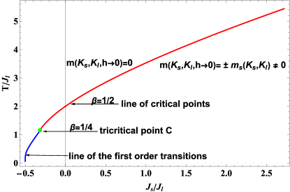
Figure 1: The phase diagram in terms of the temperature, shown as a function of $J_{s}$ and $J_{l}$. The red line $T/J_{l}=2W_{p}(x)$ represents a line of critical points, while the green point marks the tricritical point C with coordinates $\{y_{\rm TP}=2/\sqrt{3},x_{\rm TP}=-\ln(3)/(2\sqrt{3})\}$. A zero field first-order transition temperature (the blue line) meets the second order transition line at point $C$ and ends at $x=-0.5$.

Casimir force (CF): Under the assumption that the finite system of length $N$ is in contact with an infinite system characterized by the same Hamiltonian as defined in (Casimir force within Ising chain with competing interactions), for the CF we find:

$$\beta F^{\rm Cas}_{N}(K_{s},K_{l},h):=$$

$$\beta f_{\infty}(K_{s},K_{l},h)+\frac{\partial}{\partial N}\ln Z_{N}(K_{s},K_{l},h)=$$

$$\beta f_{\infty}(K_{s},K_{l},h)+\frac{1}{2N}-$$

$$\frac{\int_{-\infty}^{\infty}dy\left(\Psi_{p}(y)e^{-N\Psi_{p}(y)}+\Psi_{m}(y)e^{-N\Psi_{m}(y)}\right)}{\int_{-\infty}^{\infty}dy\left(e^{-N\Psi_{p}(y)}+e^{-N\Psi_{m}(y)}\right)},$$

where the bulk free energy per spin is given by

$$\beta f_{\infty}(K_{l},K_{s},h)$$ (13)

$$= \left\{\begin{array}[]{ll}\Psi_{p}\left(y_{p}^{+}|K_{s},K_{l},h\right),&\mbox{single minimum of}\;\Psi_{p}\\ 2\Psi_{p}\left(y_{p}^{+}=y_{p}^{-}|K_{s},K_{l},h=0\right),&\mbox{two minima of}\;\Psi_{p}.\end{array}\right.$$ (15)

Then, provided Eq. (Casimir force within Ising chain with competing interactions) is valid, for the CCF we directly obtain

$$\beta F^{\rm Cas}_{N}(K_{s},K_{l},h)=\frac{1}{N}X_{\rm Cas}(x|K_{s},K_{l},h),$$ (16)

where

$$X^{\rm Cas}_{\rm N}(x|K_{s},K_{l},h)=$$

$$-\frac{x\Upsilon(y_{p}^{+},y_{m}^{+})\exp\left[-x\right]}{1+\Phi(y_{p}^{+},y_{m}^{+})\exp\left[-x\right]}\left[1+{\cal O}(N^{-1})\right]<0,$$ (17)

with $x\equiv N\Phi(y_{p}^{+},y_{m}^{+})$. Thus, we derive that the CCF is attractive for all possible values of $K_{s},K_{l}$ and $h$. We recall that $\Psi_{p}(y_{p}^{+}|K_{s},K_{l},h)<\Psi_{m}(y_{m}^{+}|K_{s},K_{l},h)$, i.e., the force decays exponentially when $N\gg 1$; furthermore, the behavior of $y_{p}^{+}$ and $y_{m}^{+}$ as a function of $K_{s}$, $K_{l}$ and $h$ has to be determined from Eq. (7). We stress that the only dependence of the scaling function on $N$ stems from the corresponding straightforward dependence of $N$ in the scaling variable $x$. Finally, we recall that Eq. (16) is valid under the conditions which lead us to Eq. (Casimir force within Ising chain with competing interactions), namely that $\Psi_{p}^{(\mathsf{\i}\mathsf{\i})}(y_{p}^{+})>0$ and $\Psi_{m}^{(\mathsf{\i}\mathsf{\i})}(y_{m}^{+})>0$. It is easy to check, however, that at the critical line and also at the tricritical point this is no longer the case: at the line of the critical points $\Psi_{p}^{(\mathsf{\i}\mathsf{\i})}(y_{p}^{+}=0)=0$, while $\Psi_{m}^{(\mathsf{\i}\mathsf{\i})}(y_{m}^{+}=0)=1/K_{l}>0$. Thus, Eq. (Casimir force within Ising chain with competing interactions) and Eq. (Casimir force within Ising chain with competing interactions) are no longer valid. Furthermore, one obtains $\Psi_{p}^{(\mathsf{\i}\mathsf{\i}\mathsf{\i})}(y_{+})=0$, while $\Psi_{p}^{(\mathsf{\i}\mathsf{v})}(y^{+}_{p}=0)=e^{2K_{s}}\left(3e^{4K_{s}}-1\right)>0$ if the system is not positioned at the tricritical point. However, $\Psi_{p}^{(\mathsf{\i}\mathsf{v})}(y_{p}^{+}=0)=0$ at this point, while $\Psi_{p}^{(\mathsf{v}\mathsf{\i})}(y_{p}^{+}=0|K_{s}=-\ln 3/4,K_{l}=\sqrt{3}/2,h=0)=4/\sqrt{3}>0$. These facts lead to the following results:

i) The Casimir force at the critical line is:

$$\beta F^{\rm Cas}_{\rm N}(K_{s},K_{l}=e^{-2K_{s}}/2,h=0)$$

$$= \frac{1}{N}\left\{\frac{1}{4}+{\cal O}\left[N^{-1/4}\exp[-2N\tanh^{-1}\left(e^{-2K_{s}}\right)]\right]\right\}.$$

ii) At the tricritical point the following expression for the tricritical Casimir force (TCF) holds:

$$\beta F^{\rm Cas}_{\rm N}(K_{s}=-\ln 3/4,K_{l}=\sqrt{3}/2,h=0)$$

$$= \frac{1}{N}\left\{\frac{1}{3}+{\cal O}\left[N^{-1/3}\exp\left[-2N\coth^{-1}\left(\sqrt{3}\right)\right]\right]\right\}.$$

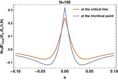
Figure 2: The behavior of the CCF pertinent to NK model as a function of $h$ for different fixed values of $K_{s}$ and $K_{l}$ with $N=100$. The red line corresponds to $K_{s}=0,K_{l}=0.5$, while the blue line corresponds to the tricritical point which emerges in the phase diagram at coordinate $K_{s}=-\ln 3/4,K_{l}=\sqrt{3}/2$ obtained from the conditions: the multipliers in front of $m^{2}$ and $m^{4}$ equal zero, see Eq.(Casimir force within Ising chain with competing interactions). The results are in a full agreement with the derived exact results - see Eq. (Casimir force within Ising chain with competing interactions) and Eq. (Casimir force within Ising chain with competing interactions).

iii) Close above ($+$), or below ($-$) the critical line:

$$\beta F^{\rm Cas}_{\rm N}(K_{s},K_{l},h=0,N)=-\frac{1}{N}\sqrt{\frac{\pm\left[2K_{l}e^{2K_{s}}-1\right]N^{1/\nu_{\rm MF}}}{2K_{l}e^{2K_{s}}+1}}$$

$$\times\xi_{I}(K_{s})^{-1}\exp\left[-N/\xi_{I}(K_{s})\right]\left[1+{\cal O}(N^{-1})\right].$$ (20)

Here $\nu_{\rm MF}=1/2$ and

$$\xi_{I}(K_{s},h=0)=\ln[\lambda_{p}/\lambda_{m}]^{-1}=-1/\ln[\tanh(K_{s})]$$ (21)

is the correlation length (for $K_{s}\geq 0$ one has $\ln(\tanh(K_{s}))<0$) of the one-dimensional Ising model for $h=0$ [33]. Thus, according to Eq. (Casimir force within Ising chain with competing interactions), the CCF close above or below the critical line is attractive and decays exponentially with $N\gg 1$. Let us note, however, that in the current problem we consider $K_{s}=O(1)$ along the line of critical points, i.e., $\xi_{I}={\cal O}(1)$. Thus, in such a case $\left[2K_{l}e^{2K_{s}}-1\right]N^{1/\nu_{\rm MF}}$ plays the role of a scaling variable.

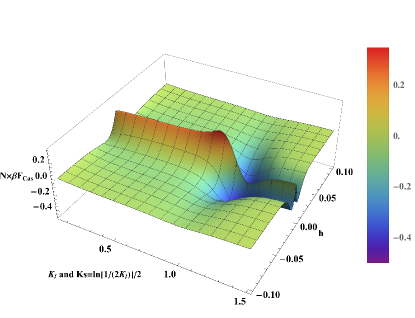
Figure 3: The 3D visualization of the behavior of the CCF as a function of $h$ for different fixed values of $K_{s}$ and $K_{l}$ with $N=100$. Here $K_{l}\in(0,1.5]$ while $K_{s}=\ln\left[1/(2K_{l})\right]/2$ (i.e. on the line of the critical points). The results are in a full agreement with the derived exact results - see Eq. (Casimir force within Ising chain with competing interactions) and Eq. (Casimir force within Ising chain with competing interactions). As we see — despite the boundary conditions being periodic, in the framework of the NK model the CCF can be both repulsive and attractive, depending on the values of $K_{l},K_{s}$ and $h$. Obviously, the force is symmetric with respect to $h=0$ as a function of $h$.

iv) The case of nonzero external field, i.e., $h\neq 0$.

In this case the result for the CCF is given by Eq. (16) and Eq. (Casimir force within Ising chain with competing interactions). The force is attractive.

The general behavior of the CCF is numerically obtained and visualized in Figs. 2 and 3. We observe that the analytical expressions presented above confirm our analytical findings.

Conclusion: In the available literature on CCF’s the following “boundary conditions rule” is widely accepted: in the whole range of temperatures, independently of the actual bulk universality class of the phase transition, the arising CCF is attractive for equal (symmetric) BC’s [say, $(+,+)$, or $(0,0)$] and repulsive for unequal (asymmetric) BC’s [say, antiperiodic or $(+,-)$] [34, 35, 36]. Indeed, the above statement is not a proven theorem, but an empirical finding that has been tested on a large number of models[35]. As we see, for the NK model under periodic boundary conditions this is not the case.

Our main results are:

- We have derived a closed-form analytic expression for the critical temperature of the second-order phase transition, $T_{c}(J_{s},J_{l})$, in terms of the Lambert W-function. This expression allows for the clarification of the behavior of the critical temperature as a function simultaneously of the two interaction constants $K_{s}$ and $K_{l}$ of the model (see Fig. 1).

- We show that the CCF is repulsive at the critical line and at the tricritical point, in spite of the applied periodic boundary conditions. The behavior of the tricritical Casimir force (TCF) is presented and compared with the standard CCF in Fig. 2. The exact Casimir amplitudes are: $\Delta_{\rm Cas}^{\rm(cr)}=1/4$ at the critical line, and $\Delta_{\rm Cas}^{\rm(tr)}=1/3$ at the tricritical point.

- Close to the critical line and the tricritical point the CF decays rapidly with distance away from them in the (temperature–field plane) - see Eq. (Casimir force within Ising chain with competing interactions). For $h\neq 0$ the CF is attractive - see Eq. (Casimir force within Ising chain with competing interactions).

In essence, our main results are summarized, in form of 3-d behavior of the CCF, as a function of $h$ for different fixed values of $K_{s}$ and $K_{l}$, in Fig. 3. While the plot is in agreement with all analytical results stated above, we observe regions in which it is magnitude of the attraction exceeds that of its repulsion, when it is repulsive. Currently, we do not have analytical results for these regions.

Finally, we stress that the mechanism for changing the sign of the CCF is highly non-trivial and may not depend solely on whether the imposed boundary conditions are symmetrical or not. The beyond-mean-field model considered here shows that the ‘boundary condition rule’ is an incomplete statement and the presence of the competing interactions also matters. We note that a CCF with behavior that is repulsive or attractive, depending on the values of $T$ and $h$ has been also observed in the case of a ferromagnetic Ising ring with a competitive single antiferromagnetic bond [37].

Acknowledgments: The authors thank Prof. M. Kardar for suggesting the problem and for a valuable discussion on the topic.

The partial financial support via Grant No KP-06-H72/5 of Bulgarian NSF is gratefully acknowledged.

References

- Baker [1963] G. A. Baker, Phys. Rev. 130, 1406 (1963), ISSN 0031-899X, URL <GotoISI>://WOS:A19631495C00003.
- Nagle [1970] J. F. Nagle, Phys. Rev. A 2, 2124 (1970), URL <GotoISI>://WOS:A1970I120600075.
- Kardar [1983] M. Kardar, Phys. Rev. B 28, 244 (1983), ISSN 0163-1829, URL <GotoISI>://WOS:A1983QY61100026.
- Patelli and Ruffo [2013] A. Patelli and S. Ruffo, Rivista Di Matematica Della Universita Di Parma 4, 345 (2013), ISSN 0035-6298, URL <GotoISI>://WOS:000214377000004.
- Campa et al. [2014] A. Campa, T. Dauxois, D. Fanelli, and S. Ruffo, Physics of long-range interacting systems (Oxford University Press, Oxford, 2014), first edition. ed., ISBN 9780199581931 (hbk.) 0199581932 (hbk.).
- Gupta and Ruffo [2017] S. Gupta and S. Ruffo, Int. J. Mod. Phys. A 32 (2017), ISSN 0217-751X, URL <GotoISI>://WOS:000398867000008.
- Hoye [1972] J. S. Hoye, Physical Review B 6, 4261 (1972), URL <GotoISI>://WOS:A1972O059000021.
- Kaufman and Kahana [1988a] M. Kaufman and M. Kahana, Phys. Rev. B 37, 7638 (1988a), ISSN 0163-1829, URL <GotoISI>://WOS:A1988N304600058.
- Vieira and Goncalves [1995] A. Vieira and L. Goncalves, Condens. Matter Phys. pp. 210–225 (1995).
- Paladin et al. [1994] G. Paladin, M. Pasquini, and M. Serva, Journal De Physique I 4, 1597 (1994), ISSN 1155-4304, URL <GotoISI>://WOS:A1994PP72400004.
- Vieira and Goncalves [1999] A. P. Vieira and L. L. Goncalves, J. Magn. Magn. Mater. 192, 177 (1999), ISSN 0304-8853, URL <GotoISI>://WOS:000078289900022.
- Boukheddaden et al. [2000] K. Boukheddaden, J. Linares, H. Spiering, and F. Varret, Eur. Phys. J. B 15, 317 (2000), ISSN 1434-6028, URL <GotoISI>://WOS:000087440800016.
- Mukamel et al. [2005] D. Mukamel, S. Ruffo, and N. Schreiber, Phys. Rev. Lett. 95 (2005), ISSN 0031-9007, URL <GotoISI>://WOS:000233826100012.
- Mukamel [2009] D. Mukamel, arXiv:0905.1457 [cond-mat.stat-mech] (2009), URL https://doi.org/10.48550/arXiv.0905.1457.
- Campa et al. [2009] A. Campa, T. Dauxois, and S. Ruffo, Phys. Rep. 480, 57 (2009), ISSN 0370-1573, URL <GotoISI>://WOS:000269989400001.
- Bouchet et al. [2010] F. Bouchet, S. Gupta, and D. Mukamel, Physica A 389, 4389 (2010), ISSN 0378-4371, URL <GotoISI>://WOS:000281997300010.
- Ostilli [2012] M. Ostilli, Epl 97 (2012), ISSN 0295-5075, URL <GotoISI>://WOS:000301952600008.
- Salmon et al. [2015] O. D. R. Salmon, J. R. de Sousa, and M. A. Neto, Phys. Rev. E 92 (2015), ISSN 1539-3755, URL <GotoISI>://WOS:000361310100002.
- Kardar and Kaufman [1983] M. Kardar and M. Kaufman, Phys. Rev. Lett. 51, 1210 (1983), URL https://link.aps.org/doi/10.1103/PhysRevLett.51.1210.
- Kaufman and Kahana [1988b] M. Kaufman and M. Kahana, Phys. Rev. B 37, 7638 (1988b).
- Cohen et al. [2015] O. Cohen, V. Rittenberg, and T. Sadhu, J. Phys. A 48 (2015), ISSN 1751-8113, URL <GotoISI>://WOS:000347848500003.
- Li and Hou [2022a] Z. X. Li and J. X. Hou, Mod. Phys. Lett. B 36 (2022a), ISSN 0217-9849, URL <GotoISI>://WOS:000846687500008.
- Campa et al. [2019] A. Campa, G. Gori, V. Hovhannisyan, S. Ruffo, and A. Trombettoni, J. Phys. A 52 (2019), ISSN 1751-8113, URL <GotoISI>://WOS:000478799100002.
- Yang and Hou [2022] J. T. Yang and J. X. Hou, Eur. Phys. J. B 95 (2022), ISSN 1434-6028, URL <GotoISI>://WOS:000882380900001.
- Salmon et al. [2016] O. D. R. Salmon, J. R. de Sousa, M. A. Neto, I. T. Padilha, J. R. V. Azevedo, and F. D. Neto, Physica a-Statistical Mechanics and Its Applications 464, 103 (2016), ISSN 0378-4371, URL <GotoISI>://WOS:000384382600009.
- Yao and Hou [2021] Y. C. Yao and J. X. Hou, Int. J. Theor. Phys. 60, 968 (2021), ISSN 0020-7748, URL <GotoISI>://WOS:000610019700001.
- Campa et al. [2021] A. Campa, G. Gori, V. Hovhannisyan, S. Ruffo, and A. Trombettoni, J. Stat. Phys. 184 (2021), ISSN 0022-4715, URL <GotoISI>://WOS:000692356300002.
- Yang et al. [2024] J.-T. Yang, Q.-Y. Tang, and J.-X. Hou, Chinese Journal of Physics 89, 1325 (2024), ISSN 0577-9073.
- Li and Hou [2022b] Z. X. Li and J. X. Hou, Mod. Phys. Lett. B 36 (2022b), ISSN 0217-9849, URL <GotoISI>://WOS:000846687500008.
- Fedoryuk [1987] M. V. Fedoryuk, Asymptotic: Integrals and Series (in Russian) (Nauka, Moscow, 1987), in Russian.
- Kislinsky and Yukalov [1988] V. B. Kislinsky and V. I. Yukalov, Journal of Physics a-Mathematical and General 21, 227 (1988), ISSN 0305-4470, URL <GotoISI>://WOS:A1988L660000027.
- Olver et al. [2010] F. W. J. Olver, N. I. of Standards, and T. (U.S.), NIST handbook of mathematical functions (Cambridge University Press : NIST, Cambridge ; New York, 2010), ISBN 9780521192255 (hbk.) 0521192250 (hbk.) 9780521140638 (pbk.) 0521140633 (pbk.).
- Baxter [1982] R. J. Baxter, Exactly Solved Models in Statistical Mechanics (Academic, London, 1982).
- Rafaïet al. [2007] S. Rafaï, D. Bonn, and J. Meunier, 386, 31 (2007), URL https://doi.org/10.1016/j.physa.2007.07.072.
- Dantchev and Dietrich [2023] D. Dantchev and S. Dietrich, Phys. Rep. 1005, 1 (2023), ISSN 0370-1573, URL https://www.sciencedirect.com/science/article/pii/S0370157322004070.
- Gambassi and Dietrich [2024] A. Gambassi and S. Dietrich, Soft Matter (2024), ISSN 1744-6848.
- Dantchev and Tonchev [2024] D. Dantchev and N. Tonchev, arXiv:2403.17109 [cond-mat.stat-mech] (2024), eprint 2403.17109.