Relational Lorentzian Asymptotically Safe Quantum Gravity:
Showcase model
¹ Inst. for Quantum Gravity, FAU Erlangen – Nürnberg,
Staudtstr. 7, 91058 Erlangen, Germany

Abstract

In a recent contribution we identified possible points of contact between the asymptotically safe and canonical approach to quantum gravity. The idea is to start from the reduced phase space (often called relational) formulation of canonical quantum gravity which provides a reduced (or physical) Hamiltonian for the true (observable) degrees of freedom. The resulting reduced phase space is then canonically quantised and one can construct the generating functional of time ordered Wightman (i.e. Feynman) or Schwinger distributions respectively from the corresponding time translation unitary group or contraction semigroup respectively as a path integral. For the unitary choice that path integral can be rewritten in terms of the Lorentzian Einstein Hilbert action plus observable matter action and a ghost action. The ghost action depends on the Hilbert space representation chosen for the canonical quantisation and a reduction term that encodes the reduction of the full phase space to the phase space of observavbles. This path integral can then be treated with the methods of asymptically safe quantum gravity in its Lorentzian version.

We also exemplified the procedure using a concrete, minimalistic example namely Einstein-Klein-Gordon theory with as many neutral and massless scalar fields as there are spacetime dimensions. However, no explicit calculations were performed. In this paper we fill in the missing steps. Particular care is needed due to the necessary switch to Lorentzian signature which has strong impact on the convergence of “heat” kernel time integrals in the heat kernel expansion of the trace involved in the Wetterich equation and which requires different cut-off functions than in the Euclidian version. As usual we truncate at relatively low order and derive and solve the resulting flow equations in that approximation.

1 Introduction

The asymptotically safe quantum gravity (ASQG) [2] and canonical quantum gravity [3] programmes are both non-perturbative approaches with the common goal to synthesise Quantum Field Theory (QFT) and General Relativity (GR). However, there appear to be profound differences between the two at a very deep level:
1. While ASQG uses mostly Euclidian signature, CQG uses exclusively Lorentzian signature.
2. While ASQG employs background dependent methods, CQG is manifestly background independent.
3. While ASQG relies on truncations of the exact renormalisation flow (Wetterich) equations, no truncations are performed in CQG.
These differences are so drastic that very little contact between the two programmes has been established so far.

In a recent contribution [4] we have advertised the point of view that these differences are possibly not as unsurmountable as they appear to be. First of all, there are also Lorentzian versions of the Wetterich equation which were applied to matter quantum fields and gravity [5, 6, 7, 8, 9]. Next, the apparent background dependence of ASQG is mostly a misunderstanding if one uses the background techniques of ASQG properly. Namely, the so called background field method [10] was invented for QFT without gravity as a tool to compute the effective action (i.e. the generating functional of connected, 1-PI, time ordered distributions) which by itself is of course background independent and which results from the background dependent object by equating the background field with the current on which the background independent effective action depends. In order that this works, one must use unspecified background fields which are not subject to any particular restrictions such as symmetries. Finally, the truncations performed in ASQG are not required in principle but in practice in the sense of an approximation scheme which, to the best of our knowledge, is the case for all known renormalisation procedures. In view of the fact that also in CQG renomalisation is necessary [11], not in order to tame quantum divergences but to fix quantum ambiguities, approximation methods will be necessary in CQG as well. The challenge is to show mathematically that truncations are really approximations, i.e. that there is some form of error control or convergence which to the best of our knowledge has not been established yet.

Accordingly it is well motivated to have a fresh look at both programmes and try to bring them into closer contact (see [12, 13] for previous attempts). In [4] we have tried to to give a compact description of both programmes useful for researchers from both communities in order to overcome differences of language. For ASQG practitioners we have laid out the basics of reduced phase space quantisation, relational observables, Hilbert space representations of the associated Weyl algebras supporting given Hamiltonian operators and the passage from the operator to the path integral formulation in particular in the presence of gauge symmetries. For CQG practitioners we have reviewed the background field method in the presence of gauge symmetries, the effective (average) action, the Wetterich equation [14, 15], heat kernel techniques [16] for both signatures and truncation methods.

In application to GR one finds the following general features independent of the matter content of the system:
A. First, if the goal is to write the path integral in terms of the Einstein Hilbert action plus matter and further terms, then Lorentzian signature is selected. If one is content to write the theory just as some sort of path integral, then the Euclidian version is also possible for the generating functional of Schwinger functions which are generated by the given Hamiltonian via Osterwalder-Schrader reconstruction [17].
B. Next, the path integral “measure” deviates from the “Lebesgue measure” of the spacetime metric by several functions which depend on the chosen Hilbert space representation of the Weyl algebra, the determinant of the deWitt metric and as a result of the splitting of the metric into ADM variables. Some of these factors, but not all, can be absorbed into a ghost action which is related to the usual ghost action that results from the Fadeev Popov determinant as a result of gauge fixing the metric to some, say de Donder, gauge.
C. The Einstein Hilbert plus observable matter action is corrected by a “reduction” action which plays a role similar to a gauge fixing action but here is rather a fingerprint of how the gauge degrees of freedom have been absorbed into the observables of the theory in a way similar to the Higgs mechanism. Accordingly, the true degrees of freedom contain $d(d+1)/2-d$ rather than $d(d+1)/2-2d$ observable gravity polarisations in $d$ spacetime dimensions as they have “eaten” $n$ scalar fields and have become “Goldstone” bosons.
D. Furthermore, the generating functional of Feynman distributions contains a current only for the observable $d(d+1)/2-d$ gravity polarisations, not for all of them. For reasons of better comparability with the existing ASQG literature one can by hand augment the current by additional terms to include also the unphysical $d$ gravity polarisations (which are integrated out in the correct non-augmented version by performing the lapse and shift integral) but one has to be careful in the interpretation of the resulting effective action: Its restriction to the observable part of the current is not the observable effective action that one is interested in, rather the two are related by a twisted combination of Legendre transforms and restriction maps.
E. Finally, one has to add the cut-off action to define the effective average action. This, like the Einstein-Hilbert action comes with a factor of $i$ in the exponent in its Lorenzian version and requires a different type of cut-off functions than in the Euclidian signature case.

In [4] we have exemplified these general techniques for GR coupled to a very simple matter content as a showcase model, namely the Einstein Hilbert action in $d$ spacetime dimensions minimally coupled to $d$ neutral, massless Klein Gordon fields studied in [18] from a CQG perspective, in order to have a concrete example in mind. However, we only prepared this showcase model to make it ready for a ASQG treatment, the analysis itself was not carried out. This is the subject of the present paper. Thus we will write the concrete Wetterich equation for this model and derive the resulting flow equations in the lowest order truncation for the three coupling parameters on which this model depends. We show that there exist cut-off functions for which the required “heat” kernel time integrals are finite. The Lorentzian heat kernel traces can otherwise be performed almost signature independently. In particular the so-called “non-minimal” term techniques [19] can be copied literally. In this exploratory paper we ignore the effect of the ghost integral as a first step. This shows that the ASQG and CQG formalisms can be brought into contact, not only in principle but also very concretely.

The architecture of this contribution is as follows:

In section 2 we review the bare bones from [4] necessary to be able to carry out the calculations of the present paper.

Section 3 contains the main results of this paper. We formulate the non-perturbative Wetterich equation for this model and then truncate it to first few terms. We compute the required heat kernel traces in that approximation paying attention to non-minimal terms. Next we perform the heat kernel time integrals with respect to a new kind of cut-off that has to have different analytic properties than in the Euclidian signature case as what is relevant here are not Laplace but Fourier transforms. As shown in [4] (appendix C) these cut-off functions can also be used in the Euclidian regime. Finally we compute the flow equations for the three parameter space of dimensionless couplings of the present model and study their solutions and fixed points. We are particularly interested in the $k\to 0$ limit of the dimensionful couplings which defines the effective action of actual interest. A new feature of the Lorentzian flow is that at $k\not=0$ the couplings become generically complex valued. However, only the $k=0$ values of the couplings have physical meaning and thus the physically relevant or admissible trajectories are restricted to those for which all dimensionful couplings are real valued at $k=0$.

In section 4 we summarise and conclude.

2 The model and Lorentzian tools

The purpose of this section is to extract from [4] the ingredients necessary in order to jump right away into the the ASQG treatment of the next section.

2.1 CQG derivation

The starting point is the classical action of the model

$$S=G_{N}^{-1}\;\int_{M}\;d^{d}x\;\sqrt{-\det(g)}\;[R[g]-2\Lambda-\frac{G_{N}}{2}S_{IJ}\;g^{\mu\nu}\;\phi^{I}_{,\mu}\;\phi^{J}_{,\nu}]$$ (2.1)

where $M$ is a d-dimensional manifold, necessarily diffeomorphic to $\mathbb{R}\times\sigma$ where $\sigma$ is a $(d-1)$ dimensional manifold when $g$ is metric of Lorentzian signature and $(M,g)$ is a globally hyperbolic spacetime which is a necessary assumption in CQG [20]. To avoid discussions about boundary terms we assume that $\sigma$ is compact without boundary, say a $d-$torus. Furthermore, $R$ is the Ricci scalar, $G_{N}$ is Newton’s constant and $\Lambda$ is the cosmological constant. The matter content consists of $d$ neutral scalar fields $\phi^{I},\;I=0,..,d-1$ which minimally couple to to the metric via a constant, real valued and positive definite matrix $S$.

The Legendre transform of the Lagrangian displayed in (2.1) is singular and leads to $2d$ first class constraints. There is a set of $d$ primary constraints $C^{1}_{\mu}$ which state that in the ADM formulation of (2.1) the momenta conjugate to lapse and shift functions are identically zero and these induce $d$ secondary constraints $C^{2}_{\mu}$ known as $d-1$ spatial diffeomorphism constraints and one Hamiltonian constraint [21]. For the above model the unreduced phase space consists of the canonical pairs $(P_{\mu},N^{\mu}),(p^{ab},q_{ab}),(\pi_{I},\phi^{I})$ with $\mu=0,..,d-1,\;a=1,..,d-1$ where $N^{0},N^{a}$ are lapse and shift functions respectively and $q_{ab}$ is the metric on $\sigma$. The other variables denote the conjugate momenta. In the reduced phase space approach one imposes $2d$ gauge fixing conditions, on the configuration variables and solves the constraints for the $2d$ conjugate momenta. A convenient set of gauge conditions is that

$$G_{2}^{I}:=\phi^{I}-k^{I}=0,\;G_{1}^{\mu}:=N^{\mu}-c^{\mu}=0$$ (2.2)

where $k^{I},c^{\mu}$ are functions on $M$ independent of the phase space variables subject to the condition that $\det(\partial k/\partial x)\not=0$. Accordingly we solve the constraints $C^{2}_{\mu}=0,C^{1}_{\mu}=P_{\mu}=0$ for $\pi_{I},P_{\mu}$ which is trivial for $P_{\mu}$. The secondary constraints can be solved algebraically for $\pi_{I}:=\pi^{\ast}_{I}$ [4]. In this way the gauge degrees of freedom are identified as $(N^{\mu},\phi^{I}),(P_{\mu},\pi_{I})$ while the true degrees of freedom are $(q_{ab},p^{ab})$.

To obtain the reduced Hamiltonian we note that the so called primary Hamiltonian for generally covariant systems is a linear combination of constraints, in this case

$$H_{{\sf primary}}=\int\;d^{3}x\;[v^{\mu}\;C^{1}_{\mu}+N^{\mu}\;C^{2}_{\mu}]$$ (2.3)

where $C_{0},C_{a}$ are the Hamiltonian and spatial diffeomorphism constraints. Here $v^{\mu}$ are the velocities with respect to which the Legendre transform is singular. The gauge stability condition imposes that the gauge fixing condition be preserved in time

$$\dot{G}_{2}^{I}=\partial_{t}G_{2}^{I}+\{H_{{\sf primary}},G_{2}^{I}\}=\{H_{{\sf primary}},G_{2}^{I}\}-\dot{k}^{I}=0,\;\dot{G}_{1}^{\mu}=\partial_{t}G_{1}^{I}+\{H_{{\sf primary}},G_{2}^{I}\}=v^{\mu}-\dot{c}^{\mu}=0$$ (2.4)

which can be solved for $N^{\mu}:=N^{\mu}_{\ast}$ and $v^{\mu}:=v^{\mu}_{\ast}=\dot{c}^{\mu}=\dot{N}^{\mu}_{\ast}$. The reduced Hamiltonian is defined to be that function of the true degrees of freedom only which generates the same equations of motion as the primary Hamiltonian when we restrict to the reduced phase space i.e.

$$\{H,F\}=\{H_{{\sf primary}},F\}_{\ast}$$ (2.5)

where the subscript $\ast$ instructs to evaluate the Poisson bracket taken on the unreduced phase space and then freeze it to $P_{\mu}^{\ast},\pi_{I}^{\ast},N^{\mu}_{\ast},\phi^{I}_{\ast},v^{\mu}_{\ast}$. Here $F$ is a function of $(q,p)$ only. The explicit expression for H is given in [4]. It is conservative, i.e. not explicitly time dependent iff $\kappa^{I}_{\mu}:=\partial k^{I}/\partial x^{\mu}$ is time $x^{0}$ independent. This is the simplest choice of gauge also adopted in [4] and while not necessary simplies the formulae.

Equipped with the reduced phase space coordinatised by $(q,p)$, the reduced Hamiltonian and a preferred time direction $x^{0}$, we can now quantise the system by imposing canonical commutation and $\ast$ relations in the usual way which gives rise to a Weyl algebra $\mathfrak{A}$ for which we can pick Hilbert space representations. The cyclic representations correspond to states $\omega$ [22] with respect to which we can compute time ordered correlation functions (Feynman distributions) which can be analytically continued in time due to the conservative nature of the Hamiltonian (Schwinger distributions). These distributions are obtained from a generating functional $Z_{s}[f]$ which depends on currents $f^{ab}$ for $q_{ab}$ where $s=0,1$ corresponds to Euclidian and Lorentzian time respectively.

These generating functionals can be cast into a formal path integral over the phase space spactime fields $(q,p)$ by the usual methods and assumptions familiar from ordinary QFT and depend on the Euclidian or Lorentzian phase space action induced by H respectively. Specifically

$$Z_{s}[f]=\int\;[dq\;dp]\;J_{\omega}[q]\;e^{-\int\;dx^{0}\;(i\;<p,\dot{q}>+(-i)^{s}\;H[p,q])}\;e^{i^{s}\;\int\;dx^{0}\;<f,q>}$$ (2.6)

where $<.,.>$ is the inner product on $\otimes^{d(d-1)/2}\;L_{2}(\sigma,d^{d-1}x)$ between symmetric twice contravariant tensor densities of weight one and twice symmetric covariant tensors and $J_{\omega}[q]$ is a functional that depends on the chosen state $\omega$ on $\mathfrak{A}$ [4].

One now would like to perform the momentum integrals. This is difficult because $H$ involves a square root that originates from solving the constraints $C_{\mu}$ for the momenta $\pi_{I}$ on which they depend quadratically. Thus (2.6) is not at all a simple Gaussian integral in $p$. In [4] two possibilities for getting rid off the square root were presented. The first method introduces a single auxiliary field $\lambda$ and is inspired by the observation that the critical point value of the function $\lambda\mapsto[\lambda\;h+\lambda^{-1}]/2$ is given by $\sqrt{h}$ so that in a saddle point approximation of the $\lambda$ integral one obtains the square root. In [4] the exact version of this saddle point argument is presented. It has the advantage that it works in principle for both signatures but it has the disadvantage of being spatially non-local involving the solution of PDE’s that arise when integrating out $p$. We hope to come back to this method for the present model in a future publication. Alternatively, there exists also scalar matter which avoids the square root from the outset [23] which would also be interesting to study.

The second method follows the well known procedure [24] for unfolding a reduced phase space path integral to the unreduced phase space by introducing $\delta$ distributions for $G_{2}^{\mu},C^{2}_{\mu}$ and the determinant of the Dirac matrix $\Delta:=\{C^{2},G_{2}\}$ which is very similar to the Lagrangian Fadeev-Popov method. Thus the path integral is extended to an integration also over $\phi^{I},\pi_{I},N^{\mu}$ where the integral over $N^{\mu}$ yields $\delta[C^{2}]$ and we keep $\delta[G^{2}]\;\det(\Delta)$ untouched. This enables to replace $H[q,p]$ by $-<\pi,\dot{\phi}>$ in (2.6) because $H=-<\pi_{\ast},\dot{k}>$ at the price to augment the exponent by $-i\;<N,C^{2}>$ which installs the $\delta[C^{2}]$ distribution. We now see that for $s=0$ we run into trouble: The terms $<p,\dot{q}>,<\pi,\cdot{\phi}>$ come with a relative factor of $i$. Then carrying out the now Gaussian integrals over $\pi,p$ turns the exponent into the Einstein Hilbert action for complex GR plus corrections.

This forces us to work with $s=1$ from now on. The Gaussian integrals over $p,\pi$ can be performed which introduces a measure factor depending on $q,N$. We also carry out the integral over $\phi$ via $\delta[G_{2}]$ which replaces $\phi^{I}_{,\mu}$ by $k^{I}_{,\mu}=\kappa^{I}_{\mu}$. Then the integral only involves $q_{ab},N^{\mu}$. By switching integration variables to $g_{\mu\nu}$ using the ADM relations $g_{00}=-N^{2}+q_{ab}N^{a}N^{b},\;g_{0a}=q_{ab}N^{b},\;g_{ab}=q_{ab}$ we can write $[dq\;dN]=[dg]\;I[q,N]$ with the corresponding Jacobean $I[q,N]$ so that we end up with a functional integral over Lorentzian signature spacetime metrics $g$, specifically

$$Z_{1}[f]=\int\;[dg]\;J_{\omega}[g]\;e^{-iS_{1}[g]\;}\;e^{i\int_{M}\;d^{d}x\;f^{ab}q_{ab}},\;\;S_{1}[g]=\frac{1}{G_{N}}\int_{M}\;d^{d}x\sqrt{-\det(g)}[R[g]-2\Lambda-\frac{G_{N}}{2}g^{\mu\nu}\;S_{IJ}\;\;k^{I}_{,\mu}\;k^{J}_{,\nu}]$$ (2.7)

where we have collected all measure factors that deviate from the exponential of the displayed action into the function $J_{\omega}[g]$ [4] written in terms of $g$ rather than $q,N$ which again depends on the state $\omega$. It can be written in terms of a functional determinant $J_{\omega}=\det(K_{\omega})$, hence the second factor may be replaced by a ghost integral if wanted [4]

$$J_{\omega}[g]=|\int[d\rho\;d\eta]\;e^{-i\int\;d^{d}x\;\eta^{\mu}\;[K_{\omega}]_{\mu}^{I}(g)\;\rho_{I}}|$$ (2.8)

where $K_{\omega}$ is the ghost matrix [4] (we consider only the case $\kappa^{I}_{\mu}=$const. and $\kappa^{I}_{0}=\kappa_{0}\delta^{I}_{0}$)

$$[K_{\omega}]_{\mu}^{I}(g) = f_{\omega}(g)\{\frac{\delta_{\mu}^{0}}{N}[\kappa^{I}_{0}-N^{a}\kappa^{I}_{a}]+\delta_{\mu}^{a}\kappa_{a}^{I}\},\;$$

$$f_{\omega}(g) = |-\det(g)|^{2/d-(d+1)/8}\;|\det(q)|^{2/d+(d+1)/4}\;\exp(h_{\omega}/d)$$

$$h_{\omega}(x^{0},\vec{x}) = [\delta(x^{0},\infty)+\delta(x^{0},-\infty)]\;I_{\omega}(x^{0},\vec{x}),\;\Omega_{\omega}[q(x^{0})]=:\exp(\int\;d^{d-1}x\;I_{\omega}(x^{0},\vec{x}))$$ (2.9)

and $q,N$ are to be expressed in terms of $g$ using the above ADM relations. Here $\Omega_{\omega}[q(x^{0})]$ is the cyclic vector of the GNS data at fixed $x^{0}$ underlying the state $\omega$, written in the configuration presentation. It contributes only for $x^{0}=\pm\infty$. More details about $I_{\omega}$ can be found in [4]. The $k^{I}$ dependent “reduction term” replaces the usual gauge fixing term but is logically independent of it.

We will now drop the index “1” in $Z_{1}$ which reminds of the fact that we are dealing with Lorentzian signature. The fact that $Z[f]$ depends on $f^{ab}$ only and not on the full $f^{\mu\nu}$ reminds us of the fact that we are dealing with a reduced phase space formulation and thus only correlation functions of the observable spacetime field $q_{ab}(x)$ are accessible. In principle one can integrate out lapse and shift in (2.7) to obtain a path integral just for $q$. It is remarkable that the only effect on the exponential of the action due to the reduced phase space formulation is that the Einstein-Hilbert action is corrected by the non-covariant “reduction” term involving $k^{I}$. We choose $k^{I}_{,\mu}=:\kappa^{I}_{\mu}$ to be constant and thus can abbreviate the constant matrix $\kappa_{\mu\nu}:=S_{IJ}\kappa^{I}_{\mu}\kappa^{J}_{\nu}$ which introduces $d(d+1)/2$ coupling constants. The other non-covariant term is the measure factor $J_{\omega}[g]$. Both non-covariances again remind us of the fact that we have fixed a certain gauge and all statements about correlators have to be translated into each other by the corresponding spacetime diffeomorphisms when switching gauges. Note that the gauge chosen ties the spacetime coordinates to a dynamical reference field $\phi^{I}$, therefore the coordinates become observable and in that sense the description is gauge independent but dependent on the interpretation of the coordinates. See [4] for more details.

2.2 ASQG treatment

To set up the system (2.7) for an ASQG treatment we formally extend the current to include also $u^{\mu}:=f^{0\mu}$ components which we remind us of by switching notation from $f$ to $F$ where $F^{0\mu}=u^{\mu},\;F^{ab}=f^{ab}$ and $Z\to Z^{\prime}$. Then we define the effective action in the usual way by

$$C^{\prime}[F]=i^{-1}\;\ln(Z^{\prime}[F]),\;\Gamma^{\prime}[\hat{g}]:=[L\cdot C^{\prime}][\hat{g}]:={\sf extr}_{F}(<F,\hat{g}>-C^{\prime}[F])$$ (2.10)

where $L$ denotes the Legendre transform. Note however that while $Z[f]=[R\circ Z^{\prime}][f]:=Z^{\prime}[F]_{u=0},\;C[f]=C[F]_{u=0}$ are just related by restriction $R$ it is not true that $\Gamma[\hat{q}]=\Gamma^{\prime}[\hat{g}]_{\hat{N}^{\mu}=0}$. Rather [4]

$$\Gamma=L\circ R\circ L^{-1}\cdot\Gamma^{\prime}$$ (2.11)

which we need to keep in mind because what we are interested in is $\Gamma$ and not $\Gamma^{\prime}$. In QFT one considers a well defined $\Gamma$ a complete solution of the theory.

In ASQG one works with the background field method. Thus in (2.7) we replace $g$ everywhere by $\bar{g}+h$ and $[dg]$ by $[dh]$ except in $<F,g>$ which is replaced by $<F,h>$. The resulting generating functional is denoted by $\bar{Z}^{\prime}[F,\bar{g}]$ and corresponding $\bar{C}^{\prime}[F,\bar{g}],\;\bar{\Gamma}^{\prime}[\hat{g},\bar{g}]$. As is well known, we recover the background independent effective action by

$$\Gamma^{\prime}[\hat{g}]:=\bar{\Gamma}^{\prime}[\hat{g}^{\prime};\bar{g}]_{\hat{g}^{\prime}=0,\;\bar{g}:=\hat{g}}$$ (2.12)

Finally we introduce the effective average action [14] through the chain of relations

$$\bar{Z}^{\prime}_{k}[F,\bar{g}] = \int\;[dh]\;J_{\omega}[\bar{g}+h]\;e^{-iS[\bar{g}+h]}\;e^{i<F,h>}e^{-i\frac{1}{2}<h,R_{k}(\bar{g})\cdot h>},\;\;$$

$$\bar{C}^{\prime}_{k}[F,\bar{g}] = i^{-1}\;\ln(\bar{Z}^{\prime}[F,\bar{g}]),\;$$

$$\bar{\Gamma}^{\prime}_{k}[\hat{g},\bar{g}] = {\sf extr}_{F}\;(<F,\hat{g}>-C^{\prime}_{k}(F,\bar{g}))-\frac{1}{2}<\hat{g},R_{k}(\bar{g})\cdot\hat{g}>$$ (2.13)

where $k\to R_{k}(\bar{g})$ is a 1-parameter family of background dependent integral kernels which only depends on the background d’Alembertian. In the Euclidian signature case it intuitively corresponds to a suppressing kernel for Euclidian momenta below $k$, in the Lorentzian case suppressing is replaced by oscillations although it is clear that null modes cannot be tamed like this. Therefore we will only take over one of the properties of $R_{k}$ from the Euclidian case namely $R_{k}=0$ for $k=0$ while we adapt the other properties of $R_{k}$ to Lorentzian signature further below. This ensures that $\bar{\Gamma}^{\prime}(\hat{g},\bar{g})=\bar{\Gamma}^{\prime}_{0}(\hat{g},\bar{g})$ so that the object of actual interest (2.11) is available from $\bar{\Gamma}^{\prime}_{k}(\hat{g},\bar{g})$ through the chain of relations displayed.

The importance of $\bar{\Gamma}^{\prime}_{k}(\hat{g},\bar{g})$ lies in the fact that it obeys the Lorentzian version of the Wetterich equation

$$k\;\partial_{k}\;\bar{\Gamma}^{\prime}_{k}[\hat{g},\bar{g}]=\frac{1}{2i}\;{\sf Tr}([R_{k}(\bar{g})+\bar{\Gamma}^{\prime(2)}_{k}(\hat{g},\bar{g})]^{-1}\;[k\;\partial_{k}R_{k}(\bar{g})]),\;\bar{\Gamma}^{\prime(2)}[\hat{g},\bar{g}]:=\frac{\delta^{2}\bar{\Gamma}^{\prime(2)}[\hat{g},\bar{g}]}{\delta\hat{g}\otimes\delta\hat{g}}$$ (2.14)

This integro functional differential equation is an exact and non-perturbative identity and can be used to construct a well defined $\Gamma$ rather than using its ill defined expression (2.7).

To solve (2.14) exactly one Taylor expands both the l.h.s. and r.h.s in powers of $\hat{g}$ and compares coefficients. This gives an infinite iterative hierarchy of relations because (2.14) connects the Taylor coefficients of order $n$ to those of order $n+2$. In practice one has to truncate at some finite order $T$ of Taylor coefficients on the l.h.s. that we want to take into account. Often one just considers $T=0$.

To actually compute the traces on the r.h.s. of the Wetterich equation for the $k\partial_{k}$ derivative of the $\hat{g}$ independent N-th order Taylor coefficients $T^{N}_{k}(\bar{g})=\bar{\Gamma}^{\prime(N)}_{k}(\hat{g},\bar{g})_{\hat{g}=0}$ one notices that these can be written, (we do not display the dependendence on $\bar{g}$)

$${\sf Tr}([P_{k}+R_{k}+U_{k}]^{-1}\;[k\partial_{k}R_{k}]\;[P_{k}+R_{k}+U_{k}]^{-1}\;V^{1}_{k}\;[P_{k}+R_{k}+U_{k}]^{-1}\;..\;[P+R_{k}+U_{k}]^{-1}\;V^{M}_{k})$$ (2.15)

$M=0,..,T$ where $T^{2}_{k}=P+U_{k}$ has been split into a term $P_{k}$ which depends on $\bar{g}$ only through the background d’Alembertian $\overline{\Box}=\bar{g}^{\mu\nu}\;\bar{\nabla}_{\mu}\;\bar{\nabla}_{\nu}$. The operators $U_{k},V^{I}_{k}$ are not necessarily such “minimal”operators and can have general dependence on $\bar{g}$. Then we expand $(1+P_{k}^{-1}[R_{k}+U_{k}])^{-1}$ into a geometric series. In practice one has to truncate that series at some order $S$. This basically replaces (2.15) to the effect that $R_{k}+U_{k}$ in the denominator is dropped and the $V^{I}_{k}$ are replaced by other in general non-minimal operators. Then every minimal operator factor in (2.15) is replaced via the spectral theorem by

$$O_{k}(\overline{\Box})=\int_{-\infty}^{\infty}\;dt\;\hat{O}_{k}(t)\;H_{t},\;\;H_{t}:=e^{it\overline{\Box}}$$ (2.16)

where $\hat{O}_{k}(t)$ is the Fourier transform of $O_{k}(z)$ and $H_{t}$ the “heat” (better: Schrödinger) kernel [16]. It follows that we are interested in the traces

$$\int\;d^{M+1}t\;\prod_{I=0}^{M}\;\hat{O}_{k}^{I}(t_{I})\;{\sf Tr}(V^{1}_{k}(t_{0})V^{2}_{k}(t_{0}+t_{1})\;..\;V^{M}_{k}(t_{0}+..+t_{M-1})\;H_{t_{0}+..+t_{M}}),\;V^{I}_{k}(s)=H_{s}\;V^{I}_{k}\;H_{-s}$$ (2.17)

The $V^{I}_{k}(s)$ can be Taylor expanded with respect to $s$ which we truncate at some order $R$. This replaces the $V^{I}_{k}(s)$ in (2.17) by other non-minimal but $s-$independent operators $V^{I}_{k}$ and introduces a polynomial in the $t_{0},..,t_{M}$ so that we are interested in

$$\int\;d^{M}t\;\prod_{I=0}^{M}\;\hat{O}_{k}^{I}(t_{I})\;{\sf Pol}(t_{1},..,t_{M})\;{\sf Tr}(V^{1}_{k}\;..\;V^{M}_{k}\;H_{t_{0}+..+t_{M}})$$ (2.18)

The remaining trace can be computed using heat kernel techniques as detailed below.

Finally one parametrises $\bar{\Gamma}^{\prime}_{k}(\hat{g},\bar{g})$ in terms of a suitable basis of $\bar{\Gamma}^{\prime}_{\alpha}(\hat{g},\bar{g})$ of “actions” that come with dimensionful “couplings” $C_{k,\alpha}$ where $\alpha$ runs through a countable index set. In practice we truncate the number $A$ of $\alpha$ that we retain, subordinate to the truncation parameters $R,S,T$ above in such a way that we obtain a closed autonomous system of first order ODE’s for the $C_{k,\alpha}$. One factors off the dimension of those couplings and obtains an autonomous closed system of first order ODE’s for dimensionfree couplings $c_{k,\alpha}=k^{-d_{\alpha}}C_{k,\alpha}$, specifically $k\partial_{k}c_{k}=:\beta(c_{k})$. Consider a UV ($k\to\infty$) fixed point $c^{\ast}$ of this flow i.e. $\beta(c^{\ast})=0$. It is called a predictive fixed point when all but a finite (and $T,S,R,A$ independent) number of the $c_{\alpha}$ must be fine tuned to the fixed point values $c^{\ast}_{\alpha}$ in order that the fixed point is reached. The remaining parameters are the relevant parameters that need to be measured while the fine tuned ones are predictions of that fixed point.

From the point of view of CQG this is the only purpose of going all the way through these steps because it offers a way to define the theory (2.11) that we are interested in, provided that the limit $k\to 0$ of $\Gamma^{\prime}_{k}(\hat{g},\bar{g})$ can be taken. Thus the $k\to\infty$ limit of $c_{k}$ and the the $k\to 0$ limit of $C_{k}$ must co-exist for this particular fixed point.

2.3 Lorentzian heat kernel expansion, time integrals and cut-off functions

The Lorentzian heat kernel on the Lorentzian spacetime $(M,\bar{g})$ is the solution to the initial value problem

$$[\partial_{t}-i\overline{\Box}]\;H_{t}(x,y)=0,\;H_{0}(x,y)=\delta(x,y)$$ (2.19)

The heat kernel time $t$ has nothing to do with the time coordinate $x^{0}$. For Minkowski space $(M,\bar{g})=(\mathbb{R}^{d},\eta)$ one finds the unique solution

$$H_{t}(x,y)=[4\pi|t|]^{-d/2}\;e^{i\frac{\pi}{4}{\sf sgn}(t)[2-d]}\;e^{\frac{i}{2t}\;\sigma(x,y)}\;\sigma(x,y)=\frac{1}{2}\eta_{\mu\nu}(x-y)^{\mu}\;(x-y)^{\nu}$$ (2.20)

On general $(M,\bar{g})$ one generalises (2.20) to

$$H_{t}(x,y)=[4\pi|t|]^{-d/2}\;e^{i\frac{\pi}{4}{\sf sgn}(t)[2-d]}\;e^{\frac{i}{2t}\;\sigma(x,y)}\;\Omega_{t}(x,y)$$ (2.21)

where $\sigma(x,y)$ is called the Synge world function i.e. the signed square of the geodesic distance between $x,y$ (positive, negative, zero when the geodesic between $x,y$ is spacelike, timelike or null) which are assumed to lie in a convex normal neighbourhood. It satisfies the master equation

$$\bar{g}^{\mu\nu}(x)\;[\bar{\nabla}^{x}_{\mu}\sigma](x,y)\;[\bar{\nabla}^{x}_{\nu}\sigma](x,y)\;=2\;\sigma(x,y),\;\sigma(x,x)$$ (2.22)

This equation, which is remarkably signature insensitive, allows to compute the coincidence limit $y\to x$ of all covariant derivatives of $\sigma$ in terms of the curvature tensor of $\bar{g}$.

One now plugs the Ansatz (2.21) into (2.19) and obtains a PDE for $\Omega_{t}$ subject to the initial condition $\Omega_{0}(x,x)=1$ as the prefactor in (2.21) already produces $\delta(x,y)$ at $t=0$. To turn that PDE into a system of algebraic equations one first expands $\Omega_{t}$ with respect to the heat kernel time $t$

$$\Omega_{t}(x,y)=\sum_{k=0}^{\infty}\;(it)^{k}\;\Omega_{k}(x,y)$$ (2.23)

The factors of $i$ are chosen such that the $\Omega_{k}$ are real valued also in Lorentzian signature. One finds (metric coefficients and derivatives at $x$)

$$[\frac{\overline{\Box}-d}{2t}+k]\Omega_{k}+\bar{g}^{\mu\nu}[\bar{\nabla}_{\mu}\Omega_{k}]\;[\bar{\nabla}_{\nu}\sigma]-[\overline{\Box}\Omega_{k-1}]=0$$ (2.24)

with $\Omega_{-1}(x,y)\equiv 0,\;\Omega_{k=0}(x,x)=1$. Then we perform a coincidence limit expansion

$$\Omega_{k}(x,y)=\sum_{l=0}^{\infty}\;\frac{1}{l!}\;[\Omega_{k,l}]^{\mu_{1}..\mu_{l}}(x)\;[\bar{\nabla}^{x}_{\mu_{1}}\sigma](x,y)..[\bar{\nabla}^{x}_{\mu_{l}}\sigma](x,y)$$ (2.25)

Plugging (2.25) into (2.24) allows to compute all completely symmetric tensors $\Omega_{k,l}(x)$ algebraically just using the master equation. By the same methods also the evaluation of non-minimal derivative operators on the heat kernel can be evaluated algebraically. All that is needed is the master equation. Since these relations do not depend on the signature we can transfer without change literally all the listed expressions for $\Omega_{k,l}$ from the Euclidian to the Lorentzian regime. See [19, 4] and references therein for more details.

Once all of this has been done one takes the trace in which consists in evaluating

$$\int\;d^{d}x\;[V^{1}_{k}(x)\;..\;V^{M}_{k}(x)H_{s}(x,y)]_{y\to x}$$ (2.26)

which is why the coincidence limit is important and why the assumption of $y$ to lie in a convex normal neighbourhood of $x$ is justified. The notation in (2.26) means that that the $V^{I}_{k}$ are considered as differential operators that act on the $x$ dependence of the heat kernel before taking the coincidence limit. These integrals return expressions depending on the background metric, the curvature tensor, derivatives thereof and thus allow for an unambiguous comparison of coefficients when computing the $\beta$ functions of the flow provided $\bar{g}$ is kept arbitrary.

The final step consists in computing the integrals over the heat kernel times and it is at this point where the choice of the cut-off function $R_{k}$ becomes crucial. The following is a possible choice introduced in [4] which serves as a proof of principle that the Lorentzian heat kernel time integrals converge for suitable $R_{k}$ but it is only motivated by the mathematical convergence property and not a physical principle.

From the discussion above it is clear that the operators $P_{k}^{-1},\;R_{k}$ play a fundamental role. They need to be expressed in terms of the heat kernel. As a typical example we consider $P_{k}(\overline{\Box})=\Lambda_{k}+B\;\overline{\Box}$ there $B$ is independent of $k$. Then with $C_{k}=\Lambda_{k}/B$

$$P_{k}^{-1}=B^{-1}\;[\overline{\Box}+C_{k}]^{-1}=-\frac{i}{B}\;[\int_{0}^{\infty}\;dt\;e^{it\overline{\Box}-t\epsilon}]_{\epsilon\to-iC_{k}}$$ (2.27)

is like a Schwinger proper time integral involving the heat kernel where it is understood that one performs the integral at $\epsilon>0$ and then analytically continues $\epsilon\to-iC_{k}$ at the end. Note that the heat kernel time integral in (2.27) is confined to the positive real axis.

Furthermore we pick

$$R_{k}(z)=f_{k}\;k^{2}\;r(z/k^{2}),\;r(y)=\int_{0}^{\infty}\;dt\;e^{-t^{2}-t^{-2}}\;e^{ity}$$ (2.28)

where $f_{k}$ is a function of the couplings which is equips $R_{k}$ with the correct physical dimension and which in practice increases the non-linearity of the flow. Thus the Fourier transform $\hat{r}$ has rapid decrease at $t=0,+\infty$ and smoothly joins the constant function $\hat{r}(t)\equiv 0,\;t\leq 0$. Thus no boundary terms arise when integrating by parts.

The reason for this choice is the following: the heat kernel time integrals (2.18) involve the heat kernel $H_{s},\;s=t_{0}+..+t_{M}$ and the heat kernel itself contains $|s|^{-d/2}$ as a prefactor. If the heat kernel time integrals had support also on the negative real axis then there would be multiple configurations of $t_{0},..,t_{M}$ which yield poles $s=0$ and none of the heat kernel time integrals would converge. This cannot happen when all heat kernel times are positive. Furthermore, all integrals that appear contain at least the factor of $k\partial_{k}R_{k}$ corresponding to the $t_{0}$ integral in (2.18) producing a $e^{-t_{0}^{2}-t_{0}^{-2}}$ factor. The basic estimate $s^{-d/2}\leq t_{0}^{-d/2}$ shows that therefore the required integrals converges absolutely.

The price to pay is that these integrals become complex valued making the flow of the couplings complex valued. This in principle doubles the number of real couplings. However, we are not interested in all complex trajectories but only the admissible ones. These are those with the property that the dimensionful couplings have a real valued $k\to 0$ limit when they exist. This is a form of fine tuning and halves the number of initial conditions (trajectories) of the flow so that effectively one is dealing with the same dimensionality of the flow as in the Euclidian case. Note that in the Euclidian signature case the heat kernel times are automatically confined to the real axis because one is dealing with the one sided Laplace transform rather than the Fourier transform.

In the literature on Euclidian signature ASQG multiple heat kernel time integrals, at least when only minimal operators are involved, are avoided by assuming that a given function $F(y),\;y\geq 0$ is in the image of the Laplace transform, i.e. that there exists $\hat{F}(t)$ such that $F(y)=\int_{0}^{\infty}\;dt\;\hat{F}(t)\;e^{-yt}$ Then it follows that for $n\in\mathbb{Z}$

$$\int_{0}^{\infty}\;dt\;t^{n}\;\hat{F}(t)=\theta(n)\;(-1)^{n}\;F^{(n)}(0)+\theta(-n)\;\frac{1}{(|n|-1)!}\int_{0}^{\infty}\;dy\;y^{|n|-1}\;F(y)$$ (2.29)

so that one never needs to know $\hat{F}$. In [4] we show that the existence of $\hat{F}$ for commonly used cut-off functions is by no means secured. This is the reason why we start here with given $\hat{F}$ whose existence is secured. Therefore relations of the type (2.29) are of little practical use as we only know $\hat{F}$ explicitly rather than $F$. In [4] it is shown that (2.28) is also a valid choice in the Euclidian regime (with $iy\to-y<0$).

To solve the Wetterich equation one typically starts with the 1-loop background effective action as an Ansatz which is given by

$$\bar{\Gamma}^{\prime}(\hat{g},\bar{g})=S(\hat{g}+\bar{g})+\frac{1}{2i}\;[{\sf Tr}(\ln[S^{(2)}))-2\;{\sf Tr}(\ln[K_{\omega}]))](\hat{g}+\bar{g})$$ (2.30)

where $K_{\omega}$ is the ghost matrix and then makes the couplings of the various terms in this expression dependent on $k$. Here $S$ already contains the reduction term which in some sense replaces the gauge fixing term in the usual treatment and the logarithmic term replaces the ghost action flow in the usual treatment.

3 ASQG analysis of the model

In this exploratory paper we will be content with lowest order truncations $R,S,T,A$ in order to gain experience. In particular we will ignore the effect of the ghost matrix $K_{\omega}$, consider only the zeroth order $T=0$ Taylor expansion of the Wetterich equation with respect to $\hat{g}$, expand the geometric series involved in the trace of the Wetterich equation only up to $S=2$ in the non-minimal terms, keep only the zeroth order $R=0$ with respect to $s$ in the “heat kernel evolved” non-minimal operators $H_{s}V^{I}_{k}H_{-s}$ and finally truncate the flow of actions with respect to an $A=3$ dimensional space of dimensionful couplings corresponding to Newton’s constant $G_{N}$, the cosmological constant $\Lambda$ and $\kappa$ where we specialise the gauge $\phi^{I}=k^{I}$ such that $\kappa^{I}_{\mu}=k^{I}_{,\mu}=$ const. and such that $\kappa_{\mu\nu}:=S_{IJ}\kappa^{I}_{\mu}\kappa^{J}_{\nu}=\kappa\delta_{\mu\nu}$ with $\kappa>0$. This means that we study the concrete problem

$$k\partial_{k}\gamma_{k}=\frac{1}{2i}\text{Tr}\{[k\partial_{k}R_{k}]\;P_{k}^{-1}(1-[(R_{k}+U_{k})\;P_{k}^{-1}]+[((R_{k}+U_{k})\;P_{k}^{-1}]^{2})\}$$ (3.1)

where

$$\gamma_{k}:=\bar{\Gamma}_{k}^{\prime(0)}(0,\bar{g}),\;\bar{\Gamma}_{k}^{\prime(2)}(0,\bar{g})=:P_{k}+U_{k},\;$$ (3.2)

and $P_{k}=G_{N,k}^{-1}[\Lambda_{k}+B\overline{\Box}]$ collects all terms which depend only on $\overline{\Box}$ (minimal terms) while $R_{k}=G_{N,k}^{-1}\;k^{2}r(z/k^{2})$ with $r$ as in the previous section.

The Ansatz is then given by

$$\bar{\Gamma}^{\prime}_{k}(\hat{g},\bar{g}):=\{\frac{1}{G_{N,k}}\int\;d^{d}x\;[-\det(g)]^{1/2}[R[g]-2\Lambda_{k}-\frac{\kappa_{k}G_{N,k}}{2}g^{\mu\nu}\;\delta_{\mu\nu}]\}_{g=\bar{g}+\hat{g}}$$ (3.3)

A similar Ansatz was used also in [13], where a preliminary study of relational observables in ASQG was carried out.

In what follows we will now go step by step through the ASQG treatment of the concrete truncation given above discarding all terms on the r.h.s. of the Wetterich equation that are not of the form (3.1).

3.1 Evaluation of the heat kernel traces

In order to evaluate (3.2) via the heat kernel traces, the first step is to compute the Hessian

$$[\bar{\Gamma}^{\prime(2)}[\hat{g},\bar{g}]_{\hat{g}=0}]^{\mu\nu}\;_{\rho\sigma} = \frac{[-\det(\bar{g})]^{1/2}}{G_{N,k}}\left((\bar{\Box}+2\Lambda_{k})K^{\mu\nu}{}_{\rho\sigma}+U_{k}^{\mu\nu}{}_{\rho\sigma}\right)\;,$$ (3.4)

$$K^{\mu\nu}{}_{\rho\sigma} = \frac{1}{4}\bar{\delta}^{\mu}_{\rho}\bar{\delta}^{\nu}_{\sigma}+\frac{1}{4}\bar{\delta}^{\nu}_{\rho}\bar{\delta}^{\mu}_{\sigma}-\frac{1}{2}\bar{g}^{\mu\nu}\bar{g}_{\rho\sigma}\;,$$ (3.5)

$$U_{k}^{\mu\nu}{}_{\rho\sigma} = \frac{1}{2}\left(\bar{D}^{(\mu}\bar{D}^{\nu)}\bar{g}_{\rho\sigma}+\bar{D}_{(\rho}\bar{D}_{\sigma)}\bar{g}^{\mu\nu}-\bar{D}^{(\mu}\bar{D}_{\alpha}\bar{\delta}^{\alpha)}_{\sigma}\bar{\delta}^{\nu}_{\rho}-\bar{D}^{(\mu}\bar{D}_{\alpha}\bar{\delta}^{\alpha)}_{\rho}\bar{\delta}^{\nu}_{\sigma}\right)$$

$$+\frac{1}{2}(\bar{R}^{\mu}{}_{\rho}{}^{\nu}{}_{\sigma}+\bar{R}^{\mu}{}_{\sigma}{}^{\nu}{}_{\rho})+\frac{1}{4}\left(\bar{\delta}_{\rho}^{\mu}\bar{R}^{\nu}{}_{\sigma}+\bar{\delta}_{\sigma}^{\mu}\bar{R}^{\nu}{}_{\rho}+\bar{\delta}_{\rho}^{\nu}\bar{R}^{\mu}{}_{\sigma}+\bar{\delta}_{\sigma}^{\nu}\bar{R}^{\mu}{}_{\rho}\right)$$

$$-\frac{1}{2}\left(\bar{g}^{\mu\nu}\bar{R}_{\rho\sigma}+\bar{g}_{\rho\sigma}\bar{R}^{\mu\nu}\right)-\frac{1}{4}\bar{R}\left(\bar{\delta}^{\mu}_{\rho}\bar{\delta}^{\nu}_{\sigma}+\bar{\delta}^{\nu}_{\rho}\bar{\delta}^{\mu}_{\sigma}-\bar{g}^{\mu\nu}\bar{g}_{\rho\sigma}\right)+\frac{1}{2}\Lambda_{k}\bar{g}^{\mu\nu}\bar{g}_{\rho\sigma}$$

$$-\frac{G_{N,k}\kappa_{k}}{4}\left(\delta^{\mu}_{\rho}\bar{g}^{\nu}_{\sigma}+\delta^{\nu}_{\rho}\bar{g}^{\mu}_{\sigma}-(\delta^{\mu\nu}\bar{g}_{\rho\sigma}+\delta_{\rho\sigma}\bar{g}^{\mu\nu})-\frac{1}{2}\delta^{\alpha}_{\alpha}\left(\bar{\delta}^{\mu}_{\rho}\bar{\delta}^{\nu}_{\sigma}+\bar{\delta}^{\nu}_{\rho}\bar{\delta}^{\mu}_{\sigma}-\bar{g}^{\mu\nu}\bar{g}_{\rho\sigma}\right)\right)\;,$$

where we distinguished between $\bar{\delta}_{\nu}^{\rho}=\bar{g}_{\mu\nu}\bar{g}^{\mu\rho}$ to be the background gravitational metric and $\delta_{\mu\nu}$ to be the matrix involved in the matter contribution having set $\kappa_{\mu\nu}=\kappa\delta_{\mu\nu}$. The indexes are raised or lowered through the background metric $\bar{g}$. Furthermore, we can now identify the structure of $P_{k}$ given in (2.27) with $B=1$ and $C_{k}=2\Lambda_{k}$.

Making the Ansatz that the regulator $R_{k}$ has the tensorial structure

$$R_{k}^{\mu\nu}{}_{\rho\sigma}=[-\det(\bar{g})]^{1/2}G_{N,k}^{-1}K^{\mu\nu}{}_{\rho\sigma}k^{2}r(z/k^{2})$$ (3.7)

simplifies considerably the computations. Effectively, one is left with computing the suitable trace of products of $K^{-1}U_{k}$ up to the order established in the expansion (3.1), where the matrix $K^{-1}$ is the inverse of $K$ defined in (3.5):

$$(K^{-1})^{\mu\nu}{}_{\rho\sigma}=\bar{\delta}^{\mu}_{\rho}\bar{\delta}^{\nu}_{\sigma}+\bar{\delta}^{\nu}_{\rho}\bar{\delta}^{\mu}_{\sigma}-\frac{1}{d-1}\bar{g}^{\mu\nu}\bar{g}_{\rho\sigma}\;.$$ (3.8)

From this point onwards, all the evaluations have been specialized to $d=4$ spacetime dimensions. A first observation we make is that the tensorial trace of the product between $K^{-1}$ and the terms in the last line in (3.1), containing the contributions coming from the matter, gives in general dimension a contribution proportional to $\kappa_{k}G_{N,k}\delta^{\alpha}_{\alpha}(8-2d-4d^{3}+d^{4})$ which is exactly vanishing in $d=4$. Also at order $[K^{-1}U_{k}]^{2}$ this results in a coefficient proportional to $\kappa_{k}G_{N,k}\delta_{\mu\nu}g^{\mu\nu}(48-84d+18d^{2})$, vanishing in $d=4$. The implication of this, is that the coupling constant $\kappa_{k}$ is not flowing and the flow of the gravitational couplings $\Lambda_{k}$ and $G_{N,k}$ completely decouples from the matter content. The additional matter term comes from the phase space reduction and indicates how scalar field degrees of freedom are transformed into metrical ones. However, at this level of the truncation, it neither explicitly contributes to the flow of the couplings related to the physical degrees of freedom, nor is it itself affected by their running.

Now we are able to explicitly write down term by term the heat kernel traces in (3.1). As customary in RG analysis we switch to dimensionless variables, i.e. concretely,

$$y=z/k^{2},\qquad\Lambda_{k}=\lambda_{k}k^{2},\qquad G_{N,k}=\frac{g_{k}}{k^{2}},\qquad U_{k}=u_{k}k^{2},\qquad\eta_{N}=\frac{k\partial_{k}g_{k}}{g_{k}}\;,$$ (3.9)

where $\eta_{N}$ stands for the anomalous dimension of the dimensionless Newton’s coupling.

At zero-th order one is left with

$$\text{Tr}\frac{(2-\eta_{N})r(y)-2iyr^{\prime}(y)}{y+2\lambda_{k}}=-i\text{Tr}\int_{0}^{\infty}dt_{1}dt_{2}e^{iy(t_{1}+t_{2})}e^{-\epsilon t_{1}}\big{(}(2-\eta_{N})e^{-t_{2}^{2}-t_{2}^{-2}}+2\;\frac{d}{dt_{2}}(e^{-t_{2}^{2}-t_{2}^{-2}})\big{)}\Bigg{|}_{\epsilon\to-2i\lambda_{k}}$$ (3.10)

At first order

$$\text{Tr}\frac{\big{(}2-\eta_{N})r(y)-2iyr^{\prime}(y)\big{)}(r(y)+u_{k})}{(y+2\lambda_{k})^{2}}=-\int_{0}^{\infty}dt_{1}dt_{2}dt_{3}e^{iy(t_{1}+t_{2}+t_{3})}e^{-\epsilon(t_{1}+t_{3})}\cdot$$ (3.11)

$$\qquad\qquad\big{(}(2-\eta_{N})e^{-t_{2}^{2}-t_{2}^{-2}}+2\;\frac{d}{dt_{2}}(e^{-t_{2}^{2}-t_{2}^{-2}})\big{)}(\int_{0}^{\infty}dt_{4}e^{iyt_{4}}e^{-t_{4}^{2}-t_{4}^{-2}}+u_{k})\Bigg{|}_{\epsilon\to-2i\lambda_{k}}$$

At second order the term has an analogous structure with up to 6 integrations in proper time variables $t_{i}$, which we do not report for sake of readability.

In order to perform the traces we specialize to $d=4$, note that the integrals only involve positive values of $t$ and we exploit the heat kernel formula in general manifolds (2.21). In particular the $\Omega_{k}$ up to the order we are interested in can be found in the literature [16, 19]

$$H = \frac{(-i)}{(4\pi t)^{d/2}}(\Omega_{0}+it\,\Omega_{1})\,,$$ (3.12)

$$H_{(\mu\nu)}(x,y) = \frac{(-i)}{(4\pi t)^{d/2}}\left(-\frac{1}{2t}g_{\mu\nu}\Omega_{0}-\frac{i}{2}g_{\mu\nu}\Omega_{1}+i\bar{D}_{(\mu}\bar{D}_{\nu)}\Omega_{0}\right)\,.$$ (3.13)

where $H$ is to be applied for minimal operators, while $H_{(\mu\nu)}$ for non-minimal operators involving two derivatives. The $\Omega$’s are given by

$$\Omega_{0}=1\,,\hskip 56.9055pt\Omega_{1}=\frac{1}{6}\bar{R}\,,\hskip 56.9055pt\bar{D}_{(\mu}\bar{D}_{\nu)}\Omega_{0}=\frac{1}{6}\bar{R}_{\mu\nu}\;.$$ (3.14)

At zero-th order one is left only with the minimal term and the trace reduces to a proper time integral of the form

$$-i\text{Tr}\int_{0}^{\infty}dt_{1}dt_{2}e^{-\epsilon t_{1}}\big{(}(2-\eta_{N})e^{-t_{2}^{2}-t_{2}^{-2}}+2\;\frac{d}{dt_{2}}(e^{-t_{2}^{2}-t_{2}^{-2}})\big{)}\frac{(-i)}{(4\pi)^{2}(t_{2}+t_{2})^{2}}\left(1+\frac{i\bar{R}}{6}(t_{1}+t_{2})\right)\Bigg{|}_{\epsilon\to-2i\lambda_{k}}\,.$$ (3.15)

As far as the first order term (and for the second order as well) is concerned, both the minimal and the non-minimal heat kernel expansions have to be applied. As an illustration, the minimal term up to first order reads

$$-\int_{0}^{\infty}dt_{1}dt_{2}dt_{3}e^{-\epsilon(t_{1}+t_{3})}\big{(}(2-\eta_{N})e^{-t_{2}^{2}-t_{2}^{-2}}+2\;\frac{d}{dt_{2}}(e^{-t_{2}^{2}-t_{2}^{-2}})\big{)}\cdot$$

$$\qquad\qquad\cdot\;\;(\int_{0}^{\infty}dt_{4}e^{iyt_{4}}e^{-t_{4}^{2}-t_{4}^{-2}}\frac{(-i)}{(4\pi)^{2}(t_{1}+t_{2}+t_{3}+t_{4})^{2}}\left(1+\frac{i\bar{R}}{6}(t_{1}+t_{2}+t_{3}+t_{4})\right)+$$ (3.16)

$$\qquad\qquad\qquad\qquad\qquad\qquad\qquad+u_{k}\frac{(-i)}{(4\pi)^{2}(t_{1}+t_{2}+t_{3})^{2}}\left(1+\frac{i\bar{R}}{6}(t_{1}+t_{2}+t_{3})\right))\Bigg{|}_{\epsilon\to-2i\lambda_{k}}\;.$$

and analogously for the non-minimal term with (3.13). Reabsorbing the heat kernel coefficients $\Omega_{i}$ in the definition of the potential $u_{k}$, we report here the terms we will be using up to first order in curvature expansion:

$$\text{Tr}(K^{-1}u_{k}e^{i\bar{\Box}t})^{\text{minimal}} \approx\;\;\frac{(-i)}{(4\pi t)^{2}}\left(-\frac{4}{3}\Lambda_{k}-3\bar{R}-i\frac{2}{9}\Lambda_{k}\bar{R}t\right)\;,$$ (3.17)

$$\text{Tr}(K^{-1}u_{k}e^{i\bar{\Box}t})^{\text{non-minimal}} \approx\;\;\frac{(-i)}{(4\pi t)^{2}}\left(\frac{5}{t}+i\frac{5}{12}\bar{R}\right)\;,$$ (3.18)

$$\text{Tr}((K^{-1}u_{k})^{2}e^{i\bar{\Box}t})^{\text{minimal}} \approx\;\;\frac{(-i)}{(4\pi t)^{2}}\left(\frac{16}{9}\Lambda_{k}^{2}+i\frac{8}{27}\bar{R}t\right)\;,$$ (3.19)

$$\text{Tr}((K^{-1}u_{k})^{2}e^{i\bar{\Box}t})^{\text{non-minimal}} \approx\;\;\frac{(-i)}{(4\pi t)^{2}}\left(-\frac{2}{3t}\Lambda_{k}-\frac{3}{2t}\bar{R}-i\frac{1}{18}\Lambda_{k}\bar{R}\right)\;.$$ (3.20)

where $\approx$ denotes that the right hand side is correct up to higher orders in curvature invariants.

3.2 Evaluation of the heat kernel time integrals

In the previous section we have arrived at a closed convergent proper time expression for the functional trace of the r.h.s of flow equation (3.1). At this stage, we have to solve the proper time integrals. We are instructed to compute them for $\epsilon>0$ and then to analytically continue to $-2i\lambda_{k}$. This would be easy if the integral would be analytically computable but it is not. We could numerically integrate it and then fit a function analytic in $\epsilon$ to approximate it. In this exploratory paper we will be content with the following very crude approximation which is the better the larger $\epsilon$ and which has the advantage to produce a closed expression: We approximate $\forall n\geq 0$ the following integrals as follows:

$$\int_{0}^{\infty}dt_{1}\int_{0}^{\infty}dt_{2}e^{-\epsilon t_{1}}e^{-t_{2}-t_{2}^{-2}}\frac{1}{(t_{1}+t_{2})^{n}} \approx \int_{0}^{\infty}dt_{1}e^{-\epsilon t_{1}}\int_{0}^{\infty}dt_{2}e^{-t_{2}-t_{2}^{-2}}\frac{1}{(t_{2})^{n}}$$

$$= \frac{1}{\epsilon}\int_{0}^{\infty}dt_{2}e^{-t_{2}-t_{2}^{-2}}\frac{1}{(t_{2})^{n}}\,.$$

Using this approximation we are able to evaluate all the heat kernel integrals numerically and to perfor the analytic continuation explicitly. The singlarity of this approximation as $\epsilon\to 0$ is incorrect for $n\geq 2$ thus the exact flow will be somewhat better behaved at $\lambda_{k}\to 0$ than we can compute at the moment.

We will denote by $I_{m,n}$ ($J_{m,n}$) the integrals involving $m$ powers of the cut-off regulator functions (for $J_{m,n}$ the first function is derived wrt. the heat kernel time) and the $n$-th power of the proper time in the denominator:

$$I_{m,n} = \int_{0}^{\infty}dt_{1}\cdots dt_{m}\frac{e^{-t_{1}^{2}-t_{1}^{-2}}\cdots e^{-t_{m}^{2}-t_{m}^{-2}}}{(t_{1}+\cdots+t_{m})^{n}}\;,$$ (3.22)

$$J_{m,n} = \int_{0}^{\infty}dt_{1}\cdots dt_{m}\frac{\frac{d}{dt_{1}}(e^{-t_{1}^{2}-t_{1}^{-2}})\cdots e^{-t_{m}^{2}-t_{m}^{-2}}}{(t_{1}+\cdots+t_{m})^{n}}\;.$$ (3.23)

As an illustration, the integrals for $m=1$ can be solved analytically

$$I_{1,n} = \int_{0}^{\infty}dt\frac{e^{-t^{2}-t^{-2}}}{t^{n}}=K_{\frac{n-1}{2}}(2)\;,$$ (3.24)

$$J_{1,n} = \int_{0}^{\infty}dt\frac{d}{dt}\frac{e^{-t^{2}-t^{-2}}}{t^{n}}=nK_{\frac{n}{2}}(2)\;.$$ (3.25)

where $K$ is the modified Bessel function. We will also list some useful numerical result

$$I_{2,2} = \int_{0}^{\infty}dt_{1}dt_{2}\frac{e^{-t_{1}^{2}-t_{1}^{-2}}e^{-t_{2}^{2}-t_{2}^{-2}}}{(t_{1}+t_{2})^{2}}\approx 0.00308\;,$$ (3.26)

$$J_{2,2} = \int_{0}^{\infty}dt_{1}dt_{2}\frac{\frac{d}{dt_{1}}(e^{-t_{1}^{2}-t_{1}^{-2}})e^{-t_{2}^{2}-t_{2}^{-2}}}{(t_{1}+t_{2})^{2}}\approx 0.00310\;.$$ (3.27)

It is important to emphasize at this stage, that due to the approximation (3.2) in the evaluation of the integrals the flow will contain additional terms of $\lambda_{k}$ in the denominator as in the standard FRG-ASQG computation. This will prevent us from taking the vanishing $\lambda_{k}\to 0$ limit.

3.3 Beta functions anf flow equations

Having evaluated the traces, we can now come back to (3.1) and compare with the l.h.s. of the equation (2.14). In particular, having disentangled the flow of $\kappa_{k}$, we will be left with the flow of the two (dimensionless) gravitational coupling constants. Those can be identified by comparing on the l.h.s. and the r.h.s. the terms proportional to the identity operator (furnishing $k\partial_{k}\lambda_{k}$) and those proportional to the Ricci scalar (furnishing $k\partial_{k}g_{k}$). The flow of the two dimensionless coupling constants read:

$$k\partial_{k}\lambda_{k} = -4\lambda_{k}+\eta_{N}\lambda_{k}-\frac{g_{k}}{4\pi}\frac{1}{2\lambda_{k}}\left((2-\eta_{N})\left(I_{1,2}+\frac{1}{2\lambda_{k}}\left(I_{2,2}-5I_{1,3}+\frac{4}{3}\lambda_{k}I_{1,2}\right)\right.\right.$$

$$\left.\left.+\frac{1}{(2\lambda_{k})^{2}}\left(I_{3,2}+2\left(I_{2,2}-5I_{1,3}+\frac{4}{3}\lambda_{k}I_{1,2}\right)-i\frac{16}{9}\lambda_{k}^{2}I_{1,2}+\frac{2}{3}I_{1,3}\right)\right)\right.$$

$$\left.+2\left(J_{1,2}+\frac{1}{2\lambda_{k}}\left(J_{2,2}-5J_{1,3}+\frac{4}{3}\lambda_{k}J_{1,2}\right)\right.\right.$$

$$\left.\left.+\frac{1}{(2\lambda_{k})^{2}}\left(J_{3,2}+2\left(I_{2,2}-5J_{1,3}+\frac{4}{3}\lambda_{k}J_{1,2}\right)-i\frac{16}{9}\lambda_{k}^{2}J_{1,2}+\frac{2}{3}J_{1,3}\right)\right)\right)\;,$$

$$k\partial_{k}g_{k} = 2g_{k}-\frac{g_{k}^{2}}{2\pi}\frac{1}{2\lambda_{k}}\left((2-\eta_{N})\left(\frac{i}{6}I_{1,1}+\frac{1}{2\lambda_{k}}\left(\frac{i}{6}I_{2,1}+3I_{1,2}+i\frac{2}{9}\lambda_{k}I_{1,1}-i\frac{5}{12}I_{1,2}\right)\right.\right.$$

$$\left.\left.+\frac{1}{(2\lambda_{k})^{2}}\left(\frac{i}{6}I_{3,1}+2\left(\frac{i}{6}I_{2,1}+3I_{2,2}+i\frac{2}{9}\lambda_{k}I_{2,1}-i\frac{5}{12}I_{2,2}\right)-i\frac{8}{27}I_{1,1}+\frac{3}{2}I_{1,3}+i\frac{1}{18}\lambda_{k}I_{1,2}\right)\right)\right.$$

$$\left.+2\left(\frac{i}{6}J_{1,1}+\frac{1}{2\lambda_{k}}\left(\frac{i}{6}J_{2,1}+3J_{1,2}+i\frac{2}{9}\lambda_{k}J_{1,1}-i\frac{5}{12}J_{1,2}\right)\right.\right.$$

$$\left.\left.+\frac{1}{(2\lambda_{k})^{2}}\left(\frac{i}{6}J_{3,1}+2\left(\frac{i}{6}J_{2,1}+3J_{2,2}+i\frac{2}{9}\lambda_{k}I_{2,1}-i\frac{5}{12}J_{2,2}\right)-i\frac{8}{27}J_{1,1}+\frac{3}{2}J_{1,3}+i\frac{1}{18}\lambda_{k}J_{1,2}\right)\right)\right)\;.$$

Recalling that $\eta_{N}=k\partial_{k}g_{k}/g_{k}$ we find the explicit expression for the beta functions. These are polynomials in $g_{k}$ and $\lambda_{k}$ and have structurally the following form

$$\beta_{\lambda} = \frac{a_{1}\lambda_{k}^{7}+g_{k}(a_{2}\lambda_{k}^{3}+a_{3}\lambda_{k}^{4}+a_{4}\lambda_{k}^{5})+g_{k}^{2}(a_{5}+a_{6}\lambda_{k}+a_{7}\lambda_{k}^{2}+a_{8}\lambda_{k}^{3}+a_{9}\lambda_{k}^{4})}{\lambda_{k}^{6}+g_{k}(a_{10}\lambda_{k}^{3}+a_{11}\lambda_{k}^{4}+a_{12}\lambda_{k}^{5})}\;,$$ (3.30)

$$\beta_{g} = \frac{c_{1}g_{k}\lambda_{k}^{3}+g_{k}^{2}(c_{2}+c_{3}\lambda_{k}+c_{4}\lambda_{k}^{2})}{g_{k}(c_{5}+c_{6}\lambda_{k}+c_{7}\lambda_{k}^{2})+\lambda_{k}^{3}}\;.$$ (3.31)

where the $a$’s and the $c$’s are complex numerical coefficients. We note that the small$-g_{k}$ expansion presents the behaviour

$$\beta_{\lambda} = -2\lambda_{k}-\frac{g_{k}}{\lambda_{k}^{3}}\text{Pol}[\lambda_{k},\lambda_{k}^{2}]+O(g_{k}^{3}\;.)$$ (3.32)

$$\beta_{g} = 2g_{k}-\frac{g_{k}^{2}}{\lambda_{k}^{3}}\text{Pol}[\lambda_{k},\lambda_{k}^{2},\lambda_{k}^{3}]+O(g_{k}^{3})\;,$$ (3.33)

which corresponds to the expected near-perturbative regime, except for the singularity at $\lambda_{k}\to 0$.

3.4 UV Fixed points of the dimension free flow

Looking for the fixed points, the two beta function (3.3) and (3.3) vanish when we set $g_{*}=0$ and afterwards take the limit $\lambda_{*}\to 0$. However, if one sets before $\lambda_{*}=0$, then they diverge with an inverse power of $\lambda_{k}$. This is the cost to pay for our approximation in solving the proper time integral.

Furthermore, one can find that they vanish also when $k\to\infty$ for

$$\lambda_{*}=0.460+0.050\;i\;,\qquad g_{*}=1.013+0.420\;i\,,$$ (3.34)

reaching the analogue of the Reuter fixed point [15] in Lorentzian spacetimes. Furthermore, we observe also that the anomalous dimension of the dimensionful Newton’s constant is $1.975+4.756i$ at the UV fixed point, whose real part is very close to the value of 2 found in Euclidian ASQG.

The set of the two complex valued beta function can be rewritten as a set of four real valued beta functions, by decomposing $\lambda_{k}$ and $g_{k}$ into their real and imaginary parts and also decomposing the original beta functions into their real and imaginary contributions. In particular, in order to understand the nature of the fixed point, we can project the beta functions into their real (imaginary) part, by taking the value of the imaginary (real) coupling constants at the UV fixed point in (3.34) and study the projected real (imaginary) flow around the fixed point (see Figures 1, 2, 3).

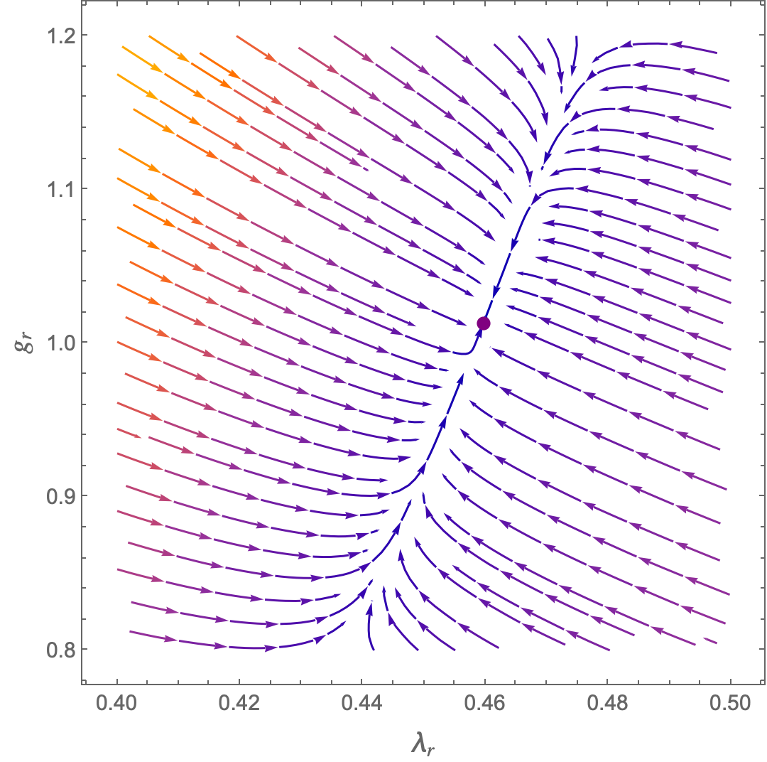
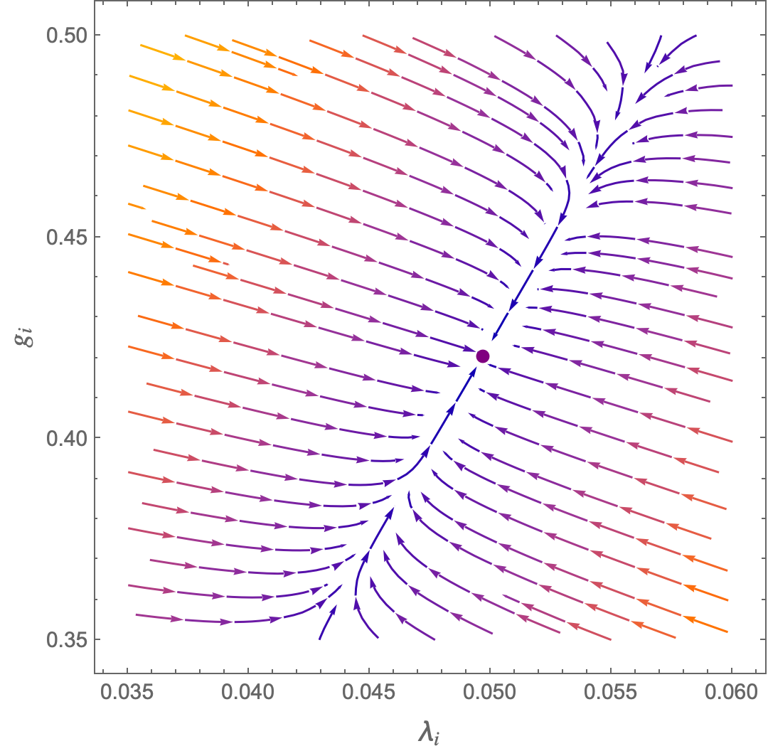
Figure 1: Projected flow diagram of the real (left) and imaginary (right) part in the $\lambda-g$ plane. The purple dot represents the fixed point in (3.34). The arrows point towards an increasing $k$, hence at $k\to\infty$ the fixed point is attractive in both projections.

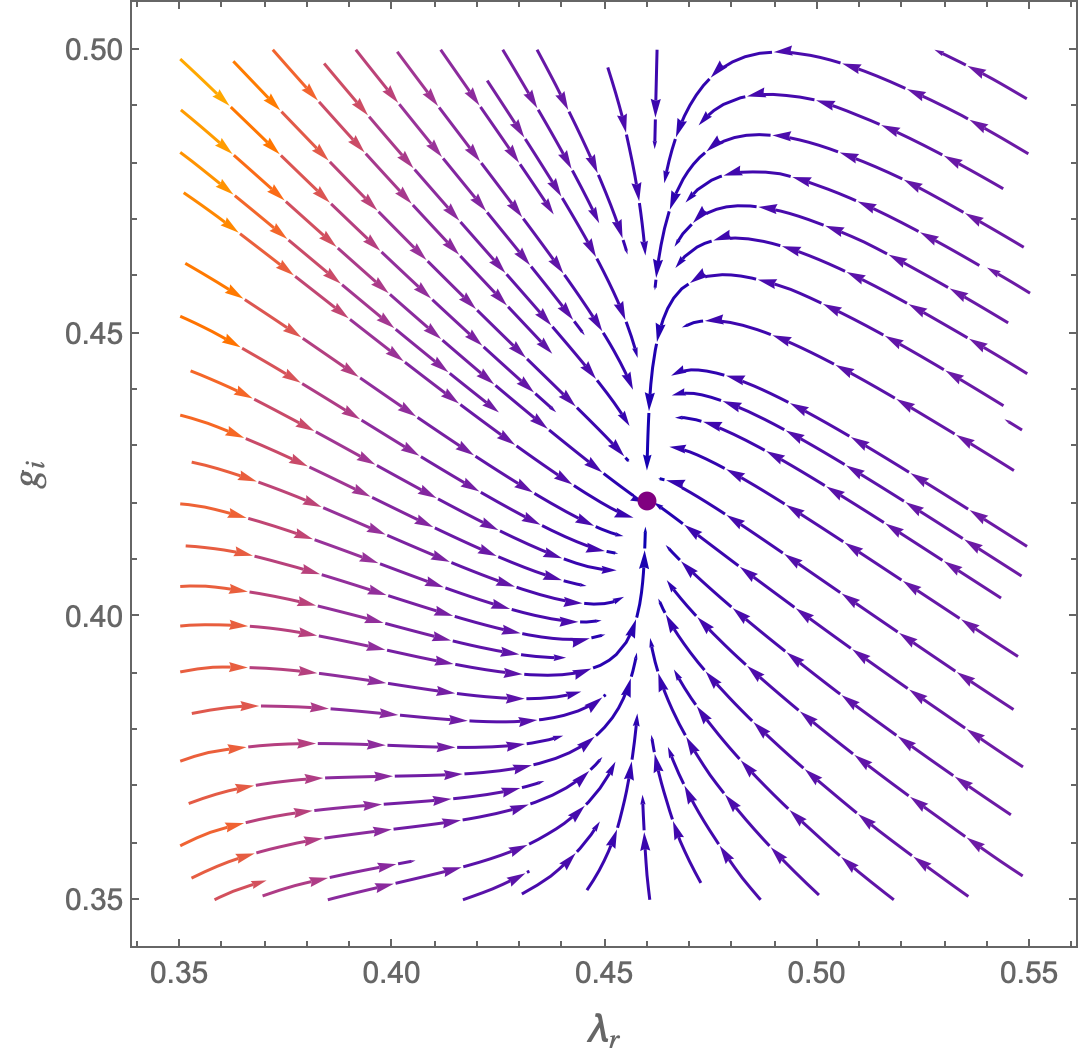
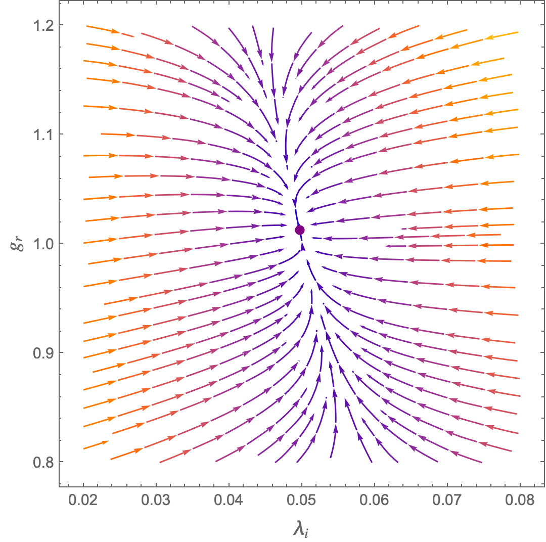
Figure 2: Flow diagram of the $\lambda_{\text{real}}-g_{\text{imaginary}}$ (left) and $\lambda_{\text{imaginary}}-g_{\text{real}}$ (right) part. The arrows along the trajectories point towards increasing value of $k$, and that means that the trajectories flow into the fixed point (3.34) in the UV.

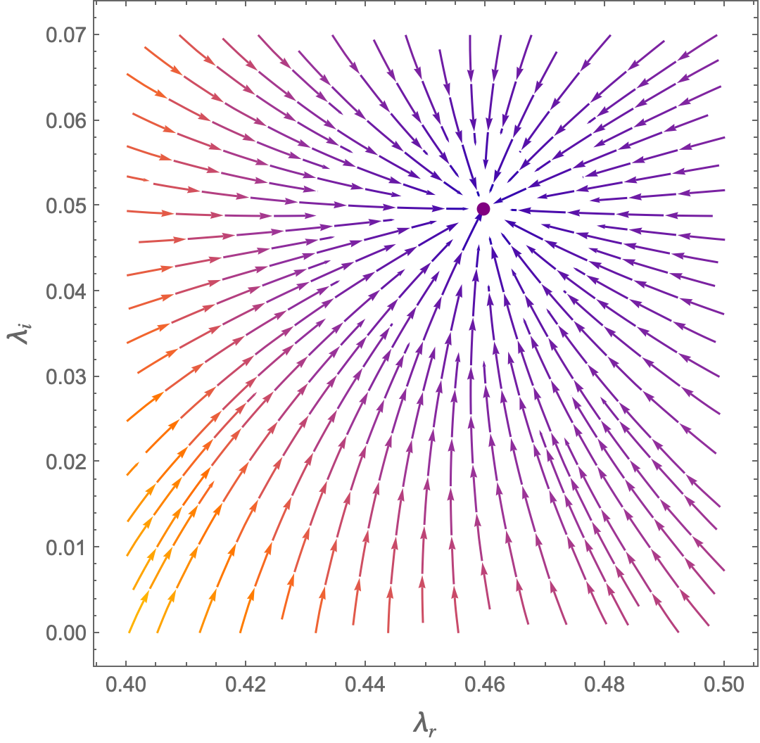
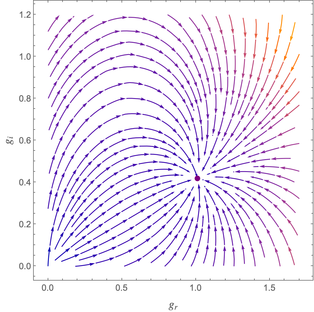
Figure 3: Flow diagram in the $\lambda_{\text{real}}-\lambda_{\text{imaginary}}$ (left, projected to $g=g_{\ast}$) and in the $g_{\text{real}}-g_{\text{imaginary}}$ (right, projected to $\lambda=\lambda_{\ast}$) space. The purple dot depicted is the fixed point in (3.34). The arrows point towards $k\to\infty$.

In all the 6 projections studied, the trajectories flow into the fixed point for $k\to\infty$.

Another interesting quantity carrying information about the nature of the fixed point are the critical exponents. The critical exponents can be computed by linearizing the flow around the fixed point, computing the stability matrix and determining its eigenvalues. The critical exponents for the Lorentzian UV fixed point (3.34) are

$$\theta_{1}=12.24-0.07\;i\;,\qquad\theta_{2}=0.95+0.017\;i\,,$$ (3.35)

therefore, being their real part positive, both coupling constants are associated to two relevant directions. Here the convenvention is that in the diagonalised form the couplings behave near the fixed point as $g_{j}(k)-g_{j}^{\ast}\propto(k_{0}/k)^{\theta_{j}}$ where $k_{0}$ is the point at which one sets initial conditions. That is, for $\Re(\theta_{j})>0$ the fixed point is reached insensitive to the initial condition, the coupling must not be fine tuned and thus must be measured (therefore it is relevant). Note that we do not expect here the critical exponents to be complex conjugated as in the standard FRG-ASQG treatment because of the intrinsically complex nature of the flow.

3.5 IR limit of the dimensionful couplings and admissible trajectories

Being interested in the full effective action, which corresponds to the $k\to 0$ limit, it is important to prove the existence of admissible trajectories, i.e., those trajectories for which $G_{k=0}=\text{real}$ and $\Lambda_{k=0}=\text{real}$. Fixing an arbitrary initial condition at a chosen scale $\bar{k}=1$ for $\lambda_{\text{real}}$ and $g_{\text{real}}$ (preferably closed to the UV fixed point) we can integrate down the flow and fine tune the initial data value of $\lambda_{\text{imaginary}}$ and $g_{\text{imaginary}}$ s.t. $\text{Im}[G_{k=0}]=0$ and $\text{Im}[\Lambda_{k=0}]=0$. This fine tuning is equivalent to computing the maps

$$\lambda_{\text{imaginary}}\big{|}_{k=\bar{k}} = f_{1}(\lambda_{\text{real}},g_{\text{real}})\big{|}_{k=\bar{k}}\;,$$ (3.36)

$$g_{\text{imaginary}}\big{|}_{k=\bar{k}} = f_{2}(\lambda_{\text{real}},g_{\text{real}})\big{|}_{k=\bar{k}}\;,$$ (3.37)

thereby reducing the flow by a dimension of 2. We have just started to investigate this very interesting question which has to be performed numerically. For instance it could be that there are domains in the real $(g,\lambda)$ plane such that there exists precisely one, several or no solution of the fine tuning problem in the imaginary $(g,\lambda)$ plane.

However, we can confirm numerically that admissible trajectories exist. We have analysed the existence of admissible trajectories by picking as real initial condition values of $g_{\text{real}}$ and $\lambda_{\text{real}}$ close to (the real part of) the UV fixed point value. In particular, as a first test, we establish the existence of admissible trajectories by exploring real initial conditions in the 5% neighbourhood of the fixed point value and by fine tuning the imaginary initial conditions at that chosen scale.

As an example, we select a trajectory with initial conditions $\lambda_{\text{real}}(k=1)\approx\lambda_{\ast}$ and $g_{\text{real}}(k=1)\approx g_{\ast}$ at $\bar{k}=1$. By fine tuning, we find the corresponding $\lambda_{\text{imaginary}}(k=1)=0.02$ and $g_{\text{imaginary}}(k=1)=0.11$, realizing an admissible trajectory (see Figures 4, 5). Furthermore, we tested that this trajectory flows into the UV fixed point. This can be appreciated in the plots of the dimensionless coupling in Figures 6 and 7.

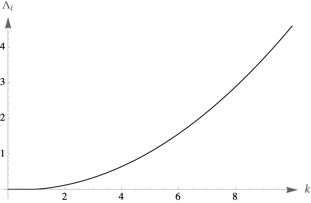
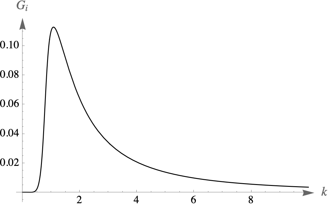
Figure 4: Admissible trajectory with $\lambda(k=1)=0.460+0.02i$ and $g(k=1)=1.013+0.11i$. The flow of the imaginary parts of the dimensionful coupling constants are vanishing for $k\to 0$.

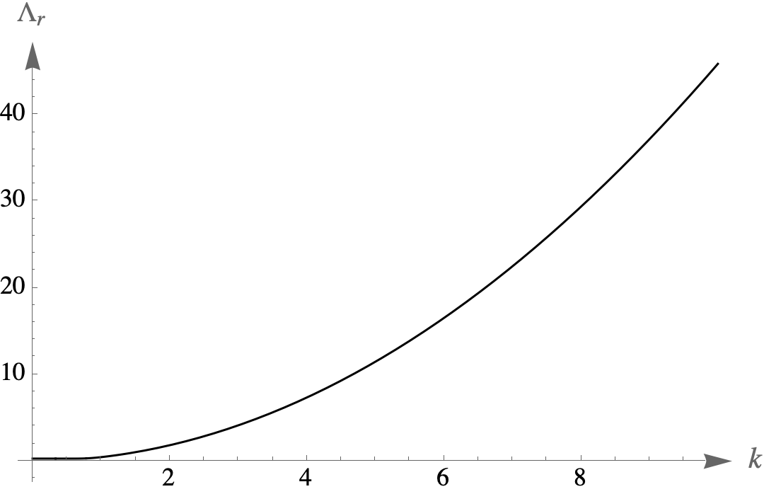
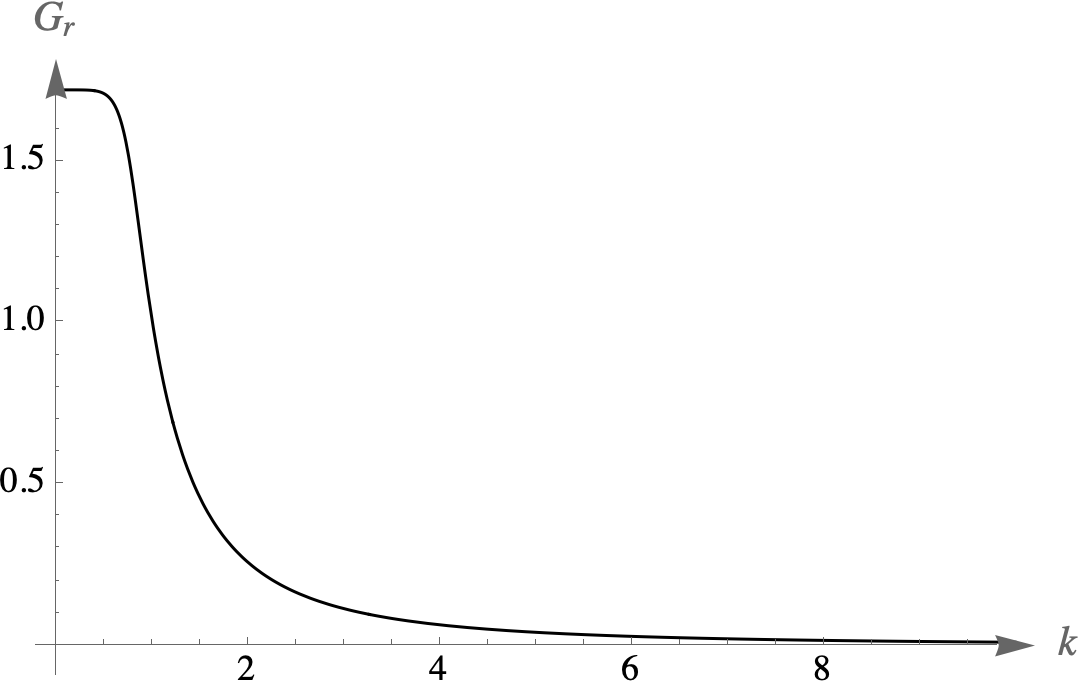
Figure 5: Admissible trajectory with $\lambda(k=1)=0.460+0.02i$ and $g(k=1)=1.013+0.11i$. The real part of the dimensionful coupling constants is well behaved and reaches a finite value (vanishes for $\Lambda_{\text{real}}$) when $k\to 0$.

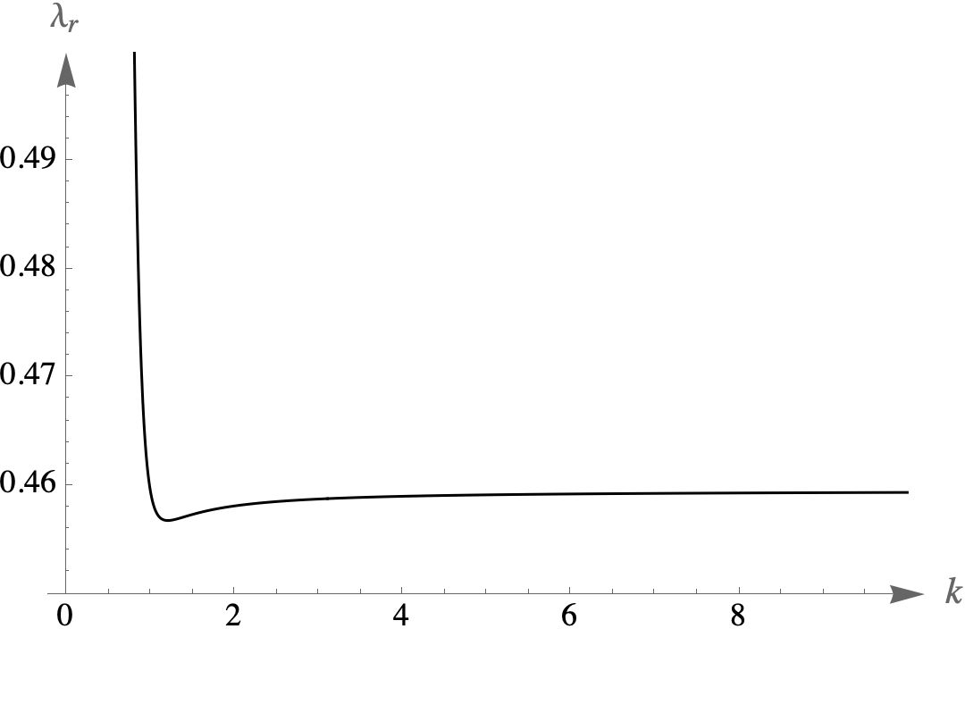
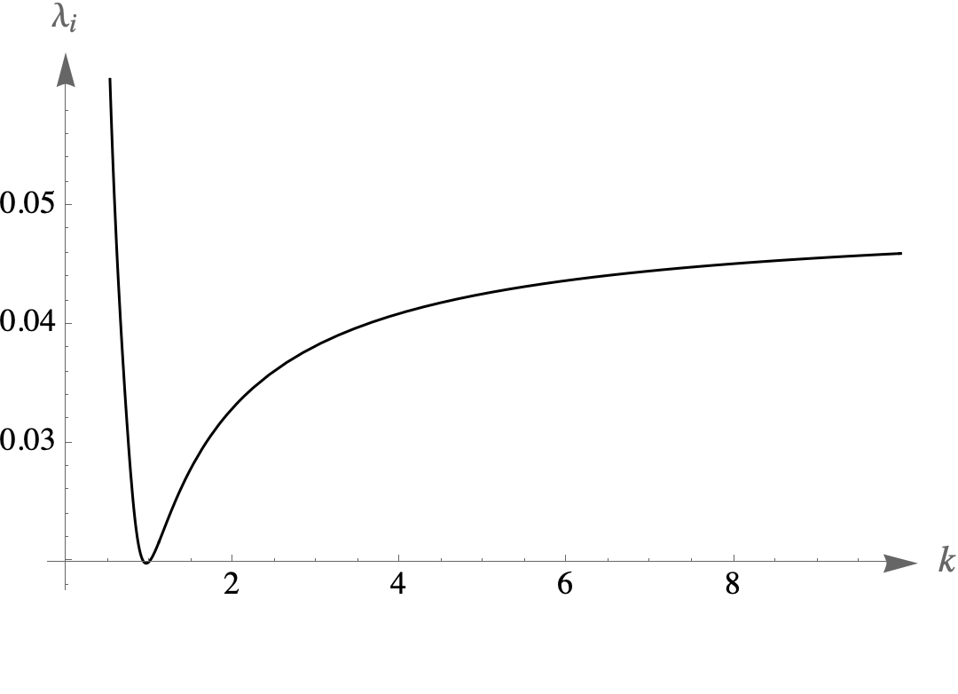
Figure 6: Admissible trajectory with $\lambda(k=1)=0.460+0.02i$ and $g(k=1)=1.013+0.11i$. The flow of the real and imaginary parts of the dimensionless coupling $\lambda_{k}$ is reaching the UV fixed point when $k\to\infty$. Note the divergence for vanishing $k$ due to the approximation (3.2) performed in the evaluation of the integrals.

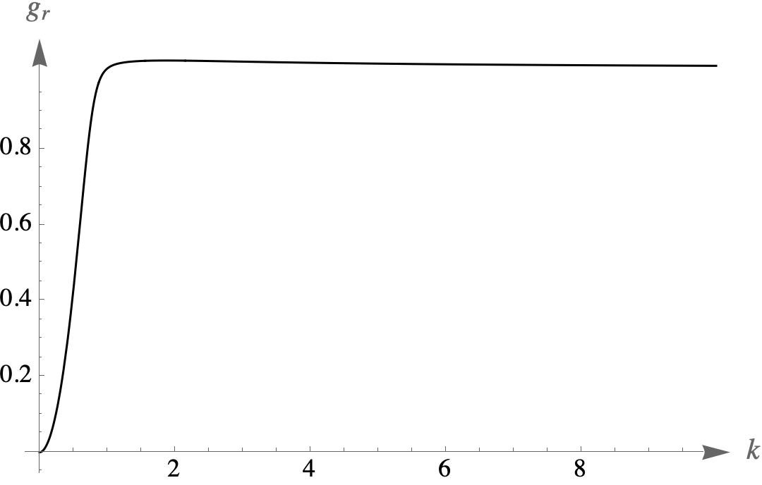
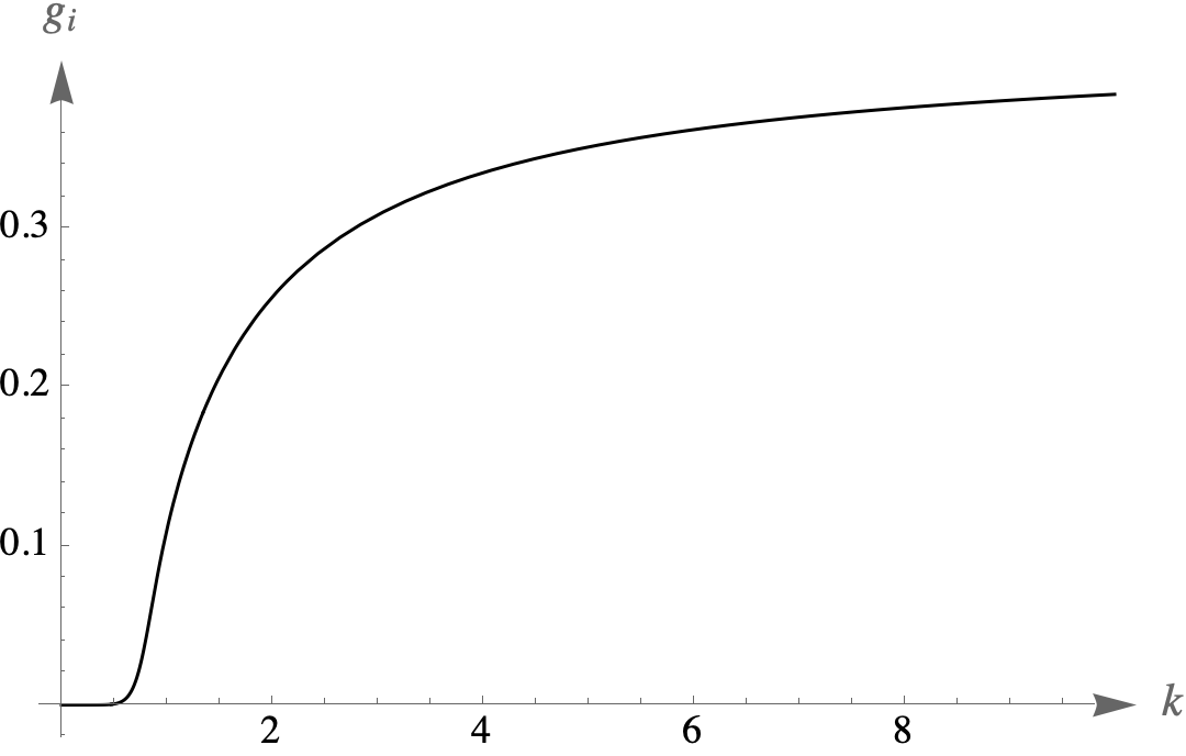
Figure 7: Admissible trajectory with $\lambda(k=1)=0.460+0.02i$ and $g(k=1)=1.013+0.11i$ and $g(k=1)=g_{\ast}+0.11i$. The real and imaginary parts of the dimensionless coupling $g_{k}$ flow into the UV fixed point when $k\to\infty$. In the IR both parts vanish.

4 Conclusion

In this contribution we considered a certain Einstein-Klein-Gordon theory as a showcase model to demonstrate that the ASQG and CQG approaches can be fruitfully combined. In particular, CQG gives important input for how to actually define the class of EEA to start with, displaying new contributions coming from 1. the state underlying the Hamiltonian quantum theory, 2. measure factors coming from the momentum integrals, 3. restrictions on correlation functions of the true degrees of freedom only and 4. that Lorentzian signature is the most natural choice.

ASQG on the other hand offers a systematic procedure for how to obtain a well defined effective action from which all the time ordered correlators of the Hamiltonian theory can be computed. The effective action can be argued to be a complete definition of the theory.

By exploiting the techniques for the Lorentzian heat kernel and introducing a new cut-off function, we computed the Lorentzian flow of an Einstein-Klein-Gordon model. Our analysis can be summarised in the following results:
1. We found that the coupling constant related to the matter contribution does not flow and also does not affect the flow of the gravitational coupling in the truncation considered here. 2. We computed the flow of Newton’s constant and the cosmological constant and we found an attractive UV fixed point at the value $\lambda_{*}=0.460+0.050\;i\;,g_{*}=1.013+0.420\;i$. Furthermore, we computed the critical exponents and related the coupling constant to two relevant directions.
3. We proved the existence of admissible trajectories, integrating down the flow to $k\to 0$ and finding trajectories which flow from real valued dimensional couplings in the IR and reach the UV fixed point of the dimensionless couplings when $k\to\infty$.

Among the many directions for future work are: Investigation of the space of admissible trajectories for the present model, classification of the Lorentzian cut-off functions with respect to their necessary physical and mathematical properties, incorporation of the flow of the ghost matrix term and its dependence on the state $\omega$, higher order truncations, more realistic matter coupling and the Euclidian version which is in principle possible but more complicated except for very special matter such as [23].

References

- [1]
-
[2]
R. Percacci. An introduction to covariant quantum gravity and asymptotic
safety. World Scientific, Singapore, 2017.
M. Reuter, F. Saueressig. Quantum gravity and the functional renormalization group. Cambridge monographs on mathematical physics, Cambridge, 2019.
A. Bonanno, A. Eichhorn, H. Gies, J. M. Pawlowski, R. Percacci, M. Reuter, F. Saueressig and G. P. Vacca, Critical reflections on asymptotically safe gravity, Front. in Phys. 8 (2020), 269 [arXiv:2004.06810 [gr-qc]]. -
[3]
C. Rovelli. Quantum Gravity. Cambridge University
Press, Cambridge, 2004.
T. Thiemann. Modern Canonical Quantum General Relativity. Cambridge University Press, Cambridge, 2007.
J. Pullin, R. Gambini. A first course in Loop Quantum Gravity. Oxford University Press, New York, 2011.
C. Rovelli, F. Vidotto. Covariant Loop Quantum Gravity. Cambridge University Press, Cambridge, 2015. - [4] T. Thiemann. Asymptotically safe – canonical quantum gravity junction.
-
[5]
E. Manrique, S. Rechenberger, F. Saueressig.
Asymptotically Safe Lorentzian Gravity.
Phys. Rev. Lett. 106 (2011) 251302. arXiv:1102.5012 [hep-th].
J. Biemans, A. Platania and F. Saueressig, Quantum gravity on foliated spacetimes: Asymptotically safe and sound, Phys. Rev. D 95 (2017) no.8, 086013 [arXiv:1609.04813 [hep-th]].
F. Saueressig and J. Wang, Foliated asymptotically safe gravity in the fluctuation approach,’JHEP 09 (2023), 064 [arXiv:2306.10408 [hep-th]].
G. Korver, F. Saueressig and J. Wang, Global Flows of Foliated Gravity-Matter Systems, [arXiv:2402.01260 [hep-th]]. -
[6]
E. D’Angelo, N. Drago, N. Pinamonti and K. Rejzner,
An Algebraic QFT Approach to the Wetterich Equation on Lorentzian Manifolds,
Annales Henri Poincare 25 (2024) no.4, 2295-2352
[arXiv:2202.07580 [math-ph]].
E. D’Angelo and K. Rejzner, A Lorentzian renormalisation group equation for gauge theories, [arXiv:2303.01479 [math-ph]].
E. D’Angelo. Asymptotic safety in Lorentzian quantum gravity. Phys. Rev. D 109 (2024) 06601211 [arXiv:2310.20603 [hep-th]]. - [7] R. Banerjee and M. Niedermaier, The spatial Functional Renormalization Group and Hadamard states on cosmological spacetimes, Nucl. Phys. B 980 (2022), 115814 [arXiv:2201.02575 [hep-th]].
- [8] J. Fehre, D. F. Litim, J. M. Pawlowski and M. Reichert, Lorentzian Quantum Gravity and the Graviton Spectral Function, Phys. Rev. Lett. 130 (2023) no.8, 081501 [arXiv:2111.13232 [hep-th]].
- [9] A. Baldazzi, R. Percacci and V. Skrinjar, Quantum fields without Wick rotation, Symmetry 11 (2019) no.3, 373 [arXiv:1901.01891 [gr-qc]].
- [10] L.F. Abbott. Introduction to the Background Field Method. Acta Phys. Polon. B 13 (1982) 33
- [11] T. Thiemann. Canonical quantum gravity, constructive QFT and renormalisation. Front. in Phys. 8 (2020) 548232, Front. in Phys. 0 (2020) 457 [arXiv:2003.13622 [gr-qc]]. v
- [12] J. E. Daum and M. Reuter, Einstein-Cartan gravity, Asymptotic Safety, and the running Immirzi parameter, Annals Phys. 334 (2013), 351-419 [arXiv:1301.5135 [hep-th]].
- [13] A. Baldazzi, K. Falls and R. Ferrero, Relational observables in asymptotically safe gravity, Annals Phys. 440 (2022), 168822 [arXiv:2112.02118 [hep-th]].
-
[14]
C. Wetterich, Exact evolution equation for the effective potential, Phys. Lett. B 301 (1993), 90-94 [arXiv:1710.05815 [hep-th]].
M. Reuter and C. Wetterich, Effective average action for gauge theories and exact evolution equations, Nucl. Phys. B 417 (1994), 181-214.
T. R. Morris, The Exact renormalization group and approximate solutions, Int. J. Mod. Phys. A 9 (1994), 2411-2450 [arXiv:hep-ph/9308265 [hep-ph]]. - [15] M. Reuter, Nonperturbative evolution equation for quantum gravity, Phys. Rev. D 57 (1998), 971-985 [arXiv:hep-th/9605030 [hep-th]].
-
[16]
L. E. Parker and D. Toms, Quantum Field Theory in Curved Spacetime: Quantized Field and Gravity, Cambridge University Press, 2009.
S. M. Christensen, Vacuum Expectation Value of the Stress Tensor in an Arbitrary Curved Background: The Covariant Point Separation Method, Phys. Rev. D 14 (1976), 2490-2501.
V. Moretti, Proof of the symmetry of the off diagonal heat kernel and Hadamard’s expansion coefficients in general C**(infinity) Riemannian manifolds, Commun. Math. Phys. 208 (1999), 283-309 [arXiv:gr-qc/9902034 [gr-qc]].
Y. Decanini and A. Folacci, Off-diagonal coefficients of the Dewitt-Schwinger and Hadamard representations of the Feynman propagator, Phys. Rev. D 73 (2006), 044027 [arXiv:gr-qc/0511115 [gr-qc]]. - [17] J. Glimm and A. Jaffe. Quantum Physics. Springer Verlag, New York, 1987.
- [18] K. Giesel, A. Vetter. Reduced loop quantization with four Klein–Gordon scalar fields as reference matter. Class. Quant. Grav. 36 (2019) 14, 145002 [arXiv:1610.07422 [gr-qc]].
-
[19]
D. Benedetti, K. Groh, P. F. Machado, F. Saueressig.
The Universal RG Machine. JHEP 1106 (2011) 079. arXiv:1012.3081 [hep-th].
K. Groh, F. Saueressig and O. Zanusso, Off-diagonal heat-kernel expansion and its application to fields with differential constraints, [arXiv:1112.4856 [math-ph]].
R. Ferrero, M. B. Fröb and W. C. C. Lima, Heat kernel coefficients for massive gravity, [arXiv:2312.10816 [hep-th]]. - [20] A. N. Bernal and M. Sanchez, On Smooth Cauchy hypersurfaces and Geroch’s splitting theorem, Commun. Math. Phys. 243 (2003), 461-470 [arXiv:gr-qc/0306108 [gr-qc]].
- [21] R. M. Wald, General Relativity, The University of Chicago Press, Chicago, 1989.
- [22] O. Bratteli, D. W. Robinson, Operator Algebras and Quantum Statistical Mechanics, vol. 1,2, Springer Verlag, Berlin, 1997
- [23] K. V. Kuchar, C. G. Torre, Gaussian reference fluid and interpretation of quantum geometrodynamics. Phys. Rev. D43 (1991) 419-441.
- [24] M. Henneaux, C. Teitelboim. Quantisation of Gauge Systems. Princeton University Press, Princeton, 1992.
-
[25]
P. Donà, A. Eichhorn and R. Percacci,
Matter matters in asymptotically safe quantum gravity,
Phys. Rev. D 89 (2014) no.8, 084035
[arXiv:1311.2898 [hep-th]].
K. Falls, D. F. Litim, K. Nikolakopoulos and C. Rahmede, Further evidence for asymptotic safety of quantum gravity, Phys. Rev. D 93 (2016) no.10, 104022 [arXiv:1410.4815 [hep-th]]. -
[26]
A. Bonanno and M. Reuter, Proper time flow equation for gravity,
JHEP 02 (2005), 035 [arXiv:hep-th/0410191 [hep-th]].
A. Bonanno, S. Lippoldt, R. Percacci and G. P. Vacca, On Exact Proper Time Wilsonian RG Flows, Eur. Phys. J. C 80 (2020) no.3, 249 [arXiv:1912.08135 [hep-th]].