Decentralized Synthesis of Passivity-Based Distributed Controllers for DC Microgrids

Abstract

Microgrids (MGs) provide a promising solution for exploiting renewable energy resources (RESs). Most of the existing papers on DC MGs focused on controller design. However, in this paper, we proposed a co-design passivity-based control (PBC) which design the controller and communication topology simultaneously. In addition, the plug-and-play feature is maintained without compromising the stability and re-designing of the remaining controllers. To this end, the local controller for distributed generators (DGs) and lines are obtained using smaller decentralized LMI problems and then the global controller is formulated using the passivity indices of the local controller to restore voltages to the reference value.

I Introduction

Microgrids, localized power systems with the ability to generate and manage their loads independently, are gaining recognition, especially in the realm of Direct Current (DC) microgrids, driven by challenges in frequency synchronization in AC MGs and the rising demand for DC loads. Hierarchical control structures have emerged as a standard approach for managing these microgrids, stratified into primary, secondary, and tertiary levels. At the primary level, known as the local controller, local data is utilized to regulate the DC bus voltage and ensure equitable power sharing among distributed generators (DGs). The secondary controller, operating with a slower response time, compensates for voltage deviations caused by the primary level. Its primary objective is to restore the voltage on the DC bus and ensure appropriate current sharing among DGs. The tertiary control level oversees power flow management and energy planning.

These control levels can be implemented in centralized, decentralized, or distributed manners. Centralized secondary control, governed by a central controller, offers precise, flexible, and reliable control performance. However, it is susceptible to single points of failure and lacks plug-and-play capability. In contrast, decentralized secondary control operates without direct communication. Although it eliminates the need for global information, it may face challenges in effectively coordinating DGs due to the lack of inter-device communication. On the other hand, distributed control relies on a sparse communication network to facilitate information exchange among neighboring DGs.

In [1], the authors considered the application of passivity theory to the voltage stabilization of DC microgrids including non-linear ZIP loads and dynamic RLC loads. They considered the PnP decentralized multivariable PI controllers and showed that they passivated the generation units and associated loads under certain conditions. The proposed control synthesis requires only the knowledge of DGs’ local parameters, which allows the PnP scenario. Compared with [2], they provide explicit inequalities for computing control gain instead of Linear Matrix Inequality (LMI). These inequalities only depend on the electrical parameters of the corresponding DG. In [2], a decentralized control method is designed where the primary control is developed in a PnP fashion in which the only global quantity used in the synthesis algorithm is a scalar parameter and the design of the local controller is line-independent. Therefore, there is no requirement to update the controllers of neighboring DGs.

In [3], the problem of designing distributed controllers to guarantee dissipativity of dynamically coupled subsystems. They provide distributed subsystem-level dissipativity analysis conditions and then use these conditions to synthesize controllers locally. They also make this synthesis composition to ensure the dissipativity of the system while adding new subsystems. This paper addressed three problems: 1) distributed analysis which decomposes a centralized dissipativity condition into dissipativity of individual subsystems. In comparison with other papers, this article proposes a distributed dissipative analysis condition that only uses the knowledge of the subsystem dynamics and information about the dissipativity of its neighbors. 2) It then formulates a procedure to synthesize local controllers to guarantee dissipativity. 3) They then formulated a control synthesis procedure that is compositional. Therefore, when a new subsystem is added, the design procedure uses only the knowledge of the dynamics of the newly added subsystem and the dissipativity of its neighboring to synthesize local control inputs such that the new network is dissipative.

In the conference paper [4], a new distributed passivity-based control strategy for DC MGs has been proposed using a consensus-based algorithm to achieve average voltage regulation while proper current sharing. In comparison with other methods where the Laplacian matrix determined the network, the design of the communication network is independent of the topology of the microgrid. The stability analysis is achieved by solving the LMI problem. The idea of interconnection and damping assignment passivity-based control (IDA-PBC) has been proposed in [5, 6, 7]. The authors in [5] proposed a novel damping (suppression of power and current oscillations) control for V/I droop-controlled DC MGs. The damping controller is designed using the IDA-PBC. This idea comes from the fact that the conventional passivity-based control (PBC) is very sensitive to load variations. The paper [6] also used the idea in [5] where a new decentralized control method based on passivity control is proposed for two DC distributed energy sources supplying the DC MG. The paper [7] also used the idea of IDA-PBC to improve the damping of the system. The application of this paper is battery where despite the variation of irradiation, the bus voltage and power remain constant by finding the irradiation levels through simulation for which the battery charges and discharges and remains idle.

A new passivity-based control approach for DC MGs is proposed in [8]. This approach is a data-driven control design and thus model-free and bypasses mathematical models to represent the network and guarantees stability. The authors in [9, 10, 11] proposed a robust PBC to solve the instability problem of constant power loads (CPLs) by adding the nonlinear disturbance observer (NDO). This paper aims to achieve 1) stabilize and regulate the DC-bus voltage using PBC 2) by combining the NDO with PBC, the steady-state error will be eliminated through the feedforward channel and improve the control robustness against CPL variations and 3) eliminate the voltage mismatch between the parallel connected converters using I-V droop control.

In the paper [12], an adaptive passivity-based controller (PBC) alongside an adaptive extended Kalman Filter (AEKF) is presented for DC MGs. The proposed controller estimates the unknown CPL power and prevents the number of measurement sensors. The main contribution of paper [13] is presenting a power-voltage droop controller in DC MG under explicit consideration of the electrical networked dynamics. Inspired by passivity-based control design, dissipation equality is derived in terms of the shifted Hamiltonian gradient. In the paper [14], a comprehensive passivity-based stability criterion is introduced by considering all input perturbations which provides a generic criterion for each individual interface converter.

I-A Main Contribution

In this paper, a passivity-based control (PCB) approach is developed in a decentralized manner. Additionally, a distributed control algorithm is utilized within the communication channels to accomplish two main objectives in DC MGs: voltage restoration and current sharing. main contributions of this paper can be outlined as follows:

I-B Organization

The structure of this paper is as follows: Section II provides an overview of several essential notations and foundational concepts related to the configurations of dissipativity and networked systems. Section III discusses the formulation of DC microgrid modeling, while Section IV delves into the modeling of networked systems. In Section V, the proposed passivity-based control is introduced. Finally, Section VI provides a conclusion.

II Preliminaries

II-A Notations

The notation $\mathbb{R}$ and $\mathbb{N}$ signify the sets of real and natural numbers, respectively. For every $N\in\mathbb{N}$, we define $\mathbb{N}_{N}\triangleq\{1,2,..,N\}$. A block matrix $A$ with dimensions $n\times m$ can be denoted as $A=[A_{ij}]_{i\in\mathbb{N}_{n},j\in\mathbb{N}_{m}}$, where $A_{ij}$ represents the $(i,j)^{\text{th}}$ block of $A$. It is worth noting that either subscripts or superscripts can be used for indexing, for example, $A_{ij}=A^{ij}$. $[A_{ij}]_{j\in\mathbb{N}_{m}}$ and $\text{diag}([A_{ii}])_{i\in\mathbb{N}_{n}}$ represent a block row matrix and a block diagonal matrix, respectively. $A^{\top}$ represents the transpose of a matrix $A$, and $(A^{\top})^{-1}=A^{-\top}$. $\mathbf{0}$ and $\mathbf{I}$ stand for the zero and identity matrices, respectively. The representation of a symmetric positive definite (semi-definite) matrix $A\in\mathbb{R}^{n\times n}$ is $A=A^{\top}>0\ (A=A^{\top}\geq 0)$.

II-B Dissipativity

Consider a dynamic control system

$$\dot{x}(t)=f(x(t),u(t)),$$ (1)

$$y(t)=h(x(t),u(t)),$$

where $x(t)\in\mathbb{R}^{n}$, $u(t)\in\mathbb{R}^{q}$, $y(t)\in\mathbb{R}^{m}$, and $f:\mathbb{R}^{n}\times\mathbb{R}^{q}\rightarrow\mathbb{R}^{n}$ and $h:\mathbb{R}^{n}\times\mathbb{R}^{q}\rightarrow\mathbb{R}^{m}$ are continuously differentiable. Eq. (1) has an equilibrium point when there is a unique $u^{*}\in\mathbb{R}^{q}$ such that $f(x^{*},u^{*})=0$ for all $x^{*}\in\mathcal{X}$, where $\mathcal{X}\subset\mathbb{R}^{n}$. Both $u^{*}$ and $y^{*}\triangleq h(x^{*},u^{*})$ are implicit functions of $x^{*}$. These conditions are met for every $x^{*}\in\mathcal{X}$. The equilibrium-independent-dissipativity (EID) feature [15], which is described below, may be employed for the dissipativity analysis of (1) without the explicit knowledge of its equilibrium points.
Definition 1. If there is a continuously differentiable storage function $V:\mathbb{R}^{n}\times\mathcal{X}\rightarrow\mathbb{R}$, the system is known as EID under supply rate $s:\mathbb{R}^{q}\times\mathbb{R}^{m}\rightarrow\mathbb{R}$. For all $(x,x^{*},u)\in\mathbb{R}^{n}\times\mathcal{X}\times\mathbb{R}^{q}$, $V(x,x^{*})>0$ with $x\neq x^{*}$, $V(x^{*},x^{*})=0$, and $\dot{V}(x,x^{*})=\nabla_{x}V(x,x^{*})f(x,u)\leq s(u-u^{*},y-y^{*})$.

Depending on the utilized supply rate $s(.,.)$, this EID property may be specialized. The concept of the $X-\text{EID}$ property is used in the sequel. This property is characterized by a quadratic supply rate, which is determined by the coefficient matrix $X=X^{\top}\in\mathbb{R}^{q+m}$.
Definition 2. If the system (1) is EID under the quadratic supply rate, it is called $X-\text{EID}$ with $X\triangleq[X^{kl}]_{k,l\in\mathbb{N}_{2}}$:

$$s(u-u^{*},y-y^{*})\triangleq\begin{bmatrix}u-u^{*}\\ y-y^{*}\end{bmatrix}^{\top}\begin{bmatrix}X^{11}&X^{12}\\ X^{21}&X^{22}\end{bmatrix}\begin{bmatrix}u-u^{*}\\ y-y^{*}\end{bmatrix}$$

Remark 1.

If the system (1) is $X-\text{EID}$ with:
1) $\begin{bmatrix}\mathbf{0}&\frac{1}{2}\mathbf{I}\\ \frac{1}{2}\mathbf{I}&\mathbf{0}\end{bmatrix}$, then it is passive;
2) $\begin{bmatrix}-\nu\mathbf{I}&\frac{1}{2}\mathbf{I}\\ \frac{1}{2}\mathbf{I}&-\rho\mathbf{I}\end{bmatrix}$, then it is strictly passive ($\nu$ and $\rho$ are the input feedforward and output feedback passivity indices, respectively);
3)  $\begin{bmatrix}\gamma^{2}\mathbf{I}&\mathbf{0}\\ \mathbf{0}&-\mathbf{I}\end{bmatrix}$, then it is $L_{2}$-stable ($\gamma$ is the $L_{2}$-gain, denoted as $L2G(\gamma)$).

If the system (1) is linear time-invariant (LTI), a necessary and sufficient condition for the system (1) to be X-EID is provided in the following proposition, which regards it as a linear matrix inequality (LMI) problem.

Proposition 1.

[16] The linear time-invariant (LTI) system

$$\dot{x}(t)= Ax(t)+Bu(t)$$ (2)

$$y(t)= Cx(t)+Du(t)$$

is $X$-EID if and only if there exists $P>0$ such that

$$\begin{bmatrix}-\mathcal{H}(PA)+C^{\top}X^{22}C&-PB+C^{\top}X^{21}+C^{\top}X^{22}D\\ \star&X^{11}+\mathcal{H}(X^{12}D)+D^{\top}X^{22}D\end{bmatrix}\geq 0$$ (3)

The following corollary takes into account a specific LTI system that has a local controller (a setup that we will see later on) and gives an LMI problem for synthesizing this local controller to optimize or enforce X-EID.

Corollary 1.

[16] The LTI system

$$\dot{x}(t)=(A+BL)x(t)+\eta(t),$$ (4)

is $X-\text{EID}$ with $X^{22}<0$ from external input $\eta(t)$ to state $x(t)$ if and only if there exists $P>0$ and $K$ such that

$$\begin{bmatrix}-(X^{22})^{-1}&P&0\\ \star&-\mathcal{H}(AP+BK)&-I+PX^{21}\\ \star&\star&X^{11}\end{bmatrix}\geq 0$$ (5)

and $L=KP^{-1}$.

II-C Networked Systems

II-C1 Configuration

The networked system $\Sigma$ depicted in Fig. 1 is composed of $N$ independent dynamic subsystems $\{\Sigma_{i}:i\in\mathbb{N}_{N}\}$ and a static interconnection matrix $M$ that characterizes the interconnections between the subsystems, an exogenous input signal $w(t)\in\mathbb{R}^{r}$ (e.g. disturbance) and an interested output signal $z(t)\in\mathbb{R}^{l}$ (e.g. performance).

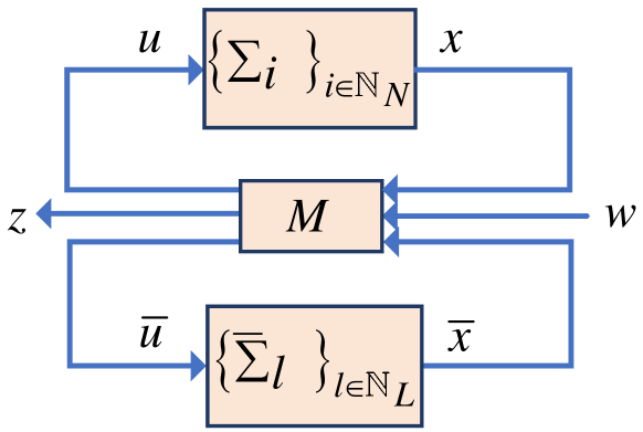
Figure 1: A generic networked system $\Sigma$

The dynamics of the subsystem $\{\Sigma_{i}:i\in\mathbb{N}_{N}\}$ are provided by

$$\dot{x}_{i}(t) =f_{i}(x_{i}(t),u_{i}(t)),$$ (6)

$$y_{i}(t) =h_{i}(x_{i}(t),u_{i}(t)),$$

where $x_{i}(t)\in\mathbb{R}^{n_{i}}$, $u_{i}(t)\in\mathbb{R}^{q_{i}}$, $y_{i}(t)\in\mathbb{R}^{m_{i}}$.
On the other hand, the interconnection matrix $M$ and the corresponding interconnection relationship are given by:

$$\begin{bmatrix}u\\ \bar{u}\\ z\end{bmatrix}=M\begin{bmatrix}y\\ \bar{y}\\ w\end{bmatrix}\equiv\begin{bmatrix}M_{uy}&M_{u\bar{y}}&M_{uw}\\ M_{\bar{u}y}&M_{\bar{u}\bar{y}}&M_{\bar{u}w}\\ M_{zy}&M_{z\bar{y}}&M_{zw}\end{bmatrix}\begin{bmatrix}y\\ \bar{y}\\ w\end{bmatrix}$$ (7)

where $u\triangleq[u_{i}^{\top}]^{\top}_{i\in\mathbb{N}_{N}}$ and $y\triangleq[y_{i}^{\top}]^{\top}_{i\in\mathbb{N}_{N}}$.

II-C2 Dissipativity Analysis

Inspired by [15], the following proposition exploits the $X_{i}$-EID properties of the individual subsystems $\Sigma_{i},i\in\mathbb{N}_{N}$ to formulate an LMI problem so as to analyze the Y-EID property of the networked system $\Sigma$, where $\text{Y}=\text{Y}^{\top}=[\text{Y}^{kl}],k,l\in\mathbb{N}_{2}$.

Remark 2.

A subsystem is required to be finite-gain $\mathcal{L}_{2}$ stable with some $\mathcal{L}_{2}$-gain $\gamma$ from its disturbance $w(t)$ to performance $z(t)$. This specification is equivalent to $\mathbf{Y}$-dissipativity with:

$$\mathbf{Y}=\begin{bmatrix}\gamma^{2}\mathbf{I}&0\\ 0&-\mathbf{I}\end{bmatrix}=\begin{bmatrix}\tilde{\gamma}\mathbf{I}&0\\ 0&-\mathbf{I}\end{bmatrix}$$ (8)

Let $\tilde{\gamma}\triangleq\gamma^{2}$, and we need $0<\tilde{\gamma}<\bar{\gamma}$, where $\bar{\gamma}\in\mathbb{R}>0$ is a constant value.

Proposition 2.

[16] Let $\hat{x}^{*}\triangleq[[x_{i}^{*}{{}^{\top}}]_{i\in\mathbb{N}_{N}},[\bar{x}_{i}^{*\top}]_{i\in\mathbb{N}_{\bar{N}}}]^{\top}$ be an equilibrium point of networked (under $w(t)=0$) with $x_{i}^{*}\in\mathcal{X}_{i},\forall i\in\mathbb{N}_{N}$, $\bar{x}_{i}^{*}\in\bar{\mathcal{X}}_{i},\forall i\in\mathbb{N}_{\bar{N}}$ and $z^{*}$ be corresponding output. Then, the network is Y-dissipative if there exist scalars $p_{i}\geq 0,\forall i\in\mathbb{N}_{N}$ and $\bar{p}_{i},i\in\mathbb{N}_{\bar{N}}$ such that

$$\begin{bmatrix}M_{uy}&M_{u\bar{y}}&M_{uw}\\ \mathbf{I}&\mathbf{0}&\mathbf{0}\\ M_{\bar{u}y}&M_{\bar{u}\bar{y}}&M_{\bar{u}w}\\ \mathbf{0}&\mathbf{I}&\mathbf{0}\\ \mathbf{0}&\mathbf{0}&\mathbf{I}\\ M_{zy}&M_{z\bar{y}}&M_{zw}\end{bmatrix}^{\top}\begin{bmatrix}X_{p}&\mathbf{0}&\mathbf{0}\\ \mathbf{0}&\bar{X}_{\bar{p}}&\mathbf{0}\\ \mathbf{0}&\mathbf{0}&-\mathbb{Y}\end{bmatrix}\star\leq 0,$$ (9)

where the components $X_{p}$ and $X_{\bar{p}}$ for $i\in\mathbb{N_{N}}$ are defined as follows:

$$X_{p}\triangleq\begin{bmatrix}\text{diag}(p_{i}X_{i}^{11})&\text{diag}(p_{i}X_{i}^{12})\\ \text{diag}(p_{i}X_{i}^{21})&\text{diag}(p_{i}X_{i}^{22})\end{bmatrix}$$ (10)

$$\bar{X}_{\bar{p}}\triangleq\begin{bmatrix}\text{diag}(\bar{p}_{i}\bar{X}_{i}^{11})&\text{diag}(\bar{p}_{i}\bar{X}_{i}^{12})\\ \text{diag}(\bar{p}_{i}\bar{X}_{i}^{21})&\text{diag}(\bar{p}_{i}\bar{X}_{i}^{22})\end{bmatrix}$$

II-C3 Topology Synthesis

The following proposition develops an LMI problem to synthesize the interconnection matrix $M$ (7) to enforce the $\mathbb{Y}$-EID property for the networked system $\Sigma$. Nonetheless, similar to [17], we must initially establish two mild assumptions.

Assumption 1.

For the networked system $\Sigma$, the provided Y-EID specification is such that $\textbf{Y}^{22}<0$.

Remark 3.

According to Rm. 1, As. 1 holds if the networked system $\Sigma$ must be either: (1) L2G($\gamma$) or (2) OFP($\rho$) (or IF-OFP($\nu,\rho$)) with some $\rho>0$, i.e., $L_{2}$-stable or passive, respectively. Therefore, As. 1 is mild since it is usually preferable to make the networked system $\Sigma$ either $L_{2}$-stable or passive.

Assumption 2.

Every subsystem $\Sigma_{i}$ in the networked system $\Sigma$ is $X_{i}$-EID with $X_{i}^{11}>0$ or $X_{i}^{11}<0,\forall i\in\mathbb{N}_{N}$.

Remark 4.

Based on Rm. 1, As. 2 holds if the networked subsystem $\Sigma_{i},i\in\mathbb{N}_{N}$ must be either: (1) L2G($\gamma_{i}$) (as $X_{i}^{11}=\gamma_{i}^{2}\mathbf{I}>0$), or (2) IFP($\nu_{i}$) (or IF-OFP($\nu_{i},\rho_{i}$)) with $\nu_{i}<0$ (i.e., non-passive), or (3) IFP($\nu_{i}$) (or IF-OFP($\nu_{i},\rho_{i}$)) with $\nu_{i}>0$ (i.e., passive). Thus, As. 2 is also mild.

Proposition 3.

Under Assumptions 1 and 2, the network system NSC 4 can be Y-EID ($\mathbf{Y}$-dissipative from $w(t)$ to output $z(t)$) by synthesizing the interconnection matrix $M$ by solving LMI problem:

Find: $$L_{uy},L_{u\bar{y}},L_{uw},L_{\bar{u}y},L_{\bar{u}\bar{y}},L_{\bar{u}w},M_{zy},M_{z\bar{y}},M_{zw},$$ (11)

$$\{p_{i}:i\in\mathbb{N}_{N}\},\{\bar{p}_{i}:i\in\mathbb{N}_{\bar{N}}\}$$

Sub. to: $$p_{i}\geq 0,\forall i\in\mathbb{N}_{N},\ \ \bar{p}_{i}\geq 0,\forall i\in\mathbb{N}_{\bar{N}},\ \text{and}\ \eqref{NSC4YEID},$$

with $\scriptsize\begin{bmatrix}M_{uy}&M_{u\bar{y}}&M_{uw}\\ M_{\bar{u}y}&M_{\bar{u}\bar{y}}&M_{\bar{u}w}\end{bmatrix}=\begin{bmatrix}\textbf{X}_{p}^{11}&\mathbf{0}\\ \mathbf{0}&\bar{\textbf{X}}_{\bar{p}}^{11}\end{bmatrix}^{-1}\begin{bmatrix}L_{uy}&L_{u\bar{y}}&L_{uw}\\ L_{\bar{u}y}&L_{\bar{u}\bar{y}}&L_{\bar{u}w}\end{bmatrix}$.

$$\begin{bmatrix}\textbf{X}_{p}^{11}&\mathbf{0}&\mathbf{0}&L_{uy}&L_{u\bar{y}}&L_{uw}\\ \mathbf{0}&\bar{\textbf{X}}_{\bar{p}}^{11}&\mathbf{0}&L_{\bar{u}y}&L_{\bar{u}\bar{y}}&L_{\bar{u}w}\\ \mathbf{0}&\mathbf{0}&-\textbf{Y}^{22}&-\textbf{Y}^{22}M_{zy}&-\textbf{Y}^{22}M_{z\bar{y}}&\textbf{Y}^{22}M_{zw}\\ L_{uy}^{\top}&L_{\bar{u}y}^{\top}&-M_{zy}^{\top}\textbf{Y}^{22}&-L_{uy}^{\top}\textbf{X}^{12}-\textbf{X}^{21}L_{uy}-\textbf{X}_{p}^{22}&-\textbf{X}^{21}L_{u\bar{y}}-L_{\bar{u}y}^{\top}\bar{\textbf{X}}^{12}&-\textbf{X}^{21}L_{uw}+M_{zy}^{\top}\textbf{Y}^{21}\\ L_{u\bar{y}}^{\top}&L_{\bar{u}\bar{y}}^{\top}&-M_{z\bar{y}}^{\top}\textbf{Y}^{22}&-L_{u\bar{y}}^{\top}\textbf{X}^{12}-\bar{\textbf{X}}^{21}L_{\bar{u}y}&-(L_{\bar{u}\bar{y}}^{\top}\bar{\textbf{X}}^{12}+\bar{\textbf{X}}^{21}L_{\bar{u}\bar{y}}+\bar{\textbf{X}}_{\bar{p}}^{22})&-\bar{\textbf{X}}^{21}L_{\bar{u}w}+M_{z\bar{y}}^{\top}\textbf{Y}^{21}\\ L_{uw}^{\top}&L_{\bar{u}w}^{\top}&-M_{zw}^{\top}\textbf{Y}^{22}&-L_{uw}^{\top}\textbf{X}^{12}+\textbf{Y}^{12}M_{zy}&-L_{\bar{u}w}^{\top}\bar{\textbf{X}}^{12}+\textbf{Y}^{12}M_{z\bar{y}}&M_{zw}^{\top}\textbf{Y}^{21}+\textbf{Y}^{12}M_{zw}+\textbf{Y}^{11}\end{bmatrix}>0$$ (12)

III DC Microgrid Modeling

The initial step involves explaining the electrical configuration of a DC MG, which consists of multiple DGs interconnected via power transmission lines. Specifically, we utilize the model proposed in the study by [1], which enables considering various topologies of DC MGs. The whole microgrid can be represented by a directed connected graph $\mathcal{G}=(\mathcal{V},\mathcal{E})$ where the $\mathcal{V}=\{1,...,N\}$ represents the set of nodes and $\mathcal{E}\subseteq(\mathcal{V}\times\mathcal{V})$ represents the set of edges. For a given node $i\in\mathcal{V}$, the set of out-neighbors is $\mathcal{N}_{i}^{+}=\{j\in\mathcal{V}:(i,j)\in\mathcal{E}\}$, the set of in-neighbors is $\mathcal{N}_{i}^{-}=\{j\in\mathcal{V}:(j,i)\in\mathcal{E}\}$, and the set of neighbors is $\mathcal{N}_{i}=\mathcal{N}_{i}^{+}\cup\mathcal{N}_{i}^{-}$. $\mathcal{V}$ is divided into two parts: $\mathcal{D}=\{1,..,n\}$ represents the set of DGs and $\mathcal{L}=\{n+1,...,n+m\}$ represents the set of transmission lines. The DGs are connected through the communication and physical interconnection power lines. If the DG $i$ is connected to DG $j$, then $(i,j)\in\mathcal{E}$. The $\Sigma_{i}^{DG},i\in\mathbb{N}_{N}$ represents an MG with $N$ DGs, and the $\Sigma_{l}^{line},l\in\mathbb{N}_{L}$ an MG with $L$ transmission lines. The interface between each DG and the power grid is established through a point of common coupling (PCC). The loads are assumed to be connected to the DG terminals for simplicity. Indeed, the loads can be moved to PCC using Kron reduction, even if they are in a different location [18]. Given that every DG is only directly connected to the lines, every edge in $\mathcal{E}$ has one node in $\mathcal{D}$ and another node in $\mathcal{L}$. This results in $\mathcal{G}$ being a bipartite graph. The orientation of each edge reflects an arbitrarily chosen reference direction for positive currents. A line must have both in-neighbors and out-neighbors since the current entering a line must exit it. Indeed, each node in $\mathcal{L}$ is connected via two directed edges to two distinct nodes in $\mathcal{D}$. The incidence matrix for a subsequent matrix is denoted by $B\in\mathbb{R}^{n\times m}$, where DGs are arranged in rows and lines are arranged in columns.

$$B_{il}=\begin{cases}+1&l\in\mathcal{N}_{i}^{+},\\ -1&l\in\mathcal{N}_{i}^{-},\ i\in\mathcal{D},l\in\mathcal{N},\\ 0&\text{otherwise}.\end{cases}$$ (13)

III-A Dynamic model of a DG

Each DG consists of a DC voltage source, a buck converter, and a series RLC filter. The $i$-th DG unit supplies power to a specific local load located at the $\text{PCC}_{i}$. Additionally, it is interconnected with other DG units via power transmission lines. Fig. 2 illustrates a schematic electric diagram of the $i$th DG system, including load, connecting lines, loads, and a local controller. By applying Kirchhoff’s Current Law (KCL) and Kirchhoff’s Voltage Law (KVL) on the DG side at the $\text{PCC}_{i}$, the following equations are derived for $\sum_{i}^{DG}$:

$$C_{ti}\frac{dV_{i}}{dt} =I_{ti}-I_{Li}(V_{i})-I_{i}$$ (14)

$$L_{ti}\frac{dI_{ti}}{dt} =-V_{i}-R_{ti}I_{ti}+V_{ti}$$

In (14), the symbol $V_{ti}$ represents the input command signal applied to the buck converter, while $I_{ti}$ denotes the current flowing through the filter. The variables $R_{ti}\in\mathbb{R}^{+}$, $L_{ti}\in\mathbb{R}^{+}$, and $C_{ti}\in\mathbb{R}^{+}$ represent the internal resistance, inductance, and capacitance of the DG converter, respectively.

III-B Dynamic model of power line

Each transmission line is modeled using the $\pi$-equivalent representation. The assumption is made that the line capacitances are consolidated with the capacitance of the DG filter. Hence, as seen in Fig. 2, the power line denoted as $l$ is represented by a RL circuit with a positive resistance $R_{l}$ and inductance $L_{l}$. By applying Kirchoff’s voltage law (KVL) to analyze the $l$-th power line denoted $\Sigma_{l}^{line}$, one can get:

$$\Sigma_{l}^{line}:\frac{dI_{l}}{dt}=-\frac{R_{l}}{L_{l}}I_{l}+\frac{1}{L_{l}}u_{l}$$ (15)

where $u_{l}=V_{i}-V_{j}=\sum_{i\in\mathcal{N}_{l}}B_{il}V_{i}$. The variables $V_{i}$ and $I_{l}$ denote the voltage at the $\text{PCC}_{i}$ and the current conducting through the $l$-th power line, respectively.

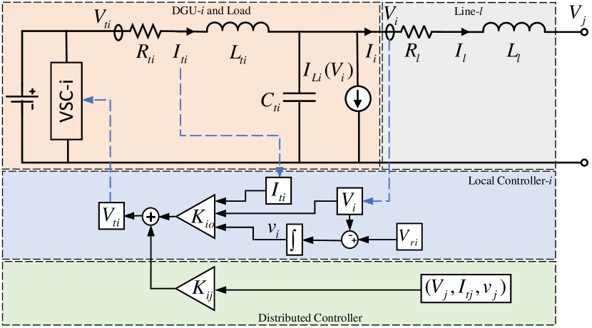
Figure 2: Electrical Schematic of DG-i, load-$i$, local controller-$i$, $i\in\mathcal{N}_{N}$ and line-$l$, $l\in\mathcal{N}_{L}$

The line current $I_{i}$ is the current injected into the DC MG and is given by:

$$I_{i}=\sum_{l\in\mathcal{N}_{i}^{+}}B_{il}I_{l}+\sum_{l\in\mathcal{N}_{i}^{-}}B_{il}I_{l}=\sum_{l\in\mathcal{N}_{i}}B_{il}I_{l}.$$ (16)

III-C Load model

The phrase $I_{Li}(V_{i})$ in Fig. 2 stands for the current flowing through the $i$-th load. The functional dependence on the PCC voltage varies depending on the type of load, and the term $I_{Li}(V_{i})$ has distinct expressions. The following load models are included: (1) loads with constant current: $I_{Lli}=\bar{I}_{Lli}$, (2) constant impedance loads $I_{LZi}(V_{i})=Y_{Li}V_{i}$, where the conductance of the $i$th load is $Y_{Li}=1/R_{Li}>0$, and (3) constant power loads $I_{LPi}(V_{i})=V_{i}^{-1}P_{Li}^{*}$, where $P_{Li}^{*}>0$ represents the power demand of the load $i$. Therefore, the ZIP loads are as follows:

$$I_{Li}(V_{i})=\bar{I}_{Li}+Y_{Li}V_{i}+V_{i}^{-1}P_{Li}^{*}$$ (17)

III-D State space model of DC MG

By integrating the DG dynamics in Eq. (14) and the error dynamic in Eq. (25), the state space representation of the DG will be obtained:

$$\sum_{i}^{DG}:\begin{cases}\dot{x}_{i}(t)=A_{i}x_{i}(t)+B_{i}u_{i}(t)+C_{i}d_{i}(t)+\xi_{i}(t)\\ z_{i}(t)=H_{i}x_{i}(t)\end{cases}$$ (18)

where $x_{i}=\begin{bmatrix}V_{i}&I_{ti}&v_{i}\end{bmatrix}^{\top}$ is the state, $u_{i}=V_{ti}$ is the control input, $d_{i}=\begin{bmatrix}\bar{I}_{Li}&0&V_{ri}\end{bmatrix}^{\top}$ stands for the exogenous input or disturbance, and $z_{i}=v_{i}$ is the desired performance since our goal is $\lim_{t\to\infty}V_{i}(t)=V_{ri}$ The term $\xi_{i}$ is the transmission line coupling corresponding to DG $i$. Thus, we have:

$$\frac{dV_{i}}{dt} =\frac{1}{C_{ti}}I_{ti}-\frac{1}{C_{ti}}I_{Li}(V_{i})-\frac{1}{C_{ti}}I_{i}$$

$$\frac{dI_{ti}}{dt} =-\frac{1}{L_{ti}}V_{i}-\frac{R_{ti}}{L_{ti}}I_{ti}+\frac{1}{L_{ti}}u_{i}$$ (19)

$$\frac{dv_{i}}{dt} =V_{i}-V_{ri}$$

III-E The local and global controller

The primary aim of the local controller is to guarantee that the voltage at ($\text{PCC}_{i}$) closely follows a predetermined reference voltage ($V_{ri}$), often supplied by a higher level controller. In the absence of voltage stabilization in the DC MG, there is a potential for voltages to exceed critical thresholds, leading to detrimental consequences for the loads and the DC MG infrastructure.

The state space representation of DC MG is obtained as follows by using Eq. (III-D):

$$\begin{bmatrix}\frac{dV_{i}}{dt}\\ \frac{dI_{ti}}{dt}\\ \frac{dv_{i}}{dt}\end{bmatrix}= \begin{bmatrix}-\frac{Y_{Li}}{C_{ti}}V_{i}-\frac{P_{Li}}{C_{ti}}V_{i}^{-1}+\frac{1}{C_{ti}}I_{ti}\\ -\frac{1}{L_{ti}}V_{i}-\frac{R_{ti}}{L_{ti}}I_{ti}+\frac{1}{L_{ti}}f_{io}\\ V_{i}\end{bmatrix}+\begin{bmatrix}-\frac{\bar{I}_{Li}}{C_{ti}}\\ 0\\ -V_{ri}\end{bmatrix}$$ (20)

$$+ \begin{bmatrix}-\frac{1}{C_{ti}}\sum B_{il}I_{l}\\ 0\\ 0\end{bmatrix}+\begin{bmatrix}0\\ \frac{1}{L_{ti}}\sum f_{ij}\\ 0\end{bmatrix}$$

where

$$A_{i}=\begin{bmatrix}-\frac{Y_{i}}{C_{ti}}&\frac{1}{C_{ti}}&0\\ -\frac{1}{L_{ti}}&-\frac{R_{ti}}{L_{ti}}&0\\ 1&0&0\end{bmatrix},\quad\text{and}\quad B_{i}=\begin{bmatrix}0\\ \frac{1}{L_{ti}}\\ 0\end{bmatrix}$$ (21)

and the following is the state space representation of the transmission line:

$$\sum_{i}^{line}:\dot{x}_{l}=-\frac{R_{l}}{L_{l}}x_{l}+\frac{1}{L_{l}}u_{l}$$ (22)

where $x_{l}=I_{l}$. Therefore, by using Eq. (15):

$$\begin{bmatrix}\frac{dI_{l}}{dt}\end{bmatrix}=\begin{bmatrix}-\frac{R_{l}}{L_{l}}I_{l}\end{bmatrix}+\begin{bmatrix}\frac{1}{L_{l}}\sum_{i\in\mathcal{N}_{l}}B_{il}V_{i}\end{bmatrix}$$ (23)

It can be seen from Eq. (20) that the control input is combination of two terms, distributed and local controller. Thus, one can define:

$$u_{i}(t)\triangleq V_{ti}(t)=f_{io}(x_{i}(t))+\sum_{j\in\mathcal{N}_{N}}f_{ij}(x_{i}(t))$$ (24)

In the following, we describe the local and distributed controllers in detail.

To effectively track a reference voltage, it is imperative to ensure that the error $e_{i}(t)\triangleq V_{i}(t)-V_{ri}(t)$ converges to zero. In order to achieve this objective, following the approach proposed in [2], we include each DG system $\Sigma_{i}^{DG}$ with an integrator state $v_{i}$ which follows the dynamics as illustrated in Fig. 2.

$$\frac{dv_{i}}{dt}=e_{i}(t)=V_{i}(t)-V_{ri}(t),$$ (25)

and subsequently, equip it with a state feedback controller

$$f_{io}(V_{i},I_{ti},v_{i})=K_{io}x_{i}(t),$$ (26)

where $x_{i}\triangleq\begin{bmatrix}V_{i}&I_{ti}&v_{i}\end{bmatrix}^{\top}\in\mathbb{R}^{3}$ denotes the augmented state of DG and $K_{io}=\begin{bmatrix}k_{1o}&k_{2o}&k_{3o}\end{bmatrix}\in\mathbb{R}^{1\times 3}$ is the feedback gain matrix.

However, this local controller does not provide global stability in the presence of two or more interconnected DGs. To address this issue, as shown in Fig. 2, the distributed controller is employed to not only restore the voltage to its nominal value but also ensure that the currents are shared properly among the DGs. The distributed feedback controller is defined as follows:

$$\sum_{j\in\mathcal{N}_{N}}f_{ij}(V_{j},I_{tj},v_{j})=\sum_{j\in\mathcal{N}_{N}}K_{ij}x_{j}(t)$$ (27)

$$=k_{ij}^{V}V_{j}+k_{ij}^{I}I_{tj}+k_{ij}^{v}v_{j}=\bar{K}_{ij}\begin{bmatrix}V_{j}\\ I_{tj}\\ v_{j}\end{bmatrix}$$

IV Networked System Model

The DC MG may be regarded as a networked system configuration, as represented in Fig. 3.

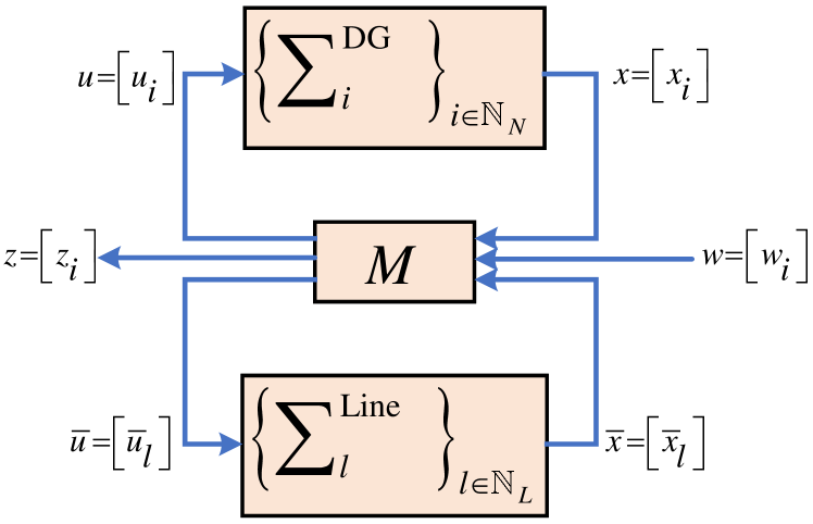
Figure 3: DC Microgrid dynamics as a networked system configuration

Let us define $u\triangleq[u_{i}]_{i}$ control input of DG $i$, $\bar{u}\triangleq[\bar{u_{l}}]_{l}$ control input of transmission line, $x\triangleq[x_{i}]_{i}$ full state of DG $i$, $w\triangleq[w_{i}]_{i}$ disturbance input, $z\triangleq[z_{i}]_{i}$ output performance, and $\bar{x}\triangleq[\bar{x}_{l}]_{l}$ full state of line $i$. Assume there is no constant power load ($P_{Li}=0$) as specified in Eq. (17). As a result, the closed-loop feedback linearization of the DC MG subsystem will be accomplished.

$$\dot{x_{i}}=(A_{i}+B_{i}K_{io})x_{i}+u_{i}(t)=g_{i}(x_{i})+u_{i}$$ (28)

where

$$u_{i}=\begin{bmatrix}-\frac{\bar{I}_{Li}}{C_{ti}}\\ 0\\ -V_{ri}\end{bmatrix}\\ +\begin{bmatrix}-\frac{1}{C_{ti}}\sum B_{il}I_{l}\\ 0\\ 0\end{bmatrix}+\begin{bmatrix}0\\ \frac{1}{L_{ti}}\sum f_{ij}\\ 0\end{bmatrix}$$ (29)

So, we have:

$$u_{i}=w_{i}+\sum_{l\in\mathbb{N}_{L}}\bar{C}_{il}\bar{x}_{l}+\sum_{j\in\mathbb{N}_{N}}K_{ij}x_{j}=w+\bar{C}\bar{x}+Kx_{j}$$ (30)

where $\bar{C}_{il}=\begin{bmatrix}-\frac{B_{il}}{C_{ti}}&0&0\end{bmatrix}^{\top}$, and

$$K_{ij}=\frac{1}{L_{ti}}\begin{bmatrix}0&0&0\\ k_{ij}^{V}&k_{ij}^{I}&k_{ij}^{v}\\ 0&0&0\end{bmatrix}$$ (31)

where $\bar{C}=[\bar{C}_{il}]_{i\in\mathbb{N}_{N},l\in\mathbb{N}_{L}}$ and $K=[k_{ij}]_{i,j\in\mathbb{N}_{N}}$. On the other hand, the line dynamic of Eq. (23) can be written as:

$$\dot{x_{l}}=(A_{l}+B_{l}K_{lo})x_{l}+u_{l}(t)=\bar{g}_{l}(\bar{x}_{l})+\bar{u}_{l}$$ (32)

where $K_{lo}$ is the feedback controller for line $l$ and can be defined as follows:

$$f_{lo}(I_{l})=K_{lo}x_{l}(t),$$ (33)

such that

$$\bar{u}_{l}=\sum_{i\in\mathbb{N}_{N}}C_{il}x_{i}$$ (34)

with $C_{il}\triangleq\begin{bmatrix}\frac{B_{il}}{L_{l}}&0&0\end{bmatrix}$. So we have:

$$\bar{u}=Cx$$ (35)

where $C=[C_{il}]_{i\in\mathbb{N}_{N},l\in\mathbb{N}_{L}}$. Then, the output performance can be written as:

$$z_{i}=v_{i}=\begin{bmatrix}0&0&1\end{bmatrix}x_{i}=D$$ (36)

So we have:

$$z=Dx$$ (37)

where $D=\text{diag}(\begin{bmatrix}0&0&1\end{bmatrix})$. Now, using the above equations, we get:

$$\begin{cases}M_{ux}=K,\quad M_{u\bar{x}}=\bar{C},\quad M_{uw}=\mathbf{I}\\ M_{\bar{u}x}=C,\quad M_{\bar{u}\bar{x}}=\mathbf{0},\quad M_{\bar{u}w}=\mathbf{0}\\ M_{zx}=D,\quad M_{z\bar{x}}=\mathbf{0},\quad M_{zw}=\mathbf{0}\end{cases}$$ (38)

V Passivity-based Control

The organization of this section is as follows. The initial focus is on introducing the global controller design challenge for the networked system. Subsequently, we provide a set of essential prerequisites for the dissipativity properties of the subsystem in order to accomplish feasible and efficient global controller design. Next, we introduce the enhanced local controller design problem that ensures the relevant requirements are met. In conclusion, we provide a concise overview of the whole process for designing both local and global controllers.

V-A Global Controller Synthesis

A subsystem $\hat{\Sigma}_{i},i\in\mathbb{N}_{N}$ (28) is assumed to be $X_{i}$-EID (strictly passive; i.e., IF-OFP($\nu_{i},\rho_{i}$)) with

$$X_{i}=\begin{bmatrix}X_{i}^{11}&X_{i}^{12}\\ X_{i}^{21}&X_{i}^{22}\end{bmatrix}\triangleq\begin{bmatrix}-\nu_{i}\mathbf{I}&\frac{1}{2}\mathbf{I}\\ \frac{1}{2}\mathbf{I}&-\rho_{i}\mathbf{I}\end{bmatrix}$$ (39)

where $\rho_{i}$ and $\nu_{i}$ are passivity indices that are fixed and known. The interconnection matrix $M$ (38) and its block $M_{ux}=[K_{ij}]_{i,j\in\mathbb{N}_{N}}$ will be synthesized by applying these subsystem EID properties to Prop. 3. By synthesizing the matrices $[K_{ij}]_{i,j\in\mathbb{N}_{N}}$, we can uniquely compute the controller gains $\{k_{ij}:i,j\in\mathbb{N}_{N}\}$ (31).
We need the overall DC MG dynamics (i.e., the networked system $\tilde{\Sigma}$) in Fig. (3) to be $L_{2}$-stable (Y-dissipative) based on Prop 2. The following theorem formulates the centralized controller synthesis problem as an LMI problem that can be solved using standard convex optimization toolboxes.

Theorem 1.

The closed-loop dynamics of the DG illustrated in Fig. 3 can be finite-gain $L_{2}$-stable with some $L_{2}$-gain $\gamma$ (where $\tilde{\gamma}\triangleq\gamma^{2}<\bar{\gamma}$) from the disturbance input $w(t)$ to the performance output $z(t)$. The interconnection matrix block $M_{ux}=[K_{ij}]_{i,j\in\mathbb{N}_{N}}$ (38), which is synthesized via the solution of the LMI problem, is utilized to achieve this.

$$\min_{Q,\gamma,\{p_{i}:i\in\mathbb{N}_{N}\}}\sum_{i,j\in\mathbb{N}_{N}}c_{ij}\|Q_{ij}\|_{1}+c_{0}\tilde{\gamma},\ 0<\tilde{\gamma}<\bar{\gamma}$$ (40a)

$$\mbox{Sub. to: }p_{i}>0,\forall i\in\mathbb{N}_{N},\ \bar{p}_{i}>0,\forall i\in\mathbb{N}_{L};l\in\mathbb{N}_{L},$$

$$\mbox{and LMI condition in Eq.}\ \eqref{globalcontrollertheorem}\ \$$

In this context, the structure of $Q\triangleq[Q_{ij}]_{i,j\in\mathbb{N}_{N}}$ is identical to that of $M_{\eta e}$, where $c_{0}>0$ is a predetermined constant. Other parameters are defined as $\textbf{X}^{12}\triangleq\text{diag}(-\frac{1}{2\nu_{i}}\mathbf{I}:i\in\mathbb{N}_{N})$, $\textbf{X}^{21}\triangleq(\textbf{X}^{12})^{\top}$, $\bar{\textbf{X}}^{12}\triangleq\text{diag}(-\frac{1}{2\bar{\nu}_{l}}\mathbf{I}:l\in\mathbb{N}_{L})$ $\bar{\textbf{X}}^{21}\triangleq(\bar{\textbf{X}}^{12})^{\top}$, $\textbf{X}_{p}^{11}\triangleq\text{diag}(-p_{i}\nu_{i}\mathbf{I}:i\in\mathbb{N}_{N})$, $\textbf{X}_{p}^{22}\triangleq\text{diag}(-p_{i}\rho_{i}\mathbf{I}:i\in\mathbb{N}_{N})$, $\bar{\textbf{X}}_{\bar{p}}^{11}\triangleq\text{diag}(-\bar{p}_{l}\bar{\nu}_{l}\mathbf{I}:l\in\mathbb{N}_{L})$, $\bar{\textbf{X}}_{\bar{p}}^{22}\triangleq\text{diag}(-\bar{p}_{l}\bar{\rho}_{l}\mathbf{I}:l\in\mathbb{N}_{L})$, and $M_{\eta e}\triangleq(\textbf{X}_{p}^{11})^{-1}Q$.

Proof.

By applying the networked system dissipativity properties examined in Prop. 2 and the subsystem dissipativity properties assumed in (39) to the interconnection topology synthesis result given in Prop. 3 yields the proof. ∎

$$\begin{bmatrix}\textbf{X}_{p}^{11}&\mathbf{0}&\mathbf{0}&Q&\textbf{X}_{p}^{11}\bar{C}&\textbf{X}_{p}^{11}\\ \mathbf{0}&\bar{\textbf{X}}_{\bar{p}}^{11}&\mathbf{0}&\bar{\textbf{X}}_{\bar{p}}^{11}C&\mathbf{0}&\mathbf{0}\\ \mathbf{0}&\mathbf{0}&\mathbf{I}&D&\mathbf{0}&\mathbf{0}\\ Q^{\top}&C^{\top}\bar{\textbf{X}}_{\bar{p}}^{11}&D^{\top}&-Q^{\top}\textbf{X}^{12}-\textbf{X}^{21}Q-\textbf{X}_{p}^{22}&-\textbf{X}^{21}\textbf{X}_{p}^{11}\bar{C}-C^{\top}\bar{\textbf{X}}_{\bar{p}}^{11}\bar{\textbf{X}}^{12}&-\textbf{X}^{21}\textbf{X}_{p}^{11}\\ \bar{C}^{\top}\textbf{X}_{p}^{11}&\mathbf{0}&\mathbf{0}&-\bar{C}^{\top}\textbf{X}_{p}^{11}\textbf{X}^{12}-\bar{\textbf{X}}^{21}\bar{\textbf{X}}_{\bar{p}}^{11}C&-\bar{\textbf{X}}_{\bar{p}}^{22}&\mathbf{0}\\ \textbf{X}_{p}^{11}&\mathbf{0}&\mathbf{0}&-\textbf{X}_{p}^{11}\textbf{X}^{12}&\mathbf{0}&\tilde{\gamma}\mathbf{I}\end{bmatrix}>0$$ (41)

V-B Necessary Conditions on Subsystem Passivity Indices

Lemma 1.

It is necessary for the main LMI condition (41) in Th. (1) to hold that, for each subsystem $\hat{\Sigma}_{i},i\in\mathbb{N}_{N}$ (28), $\hat{\Sigma}_{l},l\in\mathbb{N}_{L}$ (32) the passivity indices $\nu_{i}$, $\nu_{l}$ and $\rho_{i}$, $\rho_{l}$ (39) (let $\tilde{\rho}_{i}\triangleq\frac{1}{\rho_{i}}$) are such that the LMI problem:

Find: $$\nu_{i},\ \bar{\nu}_{l},\ \tilde{\rho}_{i},\ \bar{\rho}_{l},\ \tilde{\gamma}_{i},$$ (42a)

Sub. to: $$-\frac{\tilde{\gamma}_{i}}{p_{i}}<\nu_{i}<0,$$ (42b)

$$0<\tilde{\rho_{i}}<p_{i},$$ (42c)

$$0<\tilde{\rho_{i}}<\frac{4\tilde{\gamma}_{i}}{p_{i}},$$ (42d)

$$\bar{\rho}_{l}>\frac{p_{i}\nu_{i}}{\bar{p}_{l}C_{ti}^{2}},$$ (42e)

$$\bar{\rho}_{l}>\frac{\tilde{\rho}_{i}}{p_{i}\bar{p}_{l}}(\frac{p_{i}}{2C_{ti}}-\frac{\bar{p}_{l}}{2L_{l}})^{2},$$ (42f)

$$\bar{\nu}_{l}<-\frac{p_{i}\rho_{i}L_{l}^{2}}{\bar{p}_{l}}<0,$$ (42g)

is feasible.

Proof.

It is expected that for any $i\in\mathbb{N}_{N}$, there will exist scalars $0<\tilde{\gamma}_{i}<\tilde{\gamma}$ if the global controller theorem (41) holds. In other words, (41) is true if and only if there exists $\tilde{\Gamma}\triangleq\text{diag}(\tilde{\gamma}_{i}\mathbf{I}:i\in\mathbb{N}_{N})$ where $0<\tilde{\Gamma}<\tilde{\gamma}\mathbf{I}$.

To ensure the validity of the LMI condition in (41), it is possible to identify the following set of necessary conditions by examining particular sub-block matrices of the block matrix in (41):

$$\textbf{X}_{p}^{11}>0,\ \bar{\textbf{X}}_{\bar{p}}^{11}>0$$ (43a)

$$-Q^{\top}\textbf{X}^{12}-\textbf{X}^{21}Q-\textbf{X}_{p}^{22}>0$$ (43b)

$$\bar{\textbf{X}}_{\bar{p}}^{22}>0,$$ (43c)

$$\begin{bmatrix}\textbf{X}_{p}^{11}&\textbf{X}_{p}^{11}\\ \textbf{X}_{p}^{11}&\tilde{\Gamma}\end{bmatrix}>0,$$ (43d)

$$\begin{bmatrix}\mathbf{I}&D\\ D^{\top}&-Q^{\top}\textbf{X}^{12}-\textbf{X}^{21}Q-\textbf{X}_{p}^{22}\end{bmatrix}>0,$$ (43e)

$$\begin{bmatrix}-Q^{\top}\textbf{X}^{12}-\textbf{X}^{21}Q-\textbf{X}_{p}^{22}&-\textbf{X}^{21}\textbf{X}_{p}^{11}\\ -\textbf{X}_{p}^{11}\textbf{X}^{12}&\tilde{\Gamma}\end{bmatrix}>0,$$ (43f)

$$\begin{bmatrix}\textbf{X}_{p}^{11}&\textbf{X}_{p}^{11}\bar{C}\\ \bar{C}^{\top}\textbf{X}_{p}^{11}&-\textbf{X}_{p}^{22}\end{bmatrix}>0,$$ (43g)

$$\begin{bmatrix}-Q^{\top}\textbf{X}^{12}-\textbf{X}^{21}Q-\textbf{X}_{p}^{22}&-\textbf{X}^{21}\textbf{X}_{p}^{11}\bar{C}-C^{\top}\bar{\textbf{X}}_{\bar{p}}^{11}\bar{\textbf{X}}^{12}\\ -\bar{C}^{\top}\textbf{X}_{p}^{11}\textbf{X}^{12}-\bar{\textbf{X}}^{12}\bar{\textbf{X}}_{\bar{p}}^{11}C&-\bar{\textbf{X}}_{\bar{p}}^{22}\end{bmatrix}>0,$$ (43h)

$$\begin{bmatrix}\bar{\textbf{X}}_{\bar{p}}^{11}&\bar{\textbf{X}}_{\bar{p}}^{11}C\\ C^{\top}\bar{\textbf{X}}_{\bar{p}}^{11}&-Q^{\top}\textbf{X}^{12}-\textbf{X}^{21}Q-\textbf{X}_{p}^{22}\end{bmatrix}>0,$$ (43i)

A required condition for (43a) is:

$$\mbox{\eqref{Eq:Lm:CodesignConditionsStep2_1}}\iff-p_{i}\nu_{i}>0\iff\nu_{i}<0,\forall i\in\mathbb{N}_{N}.$$ (44)

$$\mbox{\eqref{Eq:Lm:CodesignConditionsStep2_1}}\iff-\bar{p}_{l}\bar{\nu}_{l}>0\iff\bar{\nu}_{l}<0,\forall l\in\mathbb{N}_{L}.$$ (45)

A necessary condition for (43b) can be obtained by considering the diagonal elements of the matrix and using the structure of the matrix $Q$. Note that each $Q_{ii}$ block has zeros in its diagonal for any $i\in\mathbb{N}_{N}$.

$$\mbox{\eqref{Eq:Lm:CodesignConditionsStep2_2}}\implies \ -Q_{ii}^{\top}(-\frac{1}{2\nu_{i}}\mathbf{I})-(-\frac{1}{2\nu_{i}}\mathbf{I})Q_{ii}-(-p_{i}\rho_{i}\mathbf{I})>0$$

$$\implies \ p_{i}\rho_{i}>0\iff\rho_{i}>0,\forall i\in\mathbb{N}_{N}.$$ (46)

$$\mbox{\eqref{Eq:Lm:CodesignConditionsStep2_3}}\iff -(-\bar{p}_{l}\bar{\rho}_{l}\mathbf{I})>0$$

$$\implies \bar{p}_{l}\bar{\rho}_{l}>0\iff\bar{\rho}_{l}>0,\forall l\in\mathbb{N}_{L}.$$ (47)

To derive the necessary conditions for (43d)-(43i), we can obtain:

$$\mbox{\eqref{Eq:Lm:CodesignConditionsStep2_4}}\iff \ \begin{bmatrix}-p_{i}\nu_{i}&-p_{i}\nu_{i}\\ -p_{i}\nu_{i}&\tilde{\gamma}_{i}\end{bmatrix}>0\iff-p_{i}\nu_{i}(\tilde{\gamma}_{i}+p_{i}\nu_{i})>0$$

$$\iff \ \nu_{i}>-\frac{\tilde{\gamma}_{i}}{p_{i}},\forall i\in\mathbb{N}_{N};$$ (48)

$$\mbox{\eqref{Eq:Lm:CodesignConditionsStep2_5}}\implies \ \begin{bmatrix}1&1\\ 1&p_{i}\rho_{i}\end{bmatrix}>0\iff\rho_{i}>\frac{1}{p_{i}},\forall i\in\mathbb{N}_{N};$$ (49)

$$\mbox{\eqref{Eq:Lm:CodesignConditionsStep2_6}}\implies \ \begin{bmatrix}p_{i}\rho_{i}&-\frac{1}{2}p_{i}\\ -\frac{1}{2}p_{i}&\tilde{\gamma}_{i}\end{bmatrix}>0\iff p_{i}(\rho_{i}\tilde{\gamma}_{i}-\frac{1}{4}p_{i})>0$$

$$\iff \ \rho_{i}>\frac{p_{i}}{4\tilde{\gamma}_{i}},\forall i\in\mathbb{N}_{N}.$$ (50)

$$\mbox{\eqref{Eq:Lm:CodesignConditionsStep2_7}}\implies \ \begin{bmatrix}-p_{i}\nu_{i}&-p_{i}\nu_{i}\frac{B_{il}}{C_{ti}}\\ -\frac{B_{il}}{C_{ti}}p_{i}\nu_{i}&\bar{p}_{l}\bar{\rho}_{l}\end{bmatrix}>0$$

$$\iff (-p_{i}\nu_{i}\bar{p}_{l}\bar{\rho}_{l})-(p_{i}^{2}\nu_{i}^{2}\frac{B_{il}^{2}}{C_{ti}^{2}})>0$$

$$\iff \bar{\rho}_{l}>\frac{p_{i}\nu_{i}}{\bar{p}_{l}C_{ti}^{2}},\forall i\in\mathbb{N}_{N};l\in\mathbb{N}_{L}.$$ (51)

$$\mbox{\eqref{Eq:Lm:CodesignConditionsStep2_8}}\implies \ \begin{bmatrix}-p_{i}\rho_{i}&-\frac{p_{i}\nu_{i}B_{il}}{2C_{ti}}-\frac{B_{il}\bar{p}_{l}}{L_{l}}\\ -\frac{p_{i}\nu_{i}B_{il}}{2C_{ti}}-\frac{B_{il}\bar{p}_{l}}{L_{l}}&\bar{p}_{l}\bar{\rho}_{l}\end{bmatrix}>0$$

$$\iff p_{i}\rho_{i}\bar{p}_{l}\bar{\rho}_{l}-(\frac{p_{i}}{2C_{ti}}-\frac{\bar{p}_{l}}{2L_{l}})^{2}>0$$

$$\iff \bar{\rho}_{l}>\frac{\tilde{\rho}_{i}}{p_{i}\bar{p}_{l}}(\frac{p_{i}}{2C_{ti}}-\frac{\bar{p}_{l}}{2L_{l}})^{2},\forall i\in\mathbb{N}_{N};l\in\mathbb{N}_{L}.$$ (52)

$$\mbox{\eqref{Eq:Lm:CodesignConditionsStep2_9}}\implies \ \begin{bmatrix}-\bar{p}_{l}\bar{\nu}_{l}&-\bar{p}_{l}\bar{\nu}_{l}\frac{B_{il}}{L_{l}}\\ -\bar{p}_{l}\bar{\nu}_{l}\frac{B_{il}}{L_{l}}&-\frac{B_{il}}{L_{l}}\bar{p}_{l}\bar{\nu}_{l}\end{bmatrix}>0$$

$$\iff (-\bar{p}_{l}\bar{\nu}_{l}p_{i}\rho_{i})-(\frac{\bar{p}_{l}\bar{\nu}_{l}B_{il}}{L_{l}})^{2}>0,$$

$$\iff \bar{\nu}_{l}<-\frac{p_{i}\rho_{i}L_{l}^{2}}{\bar{p}_{l}},\forall i\in\mathbb{N}_{N};l\in\mathbb{N}_{L}.$$ (53)

In conclusion, we can obtain the set of LMI problems (42) (each in variables $\nu_{i},\nu_{l},\ \tilde{\rho}_{i},\ \bar{\rho}_{l},\ \tilde{\gamma}_{i}$, for any $i\in\mathbb{N}_{N};l\in\mathbb{N}_{L}$) by carrying out the following: (1) compiling the requisite conditions as shown in (44)-(53) and (2) employing the change of variables $\tilde{\rho}_{i}\triangleq\frac{1}{\rho_{i}},\forall i\in\mathbb{N}_{N}$, and (3) recognizing each $p_{i},i\in\mathbb{N}_{N}$ and $\bar{p}_{l},l\in\mathbb{N}_{L}$ as a predefined positive scalar parameter. ∎

V-C Local Controller Synthesis

Theorem 2.

The local controller gains $K_{io}$ (26) should be made by solving the LMI problem for each DG $\Sigma_{i},i\in\mathbb{N}_{N}$ and a certain scalar parameter $p_{i}>0$. This will create the closed-loop dynamic $\Sigma_{i}$ (28)) IF-OFP($\nu_{i},\rho_{i}$) (as assumed in (39) while also meeting the conditions set out in Lm. 1.

Find: $$\ \tilde{K}_{io},\ P_{i},\ \nu_{i},\ \tilde{\rho}_{i},\ \tilde{\gamma}_{i},$$ (54)

Sub. to: $$\ P_{i}>0,$$

$$\ \begin{bmatrix}\tilde{\rho}_{i}\mathbf{I}&P_{i}&\mathbf{0}\\ P_{i}&-\mathcal{H}(AP_{i}+B\tilde{K}_{io})&-I+\frac{1}{2}P_{i}\\ \mathbf{0}&-I+\frac{1}{2}P_{i}&-\nu_{i}\mathbf{I}\end{bmatrix}>0,$$

Sub. to: $$\ -\frac{\tilde{\gamma}_{i}}{p_{i}}<\nu_{i}<0,$$

$$\ 0<\tilde{\rho_{i}}<\min\left\{p_{i},\frac{4\tilde{\gamma}_{i}}{p_{i}}\right\}$$

$$\bar{\rho}_{l}>\frac{p_{i}\nu_{i}}{\bar{p}_{l}C_{ti}^{2}},$$

$$\bar{\rho}_{l}>\frac{\tilde{\rho}_{i}}{p_{i}\bar{p}_{l}}(\frac{p_{i}}{2C_{ti}}-\frac{\bar{p}_{l}}{2L_{l}})^{2},$$

$$\bar{\nu}_{l}<-\frac{p_{i}\rho_{i}L_{l}^{2}}{\bar{p}_{l}}<0,$$

where $\rho_{i}\triangleq\frac{1}{\tilde{\rho}_{i}}$ and $K_{io}\triangleq\tilde{K}_{io}P_{i}^{-1}$.

We design the local controller for lines as follows:

Theorem 3.

The local controller gains $K_{lo}$ (33) should be made by solving the LMI problem for each line $\Sigma_{l},l\in\mathbb{N}_{L}$ and a certain scalar parameter $\bar{p}_{l}>0$. This will create the closed-loop dynamic $\Sigma_{l}$ (32) IF-OFP($\bar{\nu}_{l},\bar{\rho}_{l}$) while also meeting the conditions set out in Lm. 1.

Find: $$\ \tilde{K}_{lo},\ P_{l},\ \bar{\nu}_{l},\ \bar{\rho}_{l},$$ (55)

Sub. to: $$\ P_{l}>0,$$

$$\ \begin{bmatrix}\rho_{l}\mathbf{I}&P_{l}&\mathbf{0}\\ P_{l}&-\mathcal{H}(AP_{l}+B\tilde{K}_{lo})&-I+\frac{1}{2}P_{l}\\ \mathbf{0}&-I+\frac{1}{2}P_{l}&-\bar{\nu}_{l}\mathbf{I}\end{bmatrix}>0,$$

Sub. to: $$\bar{\rho}_{l}>\frac{p_{i}\nu_{i}}{\bar{p}_{l}C_{ti}^{2}},$$

$$\bar{\rho}_{l}>\frac{\tilde{\rho}_{i}}{p_{i}\bar{p}_{l}}(\frac{p_{i}}{2C_{ti}}-\frac{\bar{p}_{l}}{2L_{l}})^{2},$$

$$\bar{\nu}_{l}<-\frac{p_{i}\rho_{i}L_{l}^{2}}{\bar{p}_{l}}<0,$$

where $K_{io}\triangleq\tilde{K}_{lo}P_{l}^{-1}$.

The proof follows from: (1) considering the DG dynamic model identified in (28) and line dynamic model identified in (32) then applying the LMI-based controller synthesis technique so as to enforce the subsystem passivity indices assumed in (39), and then (2) enforcing the necessary conditions on subsystem passivity indices identified in Lm. 1 so as to ensure a feasible and effective global controller design at (41).

To conclude this section, we summarize the three main steps necessary for designing local controllers, global controllers and communication topology (in a centralized manner, for the considered microgrid) as:
Step 1. Choose proper parameters $p_{i}>0,\forall i\in\mathcal{N}_{N}$ and $\bar{p}_{l}>0,\forall l\in\mathcal{N}_{L}$;
Step 2. Synthesize local controller using Th. (2) and Th. (3).
Step 3. Synthesize global controller using Th. (1).

VI Conclusion

In this paper, we propose a passivity-based co-design controller for DC microgrids where the DGs and lines are considered as two individual subsystems that are linked through the interconnection matrix. By using a distributed control approach, the output voltages can be restored to the nominal value while optimizing the communication topology. Furthermore, the proposed controller is capable of handling the plug-and-play feature, where the DGs and the correspondence line can join or leave the microgrid without compromising the stability of the system since the controller is composed incrementally without the need to re-design the remaining DGs and lines.

References

- [1] P. Nahata, R. Soloperto, M. Tucci, A. Martinelli, and G. Ferrari-Trecate, “A passivity-based approach to voltage stabilization in dc microgrids with zip loads,” Automatica, vol. 113, p. 108770, 2020.
- [2] M. Tucci, S. Riverso, and G. Ferrari-Trecate, “Line-independent plug-and-play controllers for voltage stabilization in dc microgrids,” IEEE Transactions on Control Systems Technology, vol. 26, no. 3, pp. 1115–1123, 2017.
- [3] E. Agarwal, S. Sivaranjani, V. Gupta, and P. J. Antsaklis, “Distributed synthesis of local controllers for networked systems with arbitrary interconnection topologies,” IEEE Transactions on Automatic Control, vol. 66, no. 2, pp. 683–698, 2020.
- [4] M. Cucuzzella, K. C. Kosaraju, and J. M. Scherpen, “Distributed passivity-based control of dc microgrids,” in 2019 American Control Conference (ACC). IEEE, 2019, pp. 652–657.
- [5] Y.-C. Jeung, D.-C. Lee, T. Dragičević, and F. Blaabjerg, “Design of passivity-based damping controller for suppressing power oscillations in dc microgrids,” IEEE Transactions on Power Electronics, vol. 36, no. 4, pp. 4016–4028, 2020.
- [6] M. Afkar, R. Gavagsaz-Ghoachani, M. Phattanasak, and S. Pierfederici, “Decentralized passivity-based control of two distributed generation units in dc microgrids,” in 2023 8th International Conference on Technology and Energy Management (ICTEM). IEEE, 2023, pp. 1–5.
- [7] S. Samanta, S. Mishra, T. Ghosh et al., “Control of dc microgrid using interconnection and damping assignment passivity based control method,” in 2022 IEEE 7th International conference for Convergence in Technology (I2CT). IEEE, 2022, pp. 1–6.
- [8] J. Loranca-Coutiño, J. C. Mayo-Maldonado, G. Escobar, T. M. Maupong, J. E. Valdez-Resendiz, and J. C. Rosas-Caro, “Data-driven passivity-based control design for modular dc microgrids,” IEEE Transactions on Industrial Electronics, vol. 69, no. 3, pp. 2545–2556, 2021.
- [9] M. A. Hassan and Y. He, “Constant power load stabilization in dc microgrid systems using passivity-based control with nonlinear disturbance observer,” IEEE Access, vol. 8, pp. 92 393–92 406, 2020.
- [10] M. A. Hassan, E.-p. Li, X. Li, T. Li, C. Duan, and S. Chi, “Adaptive passivity-based control of dc–dc buck power converter with constant power load in dc microgrid systems,” IEEE Journal of Emerging and Selected Topics in Power Electronics, vol. 7, no. 3, pp. 2029–2040, 2018.
- [11] M. A. Hassan, M. Sadiq, C.-L. Su et al., “Adaptive passivity-based control for bidirectional dc-dc power converter supplying constant power loads in dc shipboard microgrids,” in 2021 IEEE International Future Energy Electronics Conference (IFEEC). IEEE, 2021, pp. 1–6.
- [12] M. Abdolahi, J. Adabi, and S. Y. M. Mousavi, “An adaptive extended kalman filter with passivity-based control for dc-dc converter in dc microgrids supplying constant power loads,” IEEE Transactions on Industrial Electronics, 2023.
- [13] J. E. Machado and J. Schiffer, “A passivity-inspired design of power-voltage droop controllers for dc microgrids with electrical network dynamics,” in 2020 59th IEEE Conference on Decision and Control (CDC). IEEE, 2020, pp. 3060–3065.
- [14] J. Yu, J. Yu, Y. Wang, Y. Cao, X. Lu, and D. Zhao, “Passivity-based active stabilization for dc microgrid applications,” CSEE Journal of Power and Energy Systems, vol. 4, no. 1, pp. 29–38, 2018.
- [15] M. Arcak, “Compositional design and verification of large-scale systems using dissipativity theory: Determining stability and performance from subsystem properties and interconnection structures,” IEEE Control Systems Magazine, vol. 42, no. 2, pp. 51–62, 2022.
- [16] S. Welikala, Z. Song, P. J. Antsaklis, and H. Lin, “Dissipativity-based decentralized co-design of distributed controllers and communication topologies for vehicular platoons,” arXiv preprint arXiv:2312.06472, 2023.
- [17] S. Welikala, H. Lin, and P. J. Antsaklis, “Non-linear networked systems analysis and synthesis using dissipativity theory,” in 2023 American Control Conference (ACC). IEEE, 2023, pp. 2951–2956.
- [18] F. Dorfler and F. Bullo, “Kron reduction of graphs with applications to electrical networks,” IEEE Transactions on Circuits and Systems I: Regular Papers, vol. 60, no. 1, pp. 150–163, 2012.