Block-Map-Based Localization in Large-Scale Environment

Abstract

Accurate localization is an essential technology for the flexible navigation of robots in large-scale environments. Both SLAM-based and map-based localization will increase the computing load due to the increase in map size, which will affect downstream tasks such as robot navigation and services. To this end, we propose a localization system based on Block Maps (BMs) to reduce the computational load caused by maintaining large-scale maps. Firstly, we introduce a method for generating block maps and the corresponding switching strategies, ensuring that the robot can estimate the state in large-scale environments by loading local map information. Secondly, global localization according to Branch-and-Bound Search (BBS) in the 3D map is introduced to provide the initial pose. Finally, a graph-based optimization method is adopted with a dynamic sliding window that determines what factors are being marginalized whether a robot is exposed to a BM or switching to another one, which maintains the accuracy and efficiency of pose tracking. Comparison experiments are performed on publicly available large-scale datasets. Results show that the proposed method can track the robot pose even though the map scale reaches more than 6 kilometers, while efficient and accurate localization is still guaranteed on NCLT[6] and M2DGR[35]. Codes and data will be publicly available on https://github.com/YixFeng/block_localization.

I INTRODUCTION

For large-scale robotic automation in GPS-denied environments, such as indoor industrial environments, and underground mining, efficient and precise localization is a fundamental capability required by most autonomous mobile systems.

GNSS/INS systems suffer from the signal block in urban scenarios[14], which makes the localization result unreliable. The maturation of the 3D map construction achieved through the offline processing of LiDAR or camera data is evident. Particularly prominent within the domain of robotic systems operating within predetermined memory limitation, the employment of LiDAR/visual odometry for the purpose of localization introduces a salient challenge arising from the proclivity for error accumulation. This characteristic engenders deviations in the proficient execution of tasks entrusted to robotic entities. In light of this, an alternate strategy of heightened efficacy emerges, characterized by the utilization of the meticulously organized map, engendered via offline methodologies, as a steadfast and dependable modality of localization. Consequently, the adoption of map-based localization assumes paramount importance for autonomous mobile systems with distinct operational objectives such as remote delivery and mobile operations, among others. Using dense maps [9] is usually more accurate but suffers from high computational time. The use of feature maps[18] decreases the computational time and makes the localization task more suitable for real-time application. Even so, the increase in the scale of the map aggravates the performance overhead and the search domain uncertainty of the registration process, which leads to a decrease in the real-time and accuracy of robot localization.

Various approaches based on camera[33] and LiDAR[5] are proposed for Map-based localization. During which, LiDAR has been widely used for environment perception thanks to their accurate range measurements. Besides, as a result of accurate short-term motion constraints at high frequency, IMU is adopted for compensating deficiencies of LiDAR. Popular solutions for Lidar-Inertial based state estimation can be divided into two categories: filtering-based and optimization-based approaches. Filtering-based approaches infer the most likely state from available measurements and uncertainties, while optimization-based approaches try to minimize reprojection error to find the optimal states. However, the filter-based algorithm assumes Markovianity, which is a fundamental constraint limiting its performance, and global batch optimization cannot guarantee real-time performance[1].

Figure 1: Dividing a large-scale map into multiple block maps has the potential to enable robots to utilize limited resources to achieve arbitrary scale navigation and service tasks. Consequently, the utilization of block map-based localization becomes indispensable.

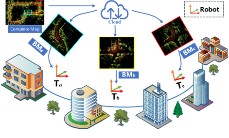
To address these limitations, we propose a BM generation and maintenance method and the corresponding BM-based localization system 1. We employ keyframe stitching instead of segmenting the entire global map. This approach ensures spatial continuity between block maps through the overlap of keyframes, thereby preventing the loss of correlation information between the robot’s laser point cloud and the map when transiting between maps. Consequently, given a coarse pose of the robot, BBS is utilized on the pyramid of a given BM to get the initial pose. On top of this, for the trade-off of accuracy and efficiency in pose tracking, we propose a factor graph-based optimization method with the dynamic sliding window that maintains different factors in cases of the same BM and switching BM.

In summary, our contributions are as follows:

• A BM-based localization system in a large-scale environment is proposed for the first time.

• A BM generation method and corresponding switching strategy is proposed which maintains the spatial continuity of adjacent BMs.

• A factor graph-based optimization method with the dynamic sliding window based on BMs is proposed to achieve accurate and reliable state estimation.

• We achieve the best performance on publicly available large-scale datasets.

II Related Work

Building a 3D map of an unknown environment is crucial for map-based localization, which provides necessary information for path planning. Due to the dense and accurate depth measurements of environments, 3D LiDAR has emerged as an essential sensor for robots. The cartographer[16] make the laser fan project onto the horizontal plane using an IMU, which is applicable to relatively flat ground scenes. LOAM[37] introduces planes and edges as features to achieve low-drift and low-computational complexity. Inspired by LOAM, there have been multiple variations of LOAM that enhance its performance. By incorporating IMU data through tight coupling for the state estimation[32, 21, 23], SLAM systems naturally become more precise and flexible. Iterative closest points (ICP), Normal Distribution Transform (NDT) and their variances are also utilized as state estimation methods for odometry of LiDAR SLAM[10, 36, 12]. NDT reduces the computational time with respect to ICP approaches, while keeping the accuracy. None of the above methods implements the solution of dividing a large-scale map into several block maps.

Given the map generated by LiDAR SLAM, we often distinguish localization problem between global localization and pose tracking [28]. For global localization, Monte Carlo localization[29] is a popular framework, which uses a particle filter to estimate the robot’s pose and is widely used in robot localization systems[9, 25]. This filtering methodology should be more robust to local minima because the particles should ideally come to a consensus through additional measurements — though this is dependent on random sampling and can make no time-based optimality guarantees. As one of the most successful algorithms for global optimization problem[2, 15], BBS has been widely used for localization in autonomous driving[8, 31].

High-rate IMU measurements can effectively compensate for the motion distortion in a LiDAR scan. To achieve robust state estimation in challenging situations, LiDAR fused with IMU has become prevailing in the process of map-based pose tracking. Levinson[20] adopt the particle filter to combine multiple observations for state estimation. Zhen[38] uses the Error State Kalman Filter (ESKF) for sensor fusion and is combined with a Gaussian Particle Filter (GPF) for measurements update. Iterated Error State Kalman Filter (IESKF) [23] is designed to correct the estimated state recursively by generating new feature correspondences in each iteration, which enables robust and efficient navigation for ground vehicles in feature-less scenes. Lie Group has been introduced to define the state and reduce the linearization error in Invariant Extended Kalman Filter (Invariant EKF)[26], Iterative Error State Kalman Filter[27] and Invariant Unscented Kalman Filter (Invariant UKF)[3]. Nevertheless, the Markov assumptions limit the performance of filter-based state estimation, while the factor graph optimization (FGO) presents a smoothing state estimation framework for flexible sensor fusion[22, 11]. As the FGO with high accuracy is computationally expensive, localization with sliding window factor graphs[11, 30] are proposed to provide highly accurate pose estimates in real-time.

III Method

Figure 2: Overview of our Block-Map-Based Localization which consists of four main modules: a block maps generation module, a pose initialization module, a map retrieval server module and a pose tracking module.

III-A System Overview

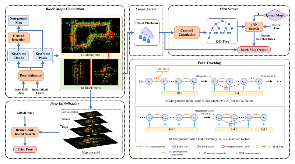
As Fig.2 shows, based on the poses $\mathbf{T}^{W_{\textrm{off}}}_{\textrm{off},m}$ obtained from offline graph-based SLAM[7], we opt for keyframe fusion as opposed to segmenting the entire global map. This approach ensures spatial continuity between block maps by leveraging the overlap among keyframes, thereby preventing the loss of correlation information between the robot’s laser point cloud and the map during map transitions. Additionally, we calculate the map centroid and establish a KD-Tree structure to maintain the map retrieval repository. Subsequently, we emulate cloud storage using ROS Services to store the maps in the cloud. The retrieval through BBS on three-dimensional maps at different resolutions enables the robot to achieve coarse-to-fine global localization. To ensure robustness in the robot’s pose tracking for localization, we employ sliding window-based factor graph optimization to ensure that the robot leverages a sufficient amount of historical information. When switching BMs, due to the loss of a substantial amount of prior map information, we dynamically adjust the sliding window, and aim to mitigate the interference caused by irrelevant historical data.

III-B Block Maps Generation

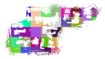
In the Block-Map-Based localization method, maintaining spatial continuity in robotic observations during BM transitions is of paramount importance to ensure smooth estimates and stability. To address this, our proposed methodology focuses on the deployment of keyframe-based integration to build BMs, instead of the more traditional method of partitioning a comprehensive map into isolated BMs, as Fig.3b, which neglects the relational integrity of map information between contiguous BMs. The intricate procedure is elucidated in Algorithm III-B.

  Algorithm 1 Block Maps (BMs) Generation Method

 

0:  LiDAR raw points in all $k$ scans $\{^{L}\mathbf{p}_{i}\}_{k}$;      Highly precise poses obtained from offline SLAM $\mathbf{T}^{W_{\textrm{off}}}_{\textrm{off},m}$;      Extrinsic parameters $\mathbf{T}^{L}_{\textrm{off}}$;     Block map size $\mathcal{S}$.

0:  The block maps $\{^{W_{l}}\mathbf{BM}_{j}\}$.

1:  Block maps count $\mathcal{C}=0$;

2:  for all pointcloud ${}^{L}\mathbf{p}_{i}$ in $\{^{L}\mathbf{p}_{i}\}_{k}$ do

3:     Find the closest pose $\mathbf{T}^{W_{\textrm{off}}}_{\textrm{off}}$ to the pointcloud timestamp;

4:     Transform LiDAR points via ${}^{\textrm{off}}\mathbf{p}_{i}=({\mathbf{T}^{L}_{\textrm{off}}})^{-1}{{}^{L}\mathbf{p}_{i}}$;

5:     if it is the first pointcloud then

6:        Record the translation part of the corresponding pose as $\widehat{\mathbf{t}}^{W_{\textrm{off}}}_{\textrm{off}}$;

7:        Create a new ${}^{W_{l}}\widehat{\mathbf{BM}}$ for temporary storage;

8:     end if

9:     $\mathbf{t}^{W_{\textrm{off}}}_{\textrm{off}}$ denotes the translation part of $\mathbf{T}^{W_{\textrm{off}}}_{\textrm{off}}$;

10:     if $Euclidean\_dist(\widehat{\mathbf{t}}^{W_{\textrm{off}}}_{\textrm{off}},\mathbf{t}^{W_{\textrm{off}}}_{\textrm{off}})\leq\mathcal{S}$ then

11:        ${}^{W_{l}}\widehat{\mathbf{BM}}={{}^{W_{l}}\widehat{\mathbf{BM}}}\cup{\mathbf{T}^{L}_{\textrm{off}}}{\mathbf{T}^{W_{\textrm{off}}}_{\textrm{off}}}{{}^{\textrm{off}}\mathbf{p}_{i}}$;

12:     else

13:        $\widehat{\mathbf{t}}^{W_{\textrm{off}}}_{\textrm{off}}={\mathbf{t}}^{W_{\textrm{off}}}_{\textrm{off}}$;

14:        if $\mathcal{C}$ is equal to $0$ or $1$ then

15:           Store ${}^{W_{l}}\widehat{\mathbf{BM}}$ with its count as ${}^{W_{l}}\mathbf{BM}_{j}$;

16:           Compute its centroid point ${}^{W_{l}}\mathbf{p}_{c}$ and build a KD-Tree using all centroids;

17:           $\mathcal{C}=\mathcal{C}+1$;

18:        else

19:           Compute the centroid of ${}^{W_{l}}\widehat{\mathbf{BM}}$;

20:           Find its nearest neighbor in KD-Tree and save the minimum distance $\mathbf{d}$ and index $\mathbf{n}$;

21:           if $\mathbf{d}\geq 0.5\mathcal{S}$ then

22:              Redo lines 15 to 17;

23:           else if $0.1\mathcal{S}<\mathbf{d}<0.5\mathcal{S}$ then

24:              ${}^{W_{l}}\mathbf{BM}_{\mathbf{n}}={{}^{W_{l}}\mathbf{BM}_{\mathbf{n}}}\cup{{}^{W_{l}}\widehat{\mathbf{BM}}}$;

25:              Renew the centroid and update the KD-Tree;

26:           end if

27:        end if

28:        Clear the ${}^{W_{l}}\widehat{\mathbf{BM}}$.

29:     end if

30:  end for

 

In our approach, as the robot frame in offline SLAM denoted as ${}^{\textrm{off}}$ is different from the lidar frame, we leverage the extrinsics $\mathbf{T}^{L}_{\textrm{off}}$ to reproject the points into the frame ${}^{\textrm{off}}$ and build the BMs by $\mathbf{T}^{W_{\textrm{off}}}_{\textrm{off}}$. To filter out excessively overlapping BMs while remaining more map information, we compute the centroids of the BMs to maintain a KD-Tree. When a new candidate BM is completed, we use its centroid to search for the nearest BM, and if the distance $\mathbf{d}$ satisfies $0.1\mathcal{S}<\mathbf{d}<0.5\mathcal{S}$, we merge these two BMs to maintain an appropriate map overlap.

This strategy effectively capitalizes on the overlapping segments among keyframes, thereby ensuring a seamless scan-to-map alignment during the map transition process.

III-C Pose Initialization

(a) Ours

(b) Gao’s[13]

Figure 3: The result comparison of different block maps separation methods. Our method considers the overlap between adjacent block maps, and the robot will not lose prior information when switching maps at the boundary.

Initializing the pose of robots is the beginning of the whole system. The initial pose gives the first prior for the factor graph to stabilize the non-linear optimization process. Inspired by [17], we build up a pyramid of different resolution maps for searching. In the searching step, we start from the minimum resolution map and recursively iterate from the highest score branch to the lowest score branch. To reduce the computing cost of BBS, we simplified the search process by giving an adapted initial score $\mathbf{S}_{0}$.

We are interested in finding the accurate $\epsilon$ in the initial block map, as shown in the Eq.(1):

$$\epsilon^{*}=\mathop{\arg\min}_{\epsilon\in\mathbb{L}}\text{M}(\mathbf{T}_{\epsilon}\mathbf{h}_{k}),$$ (1)

where $\epsilon^{*}$ is the optimizing pose in the block maps. $\mathbf{T}_{\epsilon}$ is pose $\epsilon$ represented in Lie Group. $\text{M}(\cdot)$ is a measurement function to get the score of current pose $\epsilon$ in 2D block map planers just as [17].

Firstly, a map pyramid $\mathbf{P}_{m}$ from level $0$ to level $N$ is built, and each level is represented as $\mathbb{L}_{i}\in\mathbf{P}_{m}(i=0,1,\cdots,N)$. The resolution of $\mathbb{L}_{i}$ is half that of $\mathbb{L}_{i-1}$. Secondly, we choose the angular $\delta_{\theta}$ and the linear $r$ step sizes in searching. For each $\mathbb{L}_{i}(i=0,1,\cdots,N)$, create a search window $\mathcal{W}^{i}$ in $\mathbb{L}_{i}$.

$$w^{i}_{x}=\left\lceil\frac{\mathbf{W}^{i}_{x}}{r}\right\rceil,w^{i}_{y}=\left\lceil\frac{\mathbf{W}^{i}_{y}}{r}\right\rceil,w^{i}_{\theta}=\left\lceil\frac{\mathbf{W}^{i}_{\theta}}{\delta_{\theta}}\right\rceil,$$ (2)

$$\overline{\mathcal{W}}^{i}=\{-w^{i}_{x},\cdots,w^{i}_{x}\}\times\{-w^{i}_{y},\cdots,w^{i}_{y}\}\times\{-w^{i}_{\theta},\cdots,w^{i}_{\theta}\},$$ (3)

$$\mathcal{W}^{i}=\{\epsilon_{0}+(rj_{x},rj_{y},rj_{\theta})\ |\ (rj_{x},rj_{y},rj_{\theta})\in\overline{\mathcal{W}}^{i}\}.$$ (4)

Finally, adaptively select a base score for branch and bound search.

III-D Pose Tracking

III-D1 Problem Formulation

We propose our graph-based optimization framework with a changeable sliding window size. In our case, we define a set of poses $\bm{x}=\{\bm{x}_{t_{s}},\cdots,\bm{x}_{t_{e}}\}$ and observations $\bm{z}$, where $t_{s}$ and $t_{e}$ are the first and last pose in the sliding window respectively. We seek to estimate the most likely states of the robot $\bm{x}$ over a set of measurements $\bm{z}$ from various sensors inside the current sliding window. This problem can be formulated as a maximum a posteriori (MAP) problem:

$$\bm{x}^{*}=\mathop{\arg\max}_{\bm{x}}P(\bm{z}\ |\ \bm{x})P(\bm{x}),$$ (5)

Assuming the noise follows the Gaussian distribution and is independent, Eq.(5) can be rewritten as a sum of minimum cost functions:

$$\bm{x}^{*}=\mathop{\arg\min}_{\bm{x}}\sum_{k}\bm{e}_{k}(\bm{x},\bm{z}_{k})^{\top}\bm{\Omega}_{k}\bm{e}_{k}(\bm{x},\bm{z}_{k}),$$ (6)

$\bm{e}_{k}(\bm{x},\bm{z}_{k})$ denotes the cost functions between robot state vector $\bm{x}$ and measurements $\bm{z}_{k}$, and $\bm{\Omega}_{k}$ is the corresponding information matrices. To be specific, we introduce three types of error functions and a prior from sliding window marginalization:

$$\bm{x}^{*}=\mathop{\arg\min}_{\bm{x}} \sum_{k}\bm{e}^{\textrm{odm}}(\bm{x},\bm{z}_{k}^{\textrm{odm}})^{\top}\bm{\Omega}_{k}^{\textrm{odm}}\bm{e}^{\textrm{odm}}(\bm{x},\bm{z}_{k}^{\textrm{odm}})$$ (7)

$$+ \sum_{k}\bm{e}^{\textrm{map}}(\bm{x},\bm{z}_{k}^{\textrm{map}})^{\top}\bm{\Omega}_{k}^{\textrm{map}}\bm{e}^{\textrm{map}}(\bm{x},\bm{z}_{k}^{\textrm{map}})$$

$$+ \sum_{k}\bm{e}^{\textrm{imu}}(\bm{x},\bm{z}_{k}^{\textrm{imu}})^{\top}\bm{\Omega}_{k}^{\textrm{imu}}\bm{e}^{\textrm{imu}}(\bm{x},\bm{z}_{k}^{\textrm{imu}})$$

$$+ \mathcal{F}^{\textrm{marg}}(\bm{x}).$$

We differentiate between error functions by superscripts, ${}^{\textrm{map}}$ for NDT matching errors, ${}^{\textrm{odm}}$ for odometry errors, and ${}^{\textrm{imu}}$ for IMU preintegration measurements between subsequent poses. Additionally, $\mathcal{F}^{\textrm{marg}}(\bm{x})$ stands for the prior information that derives from marginalized measurements outside the sliding window.

III-D2 Point Deskewing

Due to the particular mechanism of the rotating 3D lidar, the raw scan received, $\mathcal{P}_{k}$, is distorted when moving at a fast speed. To cope with this issue, we use the steady-speed motion model from previous poses to predict lidar translation and obtain the rotation from IMU forward propagation. Denote the lidar pose of the k-th sweep as $\mathbf{T}_{k}$ and the transformation between two consecutive frames $k-1$ to $k$ can be represented by:

$$\xi^{k-1}_{k}=\log(\mathbf{T}_{k-2}^{-1}\mathbf{T}_{k-1})\in\mathfrak{se}(3),$$ (8)

Then, we use the timestamp $t\in(t_{k},t_{k^{\prime}}]$ of each point to interpolate the lidar motion, where $t_{k}$ is the beginning of the k-th sweep and $t_{k^{\prime}}$ is the end:

$$\mathbf{T}_{k}(t)=\mathbf{T}_{k-1}\exp(\frac{t-t_{k}}{t_{k^{\prime}}-t_{k}}{\xi^{k-1}_{k}}),$$ (9)

The raw points $\mathcal{P}_{k}$ can be corrected into the starting pose of the sweep:

$$\widetilde{\mathcal{P}}_{k}=\{\mathbf{T}_{k}(t)\mathbf{p}_{k}\ |\ \mathbf{p}_{k}\in\mathcal{P}_{k}\}.$$ (10)

III-D3 Dynamic Sliding Window

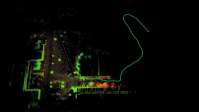
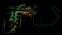
In this section, we introduce our marginalization strategy with changeable sliding window size. The number of active keyframes in the current sliding window depends on two BM-related cases shown in the pose tracking module of Fig.2. In the first case, when the robot navigates in a single BM, we keep a maximum of $N_{a}=20$ keyframes and marginalize the old set of variables. By linearizing these factors, the linear system becomes:

$$\begin{bmatrix}\mathbf{H}_{\alpha\alpha}&\mathbf{H}_{\alpha\beta}\\ \mathbf{H}_{\beta\alpha}&\mathbf{H}_{\beta\beta}\end{bmatrix}\begin{bmatrix}\bm{x}_{\alpha}\\ \bm{x}_{\beta}\end{bmatrix}=\begin{bmatrix}\mathbf{b}_{\alpha}\\ \mathbf{b}_{\beta}\end{bmatrix},$$ (11)

where $\beta$ denotes the set of variables that have to be marginalized, and all variables dependent on them are regarded as $\alpha$. Then, we apply the Schur complement, which yields a new linear system $\widehat{\mathbf{H}_{\alpha\alpha}}\bm{x}_{\alpha}=\widehat{\mathbf{b}_{\alpha}}$ with:

$$\widehat{\mathbf{H}_{\alpha\alpha}}=\mathbf{H}_{\alpha\alpha}-\mathbf{H}_{\alpha\beta}\mathbf{H}_{\beta\beta}^{-1}\mathbf{H}_{\beta\alpha},$$ (12)

$$\widehat{\mathbf{b}_{\alpha}}=\mathbf{b}_{\alpha}-\mathbf{H}_{\alpha\beta}\mathbf{H}_{\beta\beta}^{-1}\mathbf{b}_{\beta}.$$ (13)

This strategy creates a marginalization factor connecting all variables related to the factors removed.

In another case, the robot traverses the boundary of BMs which means the system has to retrieve a new BM for the source of scan-to-map alignment. Towards the goal of retaining enough but not redundant historical information, we only reserve $N_{r}=5$ keyframes in the current sliding window when BM switching and all factors before will be marginalized as a prior. The design of reserved factors corresponds to the information involved in the overlapping zone of adjacent BMs. It aims to estimate a smooth trajectory while switching the map instead of violent fluctuations.

(a)

(b)

(c)

(d)

Figure 4: Subfigures (a) to (d) show smooth transition and the localization path passing through 4 consecutive block maps on nclt_2. Our switching strategy is able to maintain spatial continuity with good performance.

IV Experiment and Results

IV-A Dataset

We evaluate our method on two publicly available datasets, NCLT[7] and M2DGR[35]. To demonstrate our method’s superior performance in large-scale environments, we select the longest sequence from these two datasets, as shown in Table IV. Specifically, the North Campus Long-Term (NCLT) dataset, collected at the University of Michigan’s North Campus, is a large-scale, long-term autonomy dataset for unmanned ground vehicles. It includes a 10 Hz Velodyne HDL-32E LiDAR and a 100 Hz Microstrain 3DM-GX3-45 IMU for the LIO system. While the same area is repeatedly explored, each sequence features diverse paths and encompasses both outdoor and indoor scenes. We choose five sequences from the NCLT dataset, with two of them extending beyond 6 kilometers in length.

The M2DGR dataset comprises large-scale sequences for ground robots, equipped with a comprehensive sensor suite, including a Velodyne VLP-32C LiDAR and a 150 Hz 9-axis IMU for the LIO system. It records trajectories in challenging situations commonly encountered in practical applications, such as entering elevators and navigating in complete darkness. We select the two longest sequences from the M2DGR dataset to validate the universality of our approach.

IV-B Pose Initialization

To evaluate the accuracy of initial pose estimation, we measured the translation error and the time cost of algorithms compared with various methods including [4, 17, 34]. Given that both [4] and [34] consume considerable time initializing map descriptors using the FPFH process (exceeding one hour), rendering them unsuitable for robot global localization. Our approach, compared to the traditional Branch and Bound Search (BBS), employs a greedy strategy to reduce potentially ineffective searches, thereby accelerating localization efficiency. As delineated in Table I, within a search range of 40$\times$40 meters, our method achieves localization times of less than 1 second, ensuring computational precision while striking a balance between computational efficiency and accuracy.

TABLE I: Global localization evaluation

Method	Translational Error (m)	Time (s)
FPFH+RANSAC[4]	0.26	4036.36
FPFH+Teaser[34]	0.16	3935.50
BBS[17]	5.00	9.82
Ours	0.05	0.87

IV-C Pose Tracking Evaluation

In this section, we implement all experiments on an Intel i9-12700K CPU with 64GB of RAM for fairness. We conducted a rigorous evaluation of two state-of-the-art (SOTA) incremental SLAM-based state estimation algorithms [24, 32] and two map-based localization algorithms Hdl-Localization [19] and Fastlio-Loc, which is adapted from FAST-LIO2, loaded the global map once and then utilize the Iterated Extended Kalman Filter (IEKF) for state estimation. Additionally, to ensure a consistent and equitable comparison with Hdl-Localization, and taking into account the pertinence of control variables, we uniformly employed the NDT registration algorithm predicated on “DIRECT1”. This particular approach entails searching the 1-neighbor voxel to compute the gradient of the matching score. The results of our analysis are delineated in Table II. We evaluate the Root Mean Square Error (RMSE) for two distinct trajectory patterns: the “xyz” mode (trans_part) and the “xyzrpy” mode (full). Through an in-depth quantitative evaluation, it is evident that our method outperforms other methods on the long-distance NCLT dataset and consistently demonstrates stable performance across all datasets. This superior performance and stability can largely be attributed to our deployment of a sliding window based on factor graph optimization for state estimation and block maps generation and transition strategy, which exhibits robustness in both outdoor and indoor scenes. This strategy circumvents the inherent instability of state estimations stemming from the Markov assumption, which is commonly associated with filter-based methodologies.

TABLE II: absolute trajectory errors (rmse, meters) comparison of state-of-the-arts

Method	nclt_1		nclt_2		nclt_3		nclt_4		nclt_5		m2dgr_1		m2dgr_2
	part	full	part	full	part	full	part	full	part	full	part	full	part	full
LIO-SAM	$\times$	$\times$	$\times$	$\times$	$\times$	$\times$	2.1779	3.5690	$\times$	$\times$	1.4513	3.1022	6.3035	6.8771
FAST-LIO2	1.8562	3.3829	1.8400	3.3740	1.8456	3.3816	1.4103	3.1604	2.4028	3.7110	0.4199	2.7773	2.8482	3.9557
Hdl-Loc	$\times$	$\times$	$\times$	$\times$	$\times$	$\times$	$\times$	$\times$	0.5023	2.8725	$\times$	$\times$	$\times$	$\times$
Fastlio-Loc	$\times$	$\times$	3.0193	4.1371	0.1795	2.8340	0.1973	2.8352	$\times$	$\times$	0.1457	2.7524	0.1302	2.7513
Ours	0.9736	2.9904	0.1983	2.8345	0.1854	2.8337	0.1832	2.8336	0.1529	2.8316	0.2336	2.7561	0.2206	2.7570

• $\times$ denotes that the system totally failed.

TABLE III: Average Time consumption of state update when using global maps and block maps respectively (ms)

Method	nclt_1	nclt_2	nclt_3	nclt_4	nclt_5	m2dgr_1	m2dgr_2
Fastlio-Loc	10.25*	11.12	10.57	12.33	12.45*	14.75	11.68
Hdl-Loc	8.55*	8.75*	17.39*	$\times$	19.67	20.52*	$\times$
Ours w/ Global Map	27.35	35.92	31.15	37.25	29.11	24.66	24.43
Ours w/ Block Map	15.25	14.28	18.16	22.25	20.61	14.64	11.17

• $*$ denotes that the system failed in the middle and we calculate the average time before each failure.

• $\times$ denotes that the system totally failed.

IV-D Efficiency Evaluation

The method of map-blocking proposed by Gao [13] lacks a mechanism for maintaining a map library, rendering it unsuitable for our evaluation of localization performance. Consequently, our comparison is confined to the efficacy of existing map-based localization techniques relative to our own, specifically when employing both global and block maps. As shown in Table III, the algorithm we employ with the block map is notably faster compared to the one using the entire global map especially when the map is particularly large. In the sequence nclt_2, we have increased the speed by 150%. However, it is worth noting that as the map continues to grow, our time consumption advantages will become more conspicuous. Additionally, the algorithm based on filtering exhibits an obvious advantage in terms of speed but lacks stability and accuracy. Our block map algorithm is quite close to theirs in terms of speed and performs more robustly in large-scale environments.

TABLE IV: details of all the sequences

Abbreviation	Name	Duration (min:sec)	Distance (km)
nclt_1	20120115	111:46	4.01
nclt_2	20120122	87:19	6.36
nclt_3	20120202	98:37	6.45
nclt_4	20120429	43:17	1.86
nclt_5	20120511	84:32	3.13
m2dgr_1	street_01	17:08	0.75
m2dgr_2	street_02	20:27	1.48

V Conclusion

In this paper, we have proposed a localization system based on block maps in large-scale environments. To enhance the robustness of robot localization, we have incorporated a factor graph optimization method based on a dynamic sliding window, effectively leveraging more historical information to mitigate the uncertainties associated with the Markov assumption, aligning with our block map switching strategy. Finally, we validated the superiority of our approach on publicly available large-scale datasets. In future work, we intend to further enhance this system. We aim to ensure that the robot can achieve real-time and accurate global localization in any position and in highly dynamic environments within the framework of block maps. Additionally, we plan to detect real-time changes in the environment and update the block maps accordingly, catering to applications such as logistics and food delivery robots.

References

- [1] Timothy D Barfoot. State estimation for robotics. Cambridge University Press, 2017.
- [2] Thomas M Breuel. Implementation techniques for geometric branch-and-bound matching methods. Computer Vision and Image Understanding, 90(3):258–294, 2003.
- [3] Martin Brossard, Silvere Bonnabel, and Jean-Philippe Condomines. Unscented kalman filtering on lie groups. In 2017 IEEE/RSJ International Conference on Intelligent Robots and Systems (IROS), pages 2485–2491. IEEE, 2017.
- [4] Anders Glent Buch, Dirk Kraft, Joni-Kristian Kamarainen, Henrik Gordon Petersen, and Norbert Krüger. Pose estimation using local structure-specific shape and appearance context. In 2013 IEEE International Conference on Robotics and Automation, pages 2080–2087, 2013.
- [5] Fernando Caballero and Luis Merino. Dll: Direct lidar localization. a map-based localization approach for aerial robots. In 2021 IEEE/RSJ International Conference on Intelligent Robots and Systems (IROS), pages 5491–5498. IEEE, 2021.
- [6] Nicholas Carlevaris-Bianco, Arash K. Ushani, and Ryan M. Eustice. University of Michigan North Campus long-term vision and lidar dataset. International Journal of Robotics Research, 35(9):1023–1035, 2015.
- [7] Nicholas Carlevaris-Bianco, Arash K Ushani, and Ryan M Eustice. University of michigan north campus long-term vision and lidar dataset. The International Journal of Robotics Research, 35(9):1023–1035, 2016.
- [8] Guang Chen, Fan Lu, Zhijun Li, Yinlong Liu, Jinhu Dong, Junqiao Zhao, Junwei Yu, and Alois Knoll. Pole-curb fusion based robust and efficient autonomous vehicle localization system with branch-and-bound global optimization and local grid map method. IEEE Transactions on Vehicular Technology, 70(11):11283–11294, 2021.
- [9] Xieyuanli Chen, Ignacio Vizzo, Thomas Läbe, Jens Behley, and Cyrill Stachniss. Range image-based lidar localization for autonomous vehicles. In 2021 IEEE International Conference on Robotics and Automation (ICRA), pages 5802–5808. IEEE, 2021.
- [10] Pierre Dellenbach, Jean-Emmanuel Deschaud, Bastien Jacquet, and François Goulette. Ct-icp: Real-time elastic lidar odometry with loop closure. In 2022 International Conference on Robotics and Automation (ICRA), pages 5580–5586. IEEE, 2022.
- [11] Wendong Ding, Shenhua Hou, Hang Gao, Guowei Wan, and Shiyu Song. Lidar inertial odometry aided robust lidar localization system in changing city scenes. In 2020 IEEE International Conference on Robotics and Automation (ICRA), pages 4322–4328. IEEE, 2020.
- [12] Erik Einhorn and Horst-Michael Gross. Generic ndt mapping in dynamic environments and its application for lifelong slam. Robotics and Autonomous Systems, 69:28–39, 2015.
- [13] Xiang Gao. Slam in autonomous driving book. https://github.com/gaoxiang12/slam_in_autonomous_driving, 2023.
- [14] Yanlei Gu, Li-Ta Hsu, and Shunsuke Kamijo. Gnss/onboard inertial sensor integration with the aid of 3-d building map for lane-level vehicle self-localization in urban canyon. IEEE Transactions on Vehicular Technology, 65(6):4274–4287, 2015.
- [15] Richard I Hartley and Fredrik Kahl. Global optimization through rotation space search. International Journal of Computer Vision, 82(1):64–79, 2009.
- [16] Wolfgang Hess, Damon Kohler, Holger Rapp, and Daniel Andor. Real-time loop closure in 2d lidar slam. In 2016 IEEE international conference on robotics and automation (ICRA), pages 1271–1278. IEEE, 2016.
- [17] Wolfgang Hess, Damon Kohler, Holger Rapp, and Daniel Andor. Real-time loop closure in 2d lidar slam. In 2016 IEEE International Conference on Robotics and Automation (ICRA), pages 1271–1278, 2016.
- [18] Kichun Jo, Yongwoo Jo, Jae Kyu Suhr, Ho Gi Jung, and Myoungho Sunwoo. Precise localization of an autonomous car based on probabilistic noise models of road surface marker features using multiple cameras. IEEE Transactions on Intelligent Transportation Systems, 16(6):3377–3392, 2015.
- [19] Kenji Koide, Jun Miura, and Emanuele Menegatti. A portable three-dimensional lidar-based system for long-term and wide-area people behavior measurement. International Journal of Advanced Robotic Systems, 16(2):1729881419841532, 2019.
- [20] Jesse Levinson, Michael Montemerlo, and Sebastian Thrun. Map-based precision vehicle localization in urban environments. In Robotics: science and systems, volume 4, page 1. Atlanta, GA, USA, 2007.
- [21] Kailai Li, Meng Li, and Uwe D Hanebeck. Towards high-performance solid-state-lidar-inertial odometry and mapping. IEEE Robotics and Automation Letters, 6(3):5167–5174, 2021.
- [22] Julian Nubert, Shehryar Khattak, and Marco Hutter. Graph-based multi-sensor fusion for consistent localization of autonomous construction robots. In IEEE International Conference on Robotics and Automation (ICRA). IEEE, 2022.
- [23] Chao Qin, Haoyang Ye, Christian E Pranata, Jun Han, Shuyang Zhang, and Ming Liu. Lins: A lidar-inertial state estimator for robust and efficient navigation. In 2020 IEEE international conference on robotics and automation (ICRA), pages 8899–8906. IEEE, 2020.
- [24] Tixiao Shan, Brendan Englot, Drew Meyers, Wei Wang, Carlo Ratti, and Rus Daniela. Lio-sam: Tightly-coupled lidar inertial odometry via smoothing and mapping. In IEEE/RSJ International Conference on Intelligent Robots and Systems (IROS), pages 5135–5142. IEEE, 2020.
- [25] Li Sun, Daniel Adolfsson, Martin Magnusson, Henrik Andreasson, Ingmar Posner, and Tom Duckett. Localising faster: Efficient and precise lidar-based robot localisation in large-scale environments. In 2020 IEEE International Conference on Robotics and Automation (ICRA), pages 4386–4392, 2020.
- [26] Zhongxing Tao, Jianru Xue, Di Wang, Gengxin Li, and Jianwu Fang. An adaptive invariant ekf for map-aided localization using 3d point cloud. IEEE Transactions on Intelligent Transportation Systems, pages 1–14, 2022.
- [27] Zhongxing Tao, Jianru Xue, Di Wang, Gengxin Li, and Jianwu Fang. An adaptive invariant ekf for map-aided localization using 3d point cloud. IEEE Transactions on Intelligent Transportation Systems, 2022.
- [28] S. Thrun, W. Burgard, and D. Fox. Probabilistic Robotics (Intelligent Robotics and Autonomous Agents). Probabilistic Robotics (Intelligent Robotics and Autonomous Agents), 2005.
- [29] Sebastian Thrun, Dieter Fox, Wolfram Burgard, and Frank Dellaert. Robust monte carlo localization for mobile robots. Artificial intelligence, 128(1-2):99–141, 2001.
- [30] Daniel Wilbers, Lars Rumberg, and Cyrill Stachniss. Approximating marginalization with sparse global priors for sliding window slam-graphs. In 2019 Third IEEE International Conference on Robotic Computing (IRC), pages 25–31. IEEE, 2019.
- [31] Ryan W Wolcott and Ryan M Eustice. Fast lidar localization using multiresolution gaussian mixture maps. In 2015 IEEE international conference on robotics and automation (ICRA), pages 2814–2821. IEEE, 2015.
- [32] Wei Xu, Yixi Cai, Dongjiao He, Jiarong Lin, and Fu Zhang. Fast-lio2: Fast direct lidar-inertial odometry. IEEE Transactions on Robotics, 2022.
- [33] Yuquan Xu, Vijay John, Seiichi Mita, Hossein Tehrani, Kazuhisa Ishimaru, and Sakiko Nishino. 3d point cloud map based vehicle localization using stereo camera. In 2017 IEEE intelligent vehicles symposium (IV), pages 487–492. IEEE, 2017.
- [34] Heng Yang, Jingnan Shi, and Luca Carlone. Teaser: Fast and certifiable point cloud registration. IEEE Transactions on Robotics, 37(2):314–333, 2021.
- [35] Jie Yin, Ang Li, Tao Li, Wenxian Yu, and Danping Zou. M2dgr: A multi-sensor and multi-scenario slam dataset for ground robots. IEEE Robotics and Automation Letters, pages 1–1, 2021.
- [36] Masashi Yokozuka, Kenji Koide, Shuji Oishi, and Atsuhiko Banno. Litamin2: Ultra light lidar-based slam using geometric approximation applied with kl-divergence. In 2021 IEEE International Conference on Robotics and Automation (ICRA), pages 11619–11625. IEEE, 2021.
- [37] Ji Zhang and Sanjiv Singh. Loam: Lidar odometry and mapping in real-time. In Robotics: Science and Systems, volume 2, pages 1–9. Berkeley, CA, 2014.
- [38] Weikun Zhen, Sam Zeng, and Sebastian Soberer. Robust localization and localizability estimation with a rotating laser scanner. In 2017 IEEE international conference on robotics and automation (ICRA), pages 6240–6245. IEEE, 2017.