Naïve Bayes Classifiers and One-hot Encoding of Categorical Variables
Abstract
This paper investigates the consequences of encoding a -valued categorical variable incorrectly as bits via one-hot encoding, when using a Naïve Bayes classifier. This gives rise to a product-of-Bernoullis (PoB) assumption, rather than the correct categorical Naïve Bayes classifier. The differences between the two classifiers are analysed mathematically and experimentally. In our experiments using probability vectors drawn from a Dirichlet distribution, the two classifiers are found to agree on the maximum a posteriori class label for most cases, although the posterior probabilities are usually greater for the PoB case.
Consider a Naïve Bayes classifier that uses a categorical variable in order to predict a class label . An example of such a variable is eye colour, which may take on values brown, gray, blue, green etc. Suppose that can take on different values, coded as . The correct way to make use of this variable in a Naïve Bayes classifier is to estimate for for each possible value of ; see, e.g., Murphy, (2022, sec. 9.3). However, sometimes the categorical variable may be recoded as bits in a one-hot encoding scheme (see, e.g., Murphy, 2022, sec. 1.5.3.1), also known as “dummy variables” in the statistics literature. For example, this is a common input encoding for use with neural networks. If these bits are naïvely treated as independent Bernoulli variables, then the classification probabilities will not be correctly computed under the Naïve Bayes model. (Clearly the bits are not independent, as if one is on, all the rest are off).111 Note also that there are possible states of bits, but only of these are one-hot codes.
In scikit-learn (Pedregosa et al.,, 2011), the sklearn.naive_bayes classifier will work correctly if the OrdinalEncoder is used to encode categorical variables, but not if the OneHotEncoder is used for them. And, for example, the fastNaiveBayes package (Skogholt,, 2020, p. 4) “will convert non numeric columns to one hot encoded features to use with the Bernoulli event model”, i.e. not the correct behaviour for categorical variables. But it does recognize categorical variables if they are coded as integers.
Let be denoted by , and the one-hot encoding of be denoted by . Let denote , the marginal probability of the th bit in being 1. Note that there are free parameters in due to normalization, but in . Let denote the one-hot vector with a 1 in the th position. Thus assuming that the Naïve Bayes assumption applies across these bits, we have
| (1) |
Under the correct categorical model, and assuming there is only one feature , we have that
| (2) |
where is the vector of prior probabilities over the classes.
Under the product-of-Bernoullis (PoB) assumption, we have that
| (3) |
where is the vector of prior class probabilities for this model. If there was more than one categorical input feature, there will be a factor coming from each one. But factors corresponding to true Bernoulli features, or to Gaussian models for real-valued features in a Naïve Bayes classifier would be unaffected by one-hot encoding.
If the parameters of the product-of-Bernoullis model are estimated by maximum likelihood, we will have that , and that . This is because the prior class probabilities are the same for the PoB model as for the categorical model, and the probability of the th bit in being set to 1 given is . Given this, we drop the tildes on , and factors below. The differences between eqs. 2 and 3 are now that there is an additional factor of (resp. ) in the numerator (resp. denominator) of eq. 3.
Below we first analyze as a function of its parameter vector, and then consider the consequences of the change from eq. 2 to eq. 3 on the Naïve Bayes classifier. Experiments to explore this further are shown in sec. 3. We conclude with a discussion.
1 Analysis of
In this section we suppress the dependence of on the class label, and consider a parameter vector . Thus we consider
| (4) |
subject to the constraint that and that the s are non-negative. We explore how varies as a function of for a fixed value of . lives on the simplex defined by the constraint .
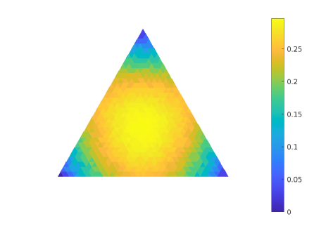
is a symmetric function of the elements of . A plot of the 4-dimensional case with is shown in Fig. 1(a). Note that the minimum values occur in the corners of the simplex (where only one of the s is non-zero), and the maximum in the centre, where they all the variables are equal.
For the general -dimensional case it is thus natural to investigate the value at the corners and centre of the simplex. At a corner we have for a single vertex , with the remaining values being 0. In this case we have .
We now use calculus to find the optimum/optima of subject to the constraint . Defining the Lagrangian , we have that
| (5) |
Setting this equal to 0 and multiplying through by , we obtain
| (6) |
where denotes the value of at the optimum (and similarly for the other variables in ). denotes the vector . Hence the optimum lies at the centre of the simplex, where for . Hence
| (7) |
and at the optimum
| (8) |
Analysis of as a function of shows that it is greater than for , with equality at (when all the other s must all be zero). To see this, at we have that , and the derivative of in the interval, so it is monotonically increasing. Hence we conclude that is bounded between its minimum value of at the corners of the simplex, and its maximum value of (as per eq. 8) obtained at the centre.
 |
 |
| (a) | (b) |
2 The effect of the factors on the Naïve Bayes classifier
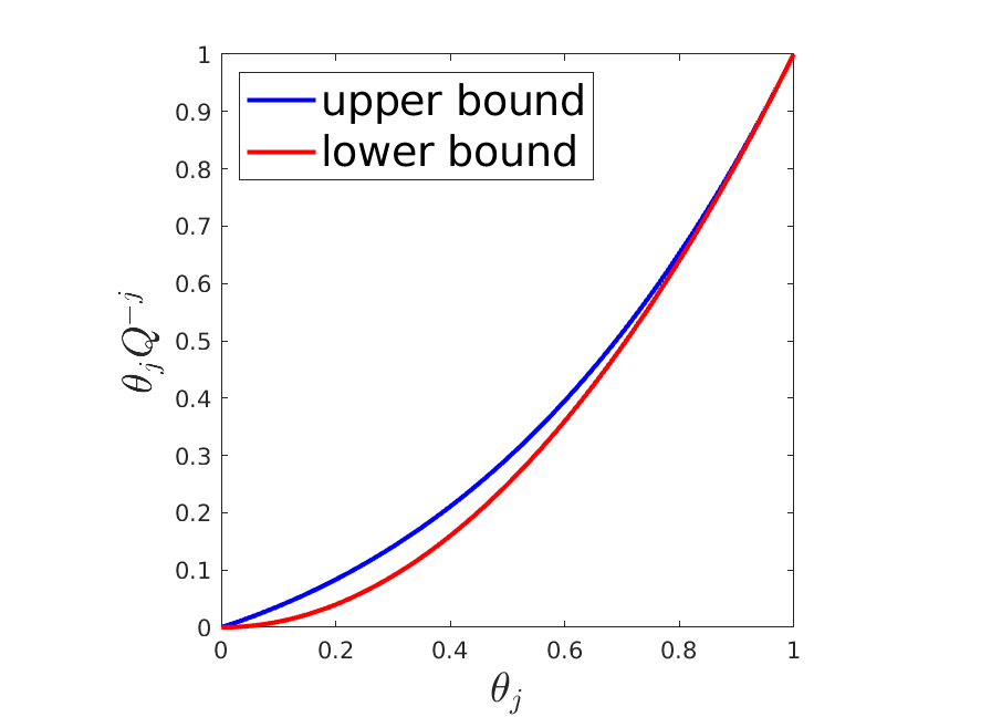
The difference between the the posterior probabilities computed under the categorical model of eq. 2 and the PoB of eq. 3 is the factors that appear in the numerator and denominator of the latter. The above analysis shows that can be bounded from above and below. Let these upper and lower bounds be denoted by and respectively, with
| (9) | ||||
| (10) |
Fig. 1(b) illustrates these bounds for . It is notable that the gap between the upper and lower bounds is small, and it is even smaller for lower .
Notice that both bounds pass through the origin and are convex functions. Elementary analysis shows that, for
| (11) |
for .
For two classes and , if , is it true that ? In general this does not hold, as if and are sufficiently close, then it could be that . However, if is sufficiently large relative to , then we will have that and thus will hold.
Applying eq. 11 to the two classes with and , we have that for both the upper and lower bounds, the ratio of the bounds is greater than . This suggests that the introduction of the factors might make the ratio more extreme than . This is backed up, on average, in the experiments in section 3.
We can make use of the upper and lower bounds to determine when the ratio is guaranteed to be more extreme than . We have that
| (12) |
So the ratio is guaranteed to be more extreme if the last term in eq. 12 is larger than 1, i.e. if
| (13) |
A similar analysis can also be used to bound from below as .
The observations above are consistent with the idea that the PoB assumption “overcounts” the evidence from the variable, relative to the correct categorical encoding.
3 Experiments
In the experiments below we generate Naïve Bayes classifiers with classes and values of . Each vector (of length ) is generated by drawing from a Dirichlet distribution , where , and similarly for each vector (of length ). gives rise to a uniform distribution across the probability simplex. would put more probability mass in the centre of the simplex, while gives rise to a sparse distribution, with “spikes” at the corners of the simplex.
 |
 |
| (a) , . | (b) , . |
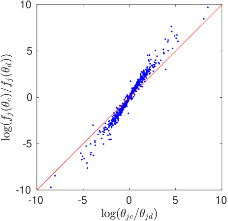
Fig. 2(a) shows a scatter plot of against . This was obtained for and sampling the vectors from the Dirichlet distribution with parameter .222The plot replicates a point at , as the order of the classes and is arbitrary. Notice that the slope of the scatterplot around is greater than 1, agreeing with the idea that, on average, the introduction of the factors makes the ratio more extreme than . There are exceptions to this (i.e. points below the diagonal for a positive log ratio) when the log ratio is not too large.
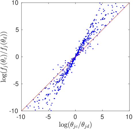
The behaviour of plot of against changes if set (maintaining ), as shown in Fig. 2(b). This value of makes the distribution sparser, so that if one value of a vector is large, the others are likely to be small. If the ratio to be large, must be large and small. This is more likely to happen for than for , and is reflected in the wider spread of points in Fig. 2(b) compared to panel (a). Another notable feature in Fig. 2(b) is the points lying on the line running from -5 to 5, corresponding to the function or . This line is not a bound, as there are some points lying above it for positive , and below it for a negative log ratio. To understand this, recall that for the ratio to be large, must be large and small. If is large, because of sparsity we would expect one of the other entries in to be near zero, and the other to be near . This would give a factor of around . Similarly if is small, we would expect one of the other entries in to be near zero, and the other to be near . This would give a factor of around . Hence we have that in this case
| (14) |
which is in agreement with the points lying on the line of slope 2 in the plot.
For scatterplots similar to Fig. 2 for and show a greater tendency for points to lie closer to the diagonal than for . As with Figures 2(a) and 2(b), the plot for exhibits a broader distribution of than for , for the same reason. Interestingly there is no obvious alignment of points on the line of slope 2 for and , in contrast to the case for .
Consequences of the transformation for the winning class.
In this paragraph we consider a two class problem. For class to be the winner under the categorical model when the observed value is , we have that or that , where denotes the other class. Let the ratio be denoted by . We now consider two cases when class is the winning class under the categorical model:
-
•
If is somewhat larger than 0, then points on the scatterplots lying to the right of the vertical line will be classified as class . Almost all of these points lie above the horizontal line , which means that they will also be classified as class , and indeed the introduction of the factors in the PoB model may well make the posterior in favour of class more extreme here.
-
•
If is somewhat less than 0, then the prior ratio is strongly in favour of class , and one can have and still have class as the winning class. However, the effect of the factors on points lying between and 0 on the x-axis of the plot tends to push them downwards, so the points in this region may have a lower posterior probability for class , or to change classification if they fall below the horizontal line .
Comparing posterior probabilities under the categorical and PoB models:
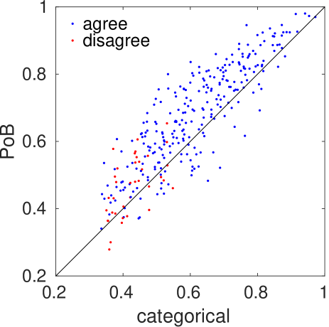
Naïve Bayes classifiers with classes were sampled times, with and states, for and . For each classifier, each observation was considered, for . Figure 3 shows a scatterplot of the maximum posterior probability under the PoB model plotted against the maximum posterior probability for the categorical model, for and . We see that the maximum probability under the PoB model is usually higher than under the exact model, in line with the observations above. This is the case 82.0% of the samples for and . Datapoints in blue show occasions where the MAP class assignment is the same under both models, while the red points mark where they disagree. Unsurprisingly, differences in MAP classification are more likely when the MAP value under the categorical model is low.
The amount of scatter around the diagonal line decreases as increases. The percentage of cases where the maximum probability under the PoB model is higher than for the exact (categorical) model are 82.0%, 72.3% and 74.7 % for and , and 78.0%, 78.1% and 76.4% respectively for .
Comparing the MAP class assignment under the categorical and PoB models:
The sampling protocol was used as in the paragraph above. For and there were 12.33% of cases where the exact and PoB classifiers disagreed over the MAP class. This reduced to 5.67% and 2.50% for and respectively. For the results were 14.33%, 7.00% and 6.30% respectively. Thus we observe fewer disagreements between the categorical and PoB classifiers as increases, and that the fraction of disagreements is somewhat higher for the sparser than for .
4 Discussion
In this paper we have investigated the differences for Naïve Bayes classification between using the exact categorical encoding model (eq. 2) and the product-of-Bernoullis model (eq. 3) arising from one-hot encoding. In our experiments with one categorical variable, these two classifiers were found to agree on the MAP class for much of the time, although the posterior probabilities were usually higher for the PoB model than the categorical model.
The analysis and experiments above were for one categorical variable . If there are multiple categorical variables which are one-hot encoded, then the effects of the transformation from to will multiply up for each variable. If the evidence from each ratio is all in the same direction then this will magnify the effect, making the class probabilities more extreme. But if the evidence of the different ratios conflicts, the effects will tend to cancel out. Also, note that if there are many features but the evidence provided by each feature is weak, we will be operating in a region towards the left-hand side of Fig. 3, where errors are more likely to occur.
Issues with the encoding of variables as identified above illustrate the importance of a data dictionary or a metadata repository giving information such as the meaning and type of each attribute in a table. If given a “bare” table we may not be aware that a categorical variable has been one-hot encoded,333It is possible to detect the linear dependence of one-hot encoded variables by linearly predicting each variable from the others, as used in variance inflation factor (VIF) analysis, see, e.g., Rawlings et al., (1989, sec. 11.3.2). leading to a mis-application of the product-of-Bernoullis model.
Acknowledgements
I thank Iain Murray for insightful comments about the role of in early draft of the manuscript.
References
- Murphy, (2022) Murphy, K. P. (2022). Probabilistic Machine Learning: An Introduction. MIT Press.
- Pedregosa et al., (2011) Pedregosa, F., Varoquaux, G., Gramfort, A., Michel, V., Thirion, B., Grisel, O., Blondel, M., Prettenhofer, P., Weiss, R., Dubourg, V., Vanderplas, J., Passos, A., Cournapeau, D., Brucher, M., Perrot, M., and Duchesnay, E. (2011). Scikit-learn: Machine learning in Python. Journal of Machine Learning Research, 12:2825–2830.
- Rawlings et al., (1989) Rawlings, J. O., Pantula, S. G., and Dickey, D. A. (1989). Applied Regression Analysis: A Research Tool. Springer-Verlag, New York, second edition.
- Skogholt, (2020) Skogholt, M. (2020). fastNaiveBayes: Extremely Fast Implementation of a Naive Bayes Classifier. R package version 2.2.1.