Magnetic phase diagram of EuPdSn2
Abstract
A magnetic phase diagram for EuPdSn2 is constructed based on magnetization, DC-susceptibility and specific heat as a function of applied field, and neutron diffraction results at zero field. The contribution of the ferromagnetic FM and antiferromagnetic AFM components to the measured magnetic susceptibility can be separated and weighted as a function of the applied field by taking the temperature dependence of the neutron counts from the FM phase at as a reference. In the magnetically ordered phase, the temperature dependence of the specific heat does not follow the mean-field prediction for the Eu2+ quantum number rather that for . This deviation and the consequent discrepancy for the entropy is discussed in the context of a non-Zeeman distribution of the eight fold ground state. Comparing the respective variations of magnetization and entropy , the thermodynamic relationship is observed for the ranges: K and T.
I Introduction
Eu2+ ions exhibit a unique property among the rare earth series that allow them to play a role in two completely different scenarios because they can mimic the magnetism of Gd3+ atoms and chemically substitute the divalent alkaline earths such as Sr and Ca. This occurs because the localization of a band electron into the Eu3+ electronic configuration: [Xe][6s25d14f6] leads to the same occupation of the orbital as that of Gd3+: [Xe][(6s5d)24f7] for Eu2+. As expected, the atomic volume of Eu2+ is considerably increased (from about 24.4Å3 to 33.4Å3) since there is an addditional electron without electronic charge compensation by another proton.
There are numerous examples of Eu2+ behaving magnetically like Gd3+, see for example [1, 2, 3, 4] and references therein. Regarding the substitution of Eu2+ in 2+ alkaline earth (e.g. Sr or Ca) sites, the number of publications has rapidly increased because of its recent applications in optical properties, e.g. to shift activated emissions towards blue spectrum [5, 6].
On the contrary, the application of the magnetic properties of Eu2+ in biological systems [7, 8] is scarce. However, the fact that magnetic circular dichroism can be used in these systems according the magnetic nature of Eu2+ provides an alternative microscopic technique that has not yet been fully exploited. Considering this potential application, it is advisable to use the study of magnetic properties of Eu2+ compounds as possible reference for future investigations of more complex and even biological systems.
The present work is devoted to the analysis of the evolution of the magnetic properties of EuPdSn2 under magnetic field with the aim of constructing a magnetic phase diagram. It is based on the field-dependent magnetic and thermal measurements [3], that takes into account the magnetic phase separation in the ground state of EuPdSn2 revealed by neutron diffraction [9] measurements at zero field.
II Magnetic properties
II.1 Magnetic Susceptility
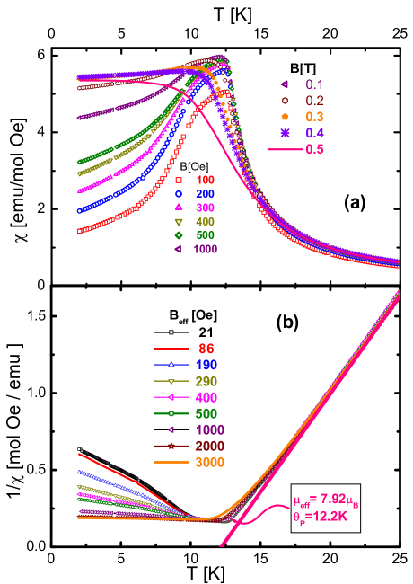
The main features reported for this compound at zero field are: an antiferromagnetic (AFM) like cusp at =12.5 K in contrast to the ferromagnetic (FM) molecular field suggested by the positive paramagnetic temperature K [3]. Coincidentally, this maximum is not a canonical AFM-cusp because it is followed at lower temperatures by a pronounced hump, whose intensity increases with field as seen in Fig. 1 a. As a result the tail increases significantly with , becoming dominant around T and showing saturation slightly above T.
It is well known that in low-field studies, the effective applied field can be affected by any residual magnetic field in the magnet when it is also used to produce intense field. This variation must be taken into account in low field measurements where the difference between nominal and effective field may become relevant. In fact, in Fig. 1a it is possible to appreciate a deviation of the measured at nominal Oe from other curves at higher field. To analyze whether this deviation is intrinsic or due to the mentioned experimental feature, we have tuned the effective values, and merged all results into a single curve as required for the pure paramagnetic regime. A further measurement, performed at nominal field Oe, was also included in Fig. 1b as the inverse susceptibility where the paramagnetic Curie-Weiss CW law is represented by a straight line whose slope corresponds to the inverse of the effective magnetic moment .
As it can be seen in the field values depicted in Fig. 1a and b, the difference between and becomes significant at low intensities. This procedure allows us to obtain more precise values for the characteristic parameters such as the Curie constant: emu K/mol, which corresponds to , and K.
II.2 Detachment of the FM and AFM components
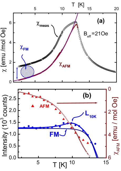
In order to check whether the anomalous maximum at , see Fig. 1a and Fig. 2a, is related to the competition between two different magnetic phases [9], one can explore the possibility of subtracting one of these contributions from the total measured signal to undress the other. Labeling both components as FM: , and AFM: , such subtraction can be expressed as , as schematized in Fig. 2a.
The key information is provided by neutron diffraction measurements [9] which shows a phase separation between FM () and AFM () at , with very different temperature dependencies, see Fig. 2b. As shown in the figure, the FM component is nearly temperature independent below 7K, but it shows a broad shoulder around K, with the full signal extrapolating to zero at K. This suggests the presence of two ferromagnetic contributions: one from the pure FM() phase and the other as a spurious (unknown) contribution [3].
The respective temperature dependencies of , can be described by two simple functions:
| (1) |
| (2) |
as depicted in the figure. The function can be associated with the ferromagnetic order parameter which is zero for , while is a Lorentzian function accounting for the broad anomaly centered at K, with a width K, being a scaling factor related to the intensity of that magnetic signal.
Since the resulting curve should be related to the AFM order parameter: , in Fig. 2b we compare (brown curve) this result with the neutron scattering counts using an: formula, with the scale factors counts/emu/molOe and and taking into account the fact that the AFM signal tends to zero when and increases monotonically with .
One can see in Fig. 2a the result of this subtraction (i.e. ) which was performed for the lowest measured field Oe. This curve can be described by the function: emu/mol Oe, which is consistent with the expectations for an anisotropic AFM system [10]. To improve the fit, a linear T contribution was added indicating the presence of a continuous distribution of magnetic excitations below 6K and a gap in the magnon spectrum K.
II.2.1 Field dependence of the FM contribution
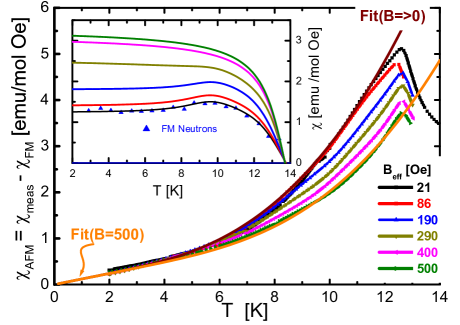
Once the values of parameters and have been determined in eqs.(1) and (2) for , the subtraction procedure can be applied for higher values with the same functions and the corresponding and parameters. The checking constraint is that the obtained data have must have the same temperature dependence as that for , represented in Fig. 2b by the AFM counts of neutron diffraction. Note that in the figure the calculated refers to the right axis with inverted growth since for .
In Fig. 3 we show these results for Oe, including the fits for (brown curve) and 500 Oe (orange curve). The only change in the fit is the enhanced gap that reaches K. While increases moderately, decreases and tends to zero around Oe. The inset of Fig. 3 collects the curves calculated using the and coefficients up to 500 Oe, showing that the contribution disappears around this field.
II.3 Magnetization
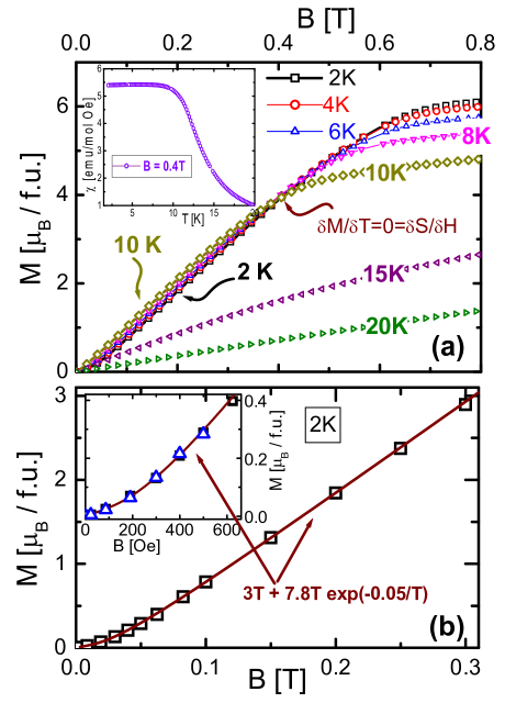
Together with the peculiar maximum at , another unusual behavior is observed in this compound. At K, the magnetization increases quite linearly up to T, see Fig. 4a. At higher fields, tends to saturate to /f.u. after undergoing a pronounced curvature above T.
Notably the isotherm shows slightly lower values than the isotherm. This peculiar feature is related to a crossing of these and intermediate isotherms ( and 8 K) at a point where . Two properties can be inferred from this zero value derivative: i) at constant field, it can be written as that means a constant value at that field, as shown in the inset of Fig. 4a for T. ii) applying the thermodynamic relationship: , this means that there is a field independent entropy collected around 10 K. This peculiarity will be discussed in the section devoted to thermal properties.
A more detailed analysis of at low field (see Fig. 4b) indicates that, after a weak (AFM-like) increase, tends to grow linearly according to a heuristic function: . A further check of the validity of the subtraction procedure used in Section B can be done by comparing the variation of the FM- coefficient (blue open triangles) obtained from the results with the direct measurement of at 2K (black squares) because is proportional to the intensity of the FM signal.
III Thermal properties
III.1 Specific Heat
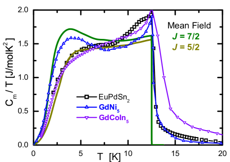
Fig. 5 shows the temperature dependence of the magnetic contribution to the specific heat of EuPdSn2 at zero magnetic field, which looks quite different from the expected for a system with in mean field approximation MFA (green curve) [11]. In order to show that such a deviation from the predicted behavior is not an isolated case, we included two Gd-based compounds that can be taken as a reference for atoms. In both cases their respective were renormalized to the of EuPdSn2. While the of GdNi5 [12] approaches the theoretical prediction, GdCoIn5 [13] behaves very similarly to EuPdSn2. Notably, the observed behavior of these two compounds is better described by the MFA for (dark yellow curve). This means that the eight-fold ground state does not split homogeneously (i.e. Zeeman like) within the ordered phase when the internal (or molecular) field increases. In all measurements, increases significantly, so that the jump in the specific heat at exceeds the prediction for a system in MFA [11]. Furthermore, in GdCoIn5 [13] the cusp at was associated with a similar cusp in thermal expansion [13], implying an unusual accumulation of entropy around this temperature.
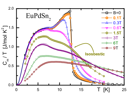
Under applied magnetic field, shows the typical variation for a FM behavior, see Fig. 6, with the exception of two nearly independent humps. While one remains practically unchanged around 6K up to T the intensity of other, which has its origin in the cusp, decreases significantly its intensity with field. One can recognize the presence of an isosbestic point where [14], that holds at least up to 1.5 T. This means that above this field, overcomes the internal field and increasingly dominates the scenario.
Fig. 6 also shows a fit of the data for T. This fit, which includes the two observed humps, is performed using two contributions based on the relation [11], where is a Brillouin function with , and the main quantum number used for the fit.
| (3) |
where and . In this case, the contribution with the maximum at K is represented by and involves levels, while the other: , describes the access to an equivalent set of higher excited states with a maximum around K. This T isopedia was chosen because, as already mentioned, once the isosbestic point is overcome by the external field , the energy spectrum of the magnetic levels is increasingly less affected by the anisotropic internal field.
The use of Brillouin functions for this description is a rather simplified approximation. Nevertheless, this choice is supported by the good fit obtained, see Fig. 6, and confirmed by the entropy involved: . Remind that the total entropy for is , where the first term correspondsto and the second to . This analysis confirms that the eight fold ground state of is split into at least two sets of four levels.
III.2 Entropy
Although the total entropy collected at corresponds to the expected , between 0 and 10K (see Fig. 7a) the trajectory is well below that for a system like GdNi5, but closer to that calculated for (see Fig. 7b) untill it increases significantly at . This confirms that the energies of the levels are not monotonically distributed as expected for a standard Zeeman type splitting as previously quoted.
According to the relation, curves are superimposed up to 10 K and fields up to 0.3 T as shown in Fig. 7a, in agreement with the constant entropy character of this and region. As expected, the increase of entropy observed above 10 K, see Fig. 7b, includes the difference between and predictions. This kind of recovery of entropy to reach the value also indicates a relative accumulation of magnetic excitations close to . In fact, this entropy difference J/molK, see Fig. 7b, is close to the difference between degeneracy of and of : J/molK.
It should be noted that this distribution of energy levels at is different from that obtained from the fit at T. This difference can be attributed to the fact that, at the effect of the internal field anisotropy dominates, whereas at T (above the isosbestic point) the dominant magnetic symmetry corresponds to that of the applied field acting randomly on the grains of a polycrystalline sample directions.
IV Magnetic Phase Diagram
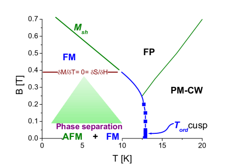
In this compound, the only phase transition observed is that between the paramagnetic PM and the ordered phase at , which vanishes around T, see Fig. 8. At higher fields it can be traced as a shoulder in (see Fig. 4a) labeled , where the linear increase turns towards saturation. The green triangle in Fig. 8 indicates how the intensity of the AFM component decreases with increasing field, from about 60% (at ) of the ordered phase to zero at . At this field, the thermodynamic relation: is confirmed between K in the magnetic and thermal properties. Above this field, the ground state mostly behaves as FM, and above one sees the crossover from the Curie-Weiss law (PM-CW) to a field polarized (FP) region.
V Conclusions
We have seen that the FM and AFM contributions can be quantitatively separated from the magnetic susceptibility signal by taking the temperature dependence of the neutron counts collected for the FM component as a reference. Though this result does not provide information on the spatial distribution of these phases, the simple additive character of both signals suggests that it is not an ’in situ’ coexistence, rather an independent distribution in the volume of two different order parameters. As it can be deduced from the magnetic susceptibility and the magnetization behavior under magnetic field, the FM phase rapidly overcomes the AFM phase
The anomalous evolution of the magnetization with temperature between 2 and 10 K shown in Fig. 4a, together with that of the entropy: for T, see Fig. 6a, indicate the increasing presence of the AFM phase at low temperatures and low fields. This peculiar situation provides the conditions for an experimental verification of the thermodynamic ralation , which is confirmed by the temperature independent susceptibility at T included in the inset of Fig. 4a.
Another unexpected feature of this compound is the non-mean field behavior of , Fig. 5. This dependence does not correspond to a Zeeman energy distribution of the eight fold ground state of the Eu2+ atoms, which are split by the internal molecular field. Notably, at zero field the data are better described by the case than by the . However at T, which is stronger than the molecular field, the better approach is the one with two sets of quartets.
Strictly speaking, this scenario is not only observed in this Eu2+ compound, but also in GdCoIn5, which is included in Fig. 5 for comparison. In all cases, the character of the orbital number inhibits pointing to a particular electronic configuration for this anomalous behavior. However, since magnetic anisotropy characterizes these compounds, the non-isotropic magnetic environment may be responsible for the observed distortion. Thus, the anisotropic distribution of magnetic interactions with neighboring magnetic atoms may explain the failure of an isotropic hypothesis such as the MFA theory. Note that the degeneracy of the ground state recovered as soon as the system approaches the intrinsically isotropic paramagnetic state at , in a temperature range where the anisotropic internal field strongly decreases. A better knowledge of the role of the magnetic interactions in an anisotropic environment requires a sophisticated mathematical analysis, which eis beyond the scope of this work.
References
- [1] N. Kumar, S.K. Dar, A. Thamizhavel, in: Magnetic properties of EuPtSi3 single crytals, Phys. Rev. B 81 (2010) 144414.
- [2] S.Seiro, C. Geibel, in: Complex and strongly anisotropic magnetism in the pure spin system EuRh2Si2, J. Phys. Condens. mtter 26 (2014) 046002.
- [3] I. Čurlík, M. Giovannini, F. Gastaldo, A. M. Strydom, M. Reiffers, J. G. Sereni, in: Crystal structure and physical properties of the two stannides EuPdSn2 and YbPdSn2; J. Physics: Cond. Mat. 30 (2018) 495802.
- [4] M. Giovannini, I. Čurlík, R. Freccero, P. Solokha, R. Reiffers, J. Sereni, in: Crystal Structure and Mgnetism of Noncentrosymmetric Eu2PdSn2, Inoganic Chemistry 60 (2021) 8085.
- [5] Z. Zhao, R. Zhang, H. Somg, Y. Zhang, X. Wu, D. Li, B. Li; in: Site selective and enhanced blue emitting of Eu2+ activated fluorapatite-type phosphors with high color purity for NUV excited pc-wLEDs; Optical Materials Express 12 (2022) 4117.
- [6] T.G. Naghiyev, U.R. Rzayev, E.M. Huseynov, I.T. Huseynov, S.H. Jabarov; in: Effect of the europium doping on the calcium sulphide: structural and thermal aspects; UNEC Journal of Engineering and Applied Sciences 2 (2022) 85-91.
- [7] R.B. Homer and B.D. Mortimer; in: Europium II as a replacement for Calcium II in Concanavalin A; FEBS Lett.87 (1978) 69.
- [8] A.L. Batchev, Md.M. Rashid, M.J. Allen; in: Divalent europium-based contrast agents for magnetic resonance imaging; Handbook on the Physics and Chemistry of Rare Earths, Eds. J-C. G. Bunzli, S.M. Kauzlarich, Ch. 328, Vol. 63 (2023) Pgs. 55-98
- [9] A. Martinelli, D. Ryan, J.G. Sereni, C. Ritter, A. Leineweber, I. Čurlik, R. Freccero, M. Giovannini; in Magnetic phase separation in EuPdSn2 ground state; J. Mater. Chem. C 11 (2023) 7641.
- [10] A. I. Akhiezer, V. G. Bar’jachtar, S V Peletminskii; in: Spin Waves, North-Holland series in Low Temperature Physics, Vol 1 , 1968.
- [11] P.H.E. Meijer, J.H. Colwell, B.P. Shah, in: A note on the Morphology of Heat Capacity curves, Am. Jour. Phys. 41 (1973) 332.
- [12] A. Szewczyk, R.J. Radwański, J.J.M. Franse, H. Nakotte; in: Heat capacity of GdNi5; JMMM 104 (1992) 1319.
- [13] D. Betancourth, J.I. Facio, P. Pedrazzini, C.B.R. Jesus, P.G. Pagliuso, V. Vildosola, P.S. Cornaglia, D.J. García, V.F. Correa; in: Low-temperature magnetic properties of GdCoIn5, JMMM 374 (2015) 744.
- [14] D. Vollhardt, in: Characteristic Crossing Points in Specific Heat Curves of Correlated Systems, Phys. Rev. Lett. 78, 1307 (1997).