Contact surgery numbers of and
Abstract.
We classify all contact structures with contact surgery number one on the Brieskorn sphere with both orientations. We conclude that there exist infinitely many non-isotopic contact structures on each of the above manifolds which cannot be obtained by a single rational contact surgery from the standard tight contact 3-sphere. We further prove similar results for some lens spaces: We classify all contact structures with contact surgery number one on lens spaces of the form . Along the way, we present an algorithm and a formula for computing the Euler class of a contact structure from a general rational contact surgery description and classify which rational surgeries along Legendrian unknots are tight and which ones are overtwisted.
Key words and phrases:
Contact surgery numbers, Legendrian knots, -invariant, Euler class2020 Mathematics Subject Classification:
53D35; 53D10, 57K10, 57R65, 57K10, 57K331. Introduction
A fundamental result in -dimensional contact topology due to Ding–Geiges says that any connected orientable compact contact -manifold with co-orientable contact structure can be obtained by contact surgery on a Legendrian link in the standard tight contact -sphere [DG04]. Moreover, one can assume all contact surgery coefficients to be . Thus a natural complexity notion for a given contact -manifold is the minimal number of components required for the surgery link.
The contact surgery number of a given contact -manifold is defined to be the minimal number of components of a Legendrian link in needed to describe as a rational contact surgery along (with non-vanishing contact surgery coefficients). Similarly, we define other versions of contact surgery numbers, i.e. , , and by requiring in addition that all contact surgery coefficients of are integers, reciprocal integers, or , respectively.
In [EKO22] the study of contact surgery numbers was initiated. In particular, explicit calculations on some simple manifolds were performed and general upper bounds on contact surgery numbers were obtained. For example it was shown that the contact surgery number of a contact manifold is at most larger than the topological surgery number of the underlying smooth manifold . On the other hand, it remained unclear if this bound is sharp. And especially for tight contact manifolds certain properties of contact surgery numbers remained unclear.
In this paper, we will add new computations of contact surgery numbers on certain Brieskorn spheres and lens spaces. In particular, these results will add some previously unknown phenomena about the behavior of contact surgery numbers of tight contact structures.
1.1. The Brieskorn sphere
Let be the Brieskorn sphere with Brieskorn invariants , i.e. the Seifert fibered space presented as the surgery diagram in Figure 4. Up to contactomorphism there exists a unique Stein fillable (hence tight) contact structure on which we denote by [GS03, Theorem 4.4]. Since is a homology sphere every overtwisted contact structure is determined by its -invariant, which can take all integer values. Our first result completely classifies all contact structures on this manifold with contact surgery number .
Theorem 1.1
-
(1)
A contact structure on the Brieskorn sphere has integer contact surgery number if and only if its -invariant is of the form
-
(2)
A contact structure on the Brieskorn sphere has rational contact surgery number if and only if its -invariant is of the form
In the proof of Theorem 1.1 we will also describe all possible contact surgery diagrams of these contact structures along a single Legendrian knot. From that, we will deduce the following corollary.
Corollary 1.2
Let be any overtwisted contact structure on , then
We also have similar results for the tight contact structure.
Corollary 1.3
Let be the standard tight contact structure on , then
A rational contact surgery diagram of along a -component Legendrian link is shown in Figure 5.
We remark that this is the first tight contact structure for which we can explicitly compute the rational contact surgery number and where it does not agree with the topological surgery number of the underlying smooth manifold.
1.2. The mirror of the Brieskorn sphere
Again up to contactomorphism there exists a unique Stein fillable (hence tight) contact structure on which we denote by [GS03, Theorem 4.9], cf. [GVHM16]. Again we can completely classify the contact structures with contact surgery number .
Theorem 1.4
-
(1)
A contact structure on has integer contact surgery number if and only if its -invariant is of the form
-
(2)
An overtwisted contact structure on has rational contact surgery number if and only if its -invariant is of the form
From Theorem 1.4 we will deduce that some contact structures have unique contact surgery diagrams along Legendrian knots.
Corollary 1.5
If is a Legendrian knot in such that contact -surgery or contact -surgery along yields a contact structure on . Then is isotopic to the unique Legendrian realization of the twist knot with and , the contact surgery coefficient is , and is isotopic to the overtwisted contact structure with . This contact surgery diagram is shown in Figure 6.
If we allow reciprocal integer contact surgery coefficients, then this contact structure has exactly one more surgery diagram: contact -surgery along the Legendrian realization of the right-handed trefoil with and , shown in Figure 6.
For the tight contact structure, we can compute all contact surgery numbers.
Corollary 1.6
If is a Legendrian knot in such that for some , contact -surgery is contactomorphic to , then is isotopic to the right-handed trefoil with and and .
In particular, we compute its contact surgery numbers as
We remark that this is the first tight contact structure for which we have explicitly computed all different versions of the contact surgery numbers and where and differ.
1.3. Integral surgery numbers of lens spaces
For , we denote by the lens space obtained by topological -surgery on the unknot . We call this surgery diagram the standard surgery diagram of . If we denote by the meridian of this unknot we know that is isomorphic to generated by . The Euler class of a -plane field on is Poincaré dual to a first homology class which we always present in this identification with . In other words if we write that a contact structure on a lens space of the form has Euler number for an integer , then we consider modulo and see it as an element in which we identify with under the above identification, i.e. we identify with the element .
The tight contact structures on are classified by Honda [Hon00]. In particular, any tight contact structure can be obtained by rational contact surgery on a Legendrian unknot (and thus has ), two tight contact structures on a lens space are distinguished by their Euler classes.
For the tight contact structures, we can compute all contact surgery numbers. In particular, there are exactly non-contactomorphic tight contact structures on that have integer contact surgery number one.
Theorem 1.7
Let be the tight contact structure on the lens space with Euler class . Then their contact surgery numbers are as follows:
| otherwise. |
We conclude that several tight contact structures on these lens spaces have unique contact surgery diagrams along a single Legendrian knot.
Corollary 1.8
Let and let be a Legendrian knot in such that for contact -surgery along yields . Then is the unique Legendrian realization of with and and the contact surgery coefficient is .
For the overtwisted contact structures we can completely classify the contact structures with and with . In general it follows from [EKO22] that any overtwisted contact structure on has . Since the first homology has no -torsion overtwisted contact structures are completely determined by their Euler class and their -invariants [Gom98, DGS04].
Theorem 1.9
-
(1)
An overtwisted contact structure on has contact surgery number if and only if its tuple of Euler class and -invariant is of the form
-
(2)
An overtwisted contact structure on has contact surgery number if and only if it appears in the list of or if its tuple of Euler class and -invariant is of the form
In particular, the above result implies the following.
Corollary 1.10
-
(1)
For any given there exists exactly one overtwisted contact structure on with Euler class that has .
-
(2)
For a given there exists infinitely many pairwise non-contactomorphic contact structures on with Euler classes that have . And there exist also infinitely many pairwise non-contactomorphic contact structures on with Euler classes that have .
1.4. Rational surgery numbers of lens spaces
We also have similar results for rational contact surgery numbers. All tight contact structures on lens spaces have . We also classify the overtwisted contact structures on that have in Theorem 4.2. But here the result is much more evolved, so in this introduction, we only state one of its corollaries.
Corollary 1.11
For every given there exists infinitely many pairwise non-contactomorphic contact structures on that have .
1.5. Outline of the arguments
We briefly outline our main arguments. Let be either the Brieskorn sphere or a lens space which is of the form . Then there are results of Culler–Gordon–Luecke–Shalen [CGLS87], Baldwin–Sivek [BS22], and Rasmussen [Ras07] that together completely classify all surgery diagrams along a single knot yielding . It turns out that these are all surgeries along unknots, certain torus knots, and twist knots for which the classification of Legendrian realizations is known [EF98, EH01, ENV13, CN]. Moreover, the classification of tight contact structures on is known by [Hon00, GS03] and the overtwisted contact structures are determined by their homotopical invariants [Eli89]. Since is a rational homology sphere that has no -torsion in its first homology, these homotopical invariants are given by the Euler class, and the -invariant [Gom98, DGS04]. Thus we can enumerate all possible contact surgery diagrams along a single Legendrian knot in yielding a contact structure on . Then we check which of these surgeries yield tight and which yield overtwisted manifolds. We use the formulas from [DK16] to compute their homotopical invariants. This yields the classification of contact structures on that have contact surgery number from which we can deduce the claimed results. Opposed to the results obtained in [EKO22], here we also need to work with Legendrian non-simple knots (the Legendrian twist knots) and since we do not just work on homology spheres, we have more complicated surgery coefficients and need to take the Euler classes into account. For that we discuss in Theorem 2.3 how to compute the Euler classes of general rational contact surgery diagrams which might be of independent interest. In Section 2 we recall the needed background on contact surgery and in Section 4 we present the details of the above arguments.
Conventions
All contact structures are assumed to be positive and coorientable. We present Legendrian knots always in their front projection. Since a contact surgery diagram determines a contact manifold only up to contactomorphism, we consider contact manifolds only up to contactomorphism (and not up to isotopy). Moreover, the contactomorphism type of a contact surgery is independent of an orientation of the Legendrian surgery link. Thus we mainly consider unoriented Legendrian links in up to isotopy of unoriented links. Then the rotation number of an unoriented Legendrian knot is only defined up to sign. For some calculations, it will be helpful to choose orientations on Legendrian links in which case the rotation numbers are always understood with signs. We normalize the invariant such that as done for example in [CEK21, EKO22, KO23]. With that normalization, the -invariant is additive under connected sum and takes integer values on homology spheres.
Acknowledgments
The authors are supported by SFB/TRR 191 Symplectic Structures in Geometry, Algebra and Dynamics, funded by the Deutsche Forschungsgemeinschaff (Project-ID 281071066-TRR 191).
We would like to thank John Etnyre for many helpful suggestions and discussions.
This work started in February 2023 at the conference Winterbraids XII in Tours and was continued at the workshop and summer school on Low-Dimensional Topology at IISER Pune. We thank the organizers of both events for their support. The authors wish to thank Peter Albers, for his hospitality when R.C. visited the University of Heidelberg. Part of the writing was done when R.C. was visiting the Max-Plank Institute of Mathematics in Bonn. She expresses her gratitude for their hospitality.
2. Preliminaries
In this section, we briefly recall the necessary background on contact surgery and how to compute the homotopical invariants of a contact structure from one of its contact surgery diagrams. For background on contact geometry, we refer to [Gei08]. For more on contact surgery and the homotopical invariants of contact structures, we refer to [Gom98, DG04, DGS04, OS04, DK16, Keg17, Keg18, CEK21, EKO22].
2.1. Contact surgery
Let be a Legendrian knot in . We perform Dehn surgery on with contact surgery coefficient (i.e. measured with respect to the contact longitude of , obtained by pushing into the Reeb-direction). Then there exist (up to contactomorphism) finitely many tight contact structures on the newly glued-in solid torus that fit together with the old contact structure to give a global contact structure on the surgered manifold [Hon00]. We write for one of these contact manifolds obtained by contact -surgery along . If in addition, the contact surgery coefficient is of the form , for , then the contact structure on the surgered manifold is unique up to contactomorphism.
It will be convenient to introduce the following notation. We write for the Legendrian link consisting of together with a Legendrian push-off of . We denote a copy of with extra stabilizations by . Here the -extra stabilizations are not specified but fixed. If the knot is again stabilized times this is denoted by .
Lemma 2.1 (Ding–Geiges [DG01, DG04])
Let be a Legendrian knot in .
-
(1)
Cancellation lemma: For every , we have
-
(2)
Replacement lemma: For every , we have
-
(3)
Transformation lemma: For every and every integer , we have
If the contact surgery coefficient is negative, one can write uniquely as
with integers and we have
In addition, all these results hold true in a tubular neighborhood of . In particular, they can be applied to knots in larger contact surgery diagrams.
2.2. The homotopical invariants
We will also need to compute the algebraic invariants of the underlying tangential -plane field of a contact structure. It is known that a tangential -plane field on a rational homology sphere with no -torsion in , is completely determined by its Euler class and its -invariant [Gom98, DGS04]. Roughly speaking, the Euler class determines on the -skeleton of , while the -invariant gives on the -cell of . For contact -surgeries these invariants can be computed with the following result from [DK16].
Lemma 2.2
Let be a Legendrian link in and denote by the contact manifold obtained from by contact -surgeries along , with . After choosing an orientation on we write , for the Thurston–Bennequin invariant and the rotation number of , and for the linking number of and . We denote the topological surgery coefficient of by and define the generalized linking matrix as
-
(1)
Then is a presentation matrix for the first homology group of , i.e. is generated by the meridians and the relations are where is the vector with entries .
-
(2)
If all , the Euler class is Poincaré dual to
-
(3)
The Euler class is torsion if and only if there exists a rational solution of , where is the vector of the rotation numbers . In this case, the -invariant is a well-defined rational number and computes as
where denotes the sign of the contact surgery coefficient of and denotes the signature of . (In the proof of Theorem 5.1. in [DK16] it is shown that the eigenvalues of are all real and thus the signature of is well-defined although is in general a non-symmetric matrix.)
Next, we present a formula and an algorithm how to compute the Euler class of a contact structure from a general rational contact surgery diagram. Here the main idea is to use the transformation lemma to transform a general contact surgery diagram into one with only -contact surgery coefficients. We will perform that process by doing explicit Kirby moves which will allow us to keep track of the meridians. Then we can use Lemma 2.2 to compute the Euler class.
Theorem 2.3
Let be a contact manifold that is obtained by rational contact surgery on an oriented Legendrian link in . Let be a component of with contact surgery coefficient . Then the Euler class of can be represented in the basis of given by the meridians of by
where is an integer, is the meridian of , and is a linear combination of the meridians of .
On the other hand, the transformation lemma tells us that there exist integers such that
| (1) |
We denote the components of the above surgery description as for and write and for the Thurston–Bennequin invariant and rotation number of , and for the rotation number and for the meridian of .
We have the following cases:
-
(1)
For , the surgery diagram reduces to In the basis of given by this surgery description the Euler class is given by
-
(2)
For , i.e for contact -surgery and for and for , i.e for contact surgery the Euler classes are given by
-
(3)
For and , in the basis of given by the surgery description from Equation 1 the Euler class is given by
This case corresponds to negative contact surgery.
-
(4)
For , and , in the basis of given by the surgery description from Equation 1 the Euler class is given by
The main ingredients in the proof of the above theorem are the following two lemmas.
Lemma 2.4
Under the diffeomorphism from Equation 1, for and the homology classes of the meridians in are mapped as follows:
For , the meridians are mapped as follows:
For , we have the following:
Proof.
We will consider several cases of increasing difficulty.
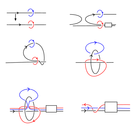
Case 1: First we consider the case that for a positive integer . This is equivalent of saying that . We will show by induction on that
The induction step follows from the Kirby moves in Figure 1. We start in with the Kirby diagram
and their meridians and end up with their images in
under the Kirby moves in diagram from which we read-off that
where we write for the -th knot in the surgery diagram . The statement then follows from the induction hypothesis.
2pt \pinlabel at 180 720 \pinlabel at 180 645 \pinlabel at 250 700 \pinlabel at 250 630 \pinlabel at 180 570 \pinlabel at 580 720 \pinlabel at 650 637 \pinlabel at 690 700 \pinlabel at 710 600 \pinlabel at 620 570 \pinlabel at 180 540 \pinlabel at 180 440 \pinlabel at 280 440 \pinlabel at 310 380 \pinlabel at 180 300 \pinlabel at 620 300 \pinlabel at 580 530 \pinlabel at 650 340 \pinlabel at 710 380 \pinlabel at 610 430 \pinlabel at 180 20 \pinlabel at 302 120 \pinlabel at 200 250 \pinlabel at 270 70 \pinlabel at 620 20 \pinlabel at 650 120 \pinlabel at 730 160 \pinlabel at 560 140 \pinlabel1+ at 633 605
Case 2: Next, we consider a surgery diagram where has contact surgery coefficient and all other ’s have contact surgery coefficient . We will show by induction that
The induction step (for ) follows also along the same lines as Case from the Kirby moves depicted in Figure 2. From Figure 2 we read-off that
where we write for the -th knot in the surgery diagram . The statement then follows from the induction hypothesis.
2pt
\pinlabel at 150 710
\pinlabel at 150 640
\pinlabel at 275 700
\pinlabel at 255 630
\pinlabel at 150 560
\pinlabel at 620 720
\pinlabel at 660 650
\pinlabel at 700 700
\pinlabel at 600 560
\pinlabel at 135 510
\pinlabel at 170 440
\pinlabel at 160 310
\pinlabel at 300 450
\pinlabel at 600 300
\pinlabel at 520 490
\pinlabel at 460 330
\pinlabel at 620 420
\pinlabel at 160 10
\pinlabel at 110 220
\pinlabel at 115 80
\pinlabel at 270 190
\pinlabel at 325 150
\pinlabel at 600 10
\pinlabel at 530 160
\pinlabel at 654 150
\pinlabel at 510 90
\pinlabel- at 49 647
\pinlabel- at 410 647
\pinlabel at 657 610
\endlabellist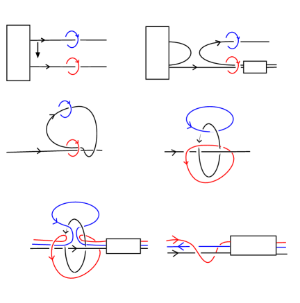
Case 3: The general case is smoothly depicted in Figure 3. First, we just look at the last components starting from . Notice that this coincides with Case . And thus we get
2pt
\pinlabel at 155 220
\pinlabel at 100 210
\pinlabel at 55 150
\pinlabel at 362 275
\pinlabel at 300 267
\pinlabel at 492 250
\pinlabel at 130 100
\pinlabel at 210 100
\pinlabel at 470 30
\pinlabel at 470 70
\pinlabel at 305 100
\pinlabel at 470 100
\pinlabel at 470 130
\pinlabel at 470 150
\pinlabel at 330 180
\pinlabel at 330 220
\pinlabel at 400 220
\pinlabel at 400 180
\pinlabel at 485 270
\endlabellist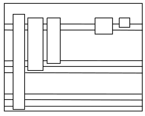
Here again denotes the meridian of after the Kirby moves. Now we can forget about the components with index larger than and just look at the components . This part coincides with Case . Thus we have
Together this implies the general case of the lemma.
For , the proof works the same. One just needs to keep track of the meridian as in Figure 1. The only difference will be that will have topological surgery coefficient . ∎
Lemma 2.5
For negative contact surgery, under the diffeomorphism from Equation 1 with , the homology classes of the meridians for in are mapped as follows:
For , the meridians are mapped as follows:
For contact -surgery, we have the following:
Proof.
The proof is similar to the proof of Lemma 2.4. ∎
3. Tight surgeries on Legendrian unknots
In this section, we will classify which rational contact surgeries on Legendrian unknots yield tight contact manifolds and which yield overtwisted contact manifolds. Our main result reads as follows.
Theorem 3.1
Let be a Legendrian unknot with . Then is tight if and only if
-
(1)
, or
-
(2)
and is only stabilized with one sign (or not stabilized at all) and the first stabilization of in the transformation lemma has the same sign as the stabilizations of (or has arbitrary sign in case that is not stabilized).
We first start with a simple lemma.
Lemma 3.2
Let be a Legendrian unknot with . Then every is overtwisted if .
Proof.
Let for coprime integers . We denote by a Legendrian meridian of with seen as a knot in . Then can also be seen as a rational Legendrian unknot in , and thus any rational Seifert surface of in has Euler characteristic . On the other hand, we compute, for example with [Keg17, Section 4.5], the rational Thurston–Bennequin invariant of in to be . Thus violates the rational Bennequin inequality [BE12] in which implies that is overtwisted. ∎
Proof of Theorem 3.1.
First, we recall that contact surgery with a negative contact surgery coefficient preserves fillability. In particular, is tight whenever . Thus in the following, we will restrict to positive contact surgery coefficients.
We denote by the Legendrian unknot with Thurston–Bennequin invariant . Then it follows from Lemma 3.2 that is overtwisted for . If , we can use the transformation lemma to write
Since yields the tight contact structure on and is negative, it follows that every is tight. Together with Lemma 3.2 we have shown that is overtwisted if and only if .
Now we denote by a Legendrian unknot with Thurston–Bennequin invariant . If is stabilized with two different signs then every , , is overtwisted [Ozb06], cf. [EKO22, Theorem 3.3]. So we assume from now that is stabilized with only one sign, i.e. . If then is always overtwisted by Lemma 3.2. Next, we consider the case . We choose coprime integers , such that . Then and
Thus the first terms in the negative continued fraction expansion read as
Then the transformation lemma yields
If the extra stabilization of has a different sign than the stabilizations of then the contact structure is overtwisted [EKO22, Theorem 3.3] if the extra stabilization has the same sign we use the lantern destabilization [LS11, EKO22] and the transformation lemma again to write
Inductively, this implies
and since it follows that this contact structure is tight as claimed. ∎
4. Proofs of the main results
4.1. The Brieskorn sphere
Proof of Theorem 1.1.
Let be contactomorphic to for some Legendrian knot in and some . Then a recent result of Baldwin–Sivek [BS22] says that either is a Legendrian realization of the positive twist knot with topological surgery coefficient or is a Legendrian realization of the left-handed trefoil knot with topological surgery coefficient . These surgery diagrams are shown in Figure 4.
To prove statement , we only need to consider the first possibility (since the latter will always yield a rational contact surgery). Since is Legendrian simple, every Legendrian realization of is obtained by stabilizing the unique Legendrian representative of with and [ENV13]. Then we can readily apply Corollary 4.7 from [EKO22] to deduce statement .
For , we also need to consider Legendrian realizations of the left-handed trefoil. Let be a Legendrian left-handed trefoil. From the classification of Legendrian realizations of , we deduce that has Thurston–Bennequin invariant [EH01]. Thus yields a contact structure on . (And together with the contact structures obtained in this is the complete list of contact structures on with .) We compute the possible -invariants of these contact structures. For that, we use Lemma 2.1 to change the contact surgery diagram into one with only reciprocal integer coefficients, so that Lemma 2.2 applies. We apply the transformation lemma to see that
where the last equality comes from the negative continued fraction expansion
| (2) |
From this surgery description, we deduce the generalized linking matrix to be
Next, we compute the signature of to be and solve from which we get the -invariants. We write for the rotation number of . In the case of , we get
and for , we compute
By writing for the claimed formulas follow. ∎
Proof of Corollary 1.2.
In the proof of Theorem 1.1 we created all contact surgery diagrams along a single Legendrian knot yielding contact structures on . The lower bound of the corollary follows by observing that these were all with contact surgery coefficients not of the form of a reciprocal integer. The upper bound follows from Proposition 6.8 in [EKO22]. ∎
Proof of Corollary 1.3.
Figure 5 shows how to obtain a contact surgery diagram of along a two-component Legendrian link. This yields the upper bound of for and by applying the transformation lemma it also yields the upper bound for . For the lower bound, we compute and observe that is never attained for the possible -invariants in Theorem 1.1. Finally, the upper bound of for is given by Theorem 6.9 in [EKO22]. ∎
4.2. The mirror of the Brieskorn sphere
Proof of Theorem 1.4.
First, we observe that if topological -surgery (i.e. with respect to the Seifert framing) along a smooth knot yields the smooth manifold , then -surgery along the mirror of yields the mirrored manifold . Thus we can deduce from [BS22] that any Legendrian knot such that yields a contact structure on is either isotopic to a Legendrian realization of with topological surgery coefficient or isotopic to a Legendrian realization of the right-handed trefoil with topological surgery coefficient . Since the classification of all Legendrian realizations of [EH01] and [ENV13] are known, the same strategy as above works.
Statement follows directly from the classification of Legendrian realization of and Corollary 4.76 from [EKO22].
For statement we consider a Legendrian realization of the right-handed trefoil with Thurston–Bennequin invariant . Then yields a contact structure on . For this corresponds to a contact -surgery. Since negative surgery preserves tightness [Wan15] the resulting contact structure is contactomorphic to the standard tight contact structure , with . If , we perform a contact -surgery and we compute directly that . For , we use Lemma 2.1 to change the contact surgery diagram to
where the last equality comes from the negative continued fraction expansion from Equation (2). From that, we deduce the generalized linking matrix to be
Next, we compute the signature of to be and solve from which we get the -invariants. We write for the rotation number of . In the case of , we get
and for , we compute
By writing for the claimed formulas follow. ∎
Proof of Corollary 1.5.
Proof of Corollary 1.6.
4.3. Surgery diagrams of the lens spaces
Recall from the introduction that for an integer we can represent in its standard surgery diagram: The -surgery along the unknot .
As preparation for the classification of the contact structures on that have contact surgery number we enumerate in this section all smooth surgery diagrams of along a single knot . Moreover, we will present the meridians of these surgery knots in the standard basis of generated by the meridian of the unknot in the standard surgery description. The result is as follows.
Theorem 4.1
Let be a knot in and be a surgery coefficient measured with respect to the Seifert framing such that is diffeomorphic to . Then is either
-
•
the torus knot with surgery coefficient , or
-
•
an unknot with surgery coefficient for an integer , or
-
•
an unknot with surgery coefficient for an integer .
Moreover, the meridians , , and of the torus knot , , and can be expressed in the standard basis as
Proof.
First, the cyclic surgery theorem [CGLS87] implies that is either an unknot or is an integer. If is an integer then a result of Rasmussen [Ras07] implies that is isotopic to the torus knot with surgery coefficient .
If is an unknot then the classification of lens spaces gives us all surgery diagrams along unknots yielding . For that, we consider the surgery plumbing graph corresponding to the continued fraction expansion of this lens space. I.e. we consider the positive Hopf link with surgery coefficients on the first component and surgery coefficient on the second component shown in Figure 7.
2pt
\pinlabel at 370 250
\pinlabel at 160 250
\pinlabel at 35 150
\pinlabel at 370 150
\endlabellist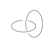
By slam dunking away, we get the standard surgery diagram of . In Figure 8 we keep track of the meridians and of and under this slam dunk, which shows that under the slam dunk diffeomorphism, the meridians get mapped as follows
2pt
\pinlabel at 150 750
\pinlabel at 60 650
\pinlabel at 75 550
\pinlabel at 400 650
\pinlabel at 220 600
\pinlabel at 370 750
\pinlabel at 250 440
\pinlabel at 630 750
\pinlabel at 840 750
\pinlabel at 900 650
\pinlabel at 610 520
\pinlabel at 740 410
\pinlabel at 300 400
\pinlabel at 420 360
\pinlabel at 460 300
\pinlabel at 140 210
\pinlabel at 450 120
\pinlabel at 290 220
\pinlabel at 270 50
\pinlabel at 110 290
\pinlabel at 760 40
\pinlabel at 610 210
\pinlabel at 930 290
\pinlabel at 600 290
\pinlabel at 780 220
\pinlabel at 910 95
\pinlabel--1 at 661 572
\endlabellist
For any integer we can perform a Rolfsen twist on the standard surgery description to get again an unknot but with the surgery coefficient changed to . The Rolfsen twist does not change the homology class of the meridian and thus
Finally, there are the dual surgery descriptions (which we get by interchanging the roles of the two Heegaard tori in the above surgery descriptions). In the surgery picture we obtain these by slam dunking away in Figure 7. This yields an unknot with surgery coefficient . This dual slam dunk diffeomorphism sends to and thus
By performing a -fold Rolfsen twist on we get the surgery descriptions on with surgery coefficient . The Rolfsen twist does not change the homology class of the meridian of and thus
The classification of lens spaces implies that this is the complete list of -component surgery descriptions of .
It remains to express as a multiple of . For that, we refer to Figure 9 in which a sequence of Kirby moves from the surgery diagram along the torus knot to the dual surgery description is presented. In that figure, we observe that gets mapped to and thus we obtain
as claimed. ∎
2pt
\pinlabel at 60 650
\pinlabel at 130 570
\pinlabel at 130 530
\pinlabel at 5 530
\pinlabel at 337 520
\pinlabel at 300 650
\pinlabel at 170 360
\pinlabel at 670 520
\pinlabel at 530 470
\pinlabel at 640 650
\pinlabel at 430 650
\pinlabel at 530 360
\pinlabel at 900 360
\pinlabel at 900 560
\pinlabel at 1000 650
\pinlabel at 750 470
\pinlabel at 759 570
\pinlabel at 400 10
\pinlabel at 220 300
\pinlabel at 370 200
\pinlabel at 800 10
\pinlabel at 800 300
\pinlabel at 920 120
\endlabellist
4.4. Integral contact surgery numbers of the lens spaces
Proof of Theorem 1.7.
By Honda’s classification of tight contact structures on lens spaces [Hon00] any tight contact structure can be obtained by Legendrian surgery on a chain of Legendrian unknots. For a lens space of the form the complete list of tight contact structures is given by the surgery descriptions shown in Figure 10. In particular, it follows that any tight contact structure on such a lens space has contact surgery number .
2pt
\pinlabel at 230 80
\pinlabel at 465 80
\pinlabel at 230 360
\pinlabel at 430 360
\pinlabel at 650 150
\pinlabel at 50 150
\endlabellist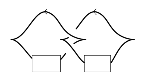
Now let be a tight contact structure on that is contactomorphic to for some Legendrian knot in and some . Then Theorem 4.1 implies that is a Legendrian realization of the torus knot with topological surgery coefficient . By [EH01], torus knots are Legendrian simple and the torus knots at hand have . There are exactly different Legendrian realizations of with Thurston–Bennequin invariant . These have rotation numbers and are shown in Figure 11. Legendrian surgery on any of these Legendrian realizations yields a tight contact structure on . From Lemma 2.2 we see that the Poincaré dual of the Euler class is given by . Using Theorem 4.1 we can express the Euler class in the standard basis to see that the tight contact structures claimed in Theorem 1.7 all have contact surgery numbers .
To see that the other tight contact structures have , we observe that any other integer surgery on a Legendrian realization of that yields a contact structure on is along a stabilized knot with a positive surgery coefficient and thus is overtwisted by [LS11].
The same argument yields the result for the integer contact surgery numbers. ∎
Proof of Corollary 1.8.
Next, we study the overtwisted contact structures on .
Proof of Theorem 1.9.
Let be a contact structure on that is contactomorphic to for some Legendrian knot in and some . The same argument as in the proof of Theorem 1.7 shows that is a Legendrian realization of with Thurston–Bennequin invariant and the topological surgery coefficient is .
If the contact structure is tight and was already handled in the proof of Theorem 1.7. We do not need to consider the case when since then the contact surgery coefficient would vanish.
We recall that any other integer surgery on a Legendrian realization of that yields a contact structure on is along a stabilized knot with a positive surgery coefficient and thus is overtwisted by [LS11].
If , the contact surgery coefficient is . Thus the generalized linking matrix is and we can readily apply Lemma 2.2 to compute that and
where denotes the rotation number of . From [EH01] we see that the possible range of rotation numbers of Legendrian realizations of with is given by , for . Plugging this in yields the formulas claimed in .
Next, we assume that . Then the contact surgery coefficient is . Thus we deduce from the transformation lemma 2.1 that
| (3) |
From this surgery description, we compute the generalized linking matrix to be
We first compute the -invariants. For that we observe the signature of to be and solve (where denotes again the rotation number of ) from which we get
From [EH01] we conclude that , for , which directly yields the claimed formula for the -invariants in .
4.5. Rational contact surgery numbers of the lens spaces )
For the rational contact surgery numbers the same strategy works to classify all contact structures on that have . However, here we have to consider several infinite families of contact surgery diagrams given by Legendrian realizations of the smooth surgery diagrams given in Theorem 4.1. The main result is as follows.
Theorem 4.2
| (3) | |
|---|---|
| for | |
| (4) | |
| for | |
| (5) | |
| for | |
| (6) | |
| for | |
| (7) | |
| for | |
| (8) | |
| for | |
| (9) | |
| for | |
| (10) | |
| for | |
| (11) | |
| for | |
| (12) | |
| for | |
| (13) | |
| for | |
| (14) | |
| for | |
| (15) | |
| for | |
| (16) | |
| for | |
| (17) | |
| for | |
| (18) | |
| for | |
| (19) | |
| for | |
| (20) | |
| for |
| (21) | |
|---|---|
| for | |
| (22) | |
| for | |
| (23) | |
| for | |
| (24) | |
| for | |
| (25) | |
| for | |
| (26) | |
| for | |
| (27) | |
| for | |
| (28) | |
| for | |
| (29) | |
| for | |
| (30) | |
| for |
Proof.
Let be a Legendrian knot such that contact -surgery, , on yields an overtwisted contact structure on . The case that is an integer was already discussed in Theorem 1.9. Thus here we concentrate on the case that . From Theorem 4.1, we know that is a Legendrian realization of the unknot and that the topological surgery coefficient is or for .
Now the strategy is the same as in the proof of Theorem 1.9. We will enumerate all possible contact surgery diagrams and compute their homotopical invariants. For that we convert the topological surgery coefficient into a contact surgery coefficient. We denote by the Thurston–Bennequin invariant of . Then it follows that
Next, we consider the different possibilities for , , possible rotation numbers of , and the possible stabilizations in the transformation lemma. In all of these cases we first use Theorem 3.1 to sort out the tight contact structures (these all have by Honda’s classification [Hon00]) and for the remaining overtwisted contact structures we compute and with the methods from Section 2.
We start with the simplest case, where we choose and thus the contact surgery coefficient simplifies to . We need to consider three subcases here. In Table 1, these correspond to Families (3), (4) and (5).
Family (5): For this corresponds to a contact -surgery, which is overtwisted by Theorem 3.1. To compute we see that the generalized linking matrix is with signature . This yields
with the rotation number for . The Euler class is simply given by .
Family (3): For we see that and thus it yields overtwisted manifolds by Theorem 3.1. Applying the transformation lemma, we get
The generalized linking matrix for this case is given by
To get the invariants, we compute the signature of to be and solve where . Note that, we are only considering the classification up to contactomorphism it suffices for us to consider only. Now a straightforward calculation yields
Family (4): Note that when , we have a slightly different surgery diagram as in Family (3) and thus we have to compute the -invariant separately. Here the resulting contact structures are again overtwisted by Theorem 3.1. In this case, the generalized linking matrix is
with signature We solve where is the rotation number of the first component and . Solving this gives us
As , we can rewrite where To calculate the Euler class, we simply plug in the corresponding values in the formula from Theorem 2.3.
Finally, for , the contact surgery coefficient is negative and thus yield tight contact structures, which we do not consider here.
For , the calculation is much more involved. So, we just present a single example case here.
Family (14): We consider the first contact surgery coefficient with . Then is positive and from Theorem 3.1 it follows that these contact structures are overtwisted if and only if . Thus we assume . Applying the transformation lemma 2.1 we get
The generalized linking matrix is
with signature . We solve
where denote the rotation number of the corresponding components. Rewriting , , and with and . By writing and plugging everything into the formulas from Lemma 2.2 and Theorem 2.3 we get the claimed values for and .
| (3) | |||
|---|---|---|---|
| (4) | |||
| (5) | |||
| (6) | |||
| (7) | |||
| (8) | |||
| (9) | |||
| (10) | |||
| (11) | |||
| (12) | |||
| (13) | |||
| (14) | |||
| (15) | |||
| (16) | |||
| (17) | |||
| (18) | |||
| (19) | |||
| (20) | |||
| (21) | |||
| (22) | |||
| (23) | |||
| (24) | |||
| (25) | |||
| (26) | |||
| (27) | |||
| (28) | |||
| (29) | |||
| (30) |
Families (6)-(13): These families correspond to the different possibilities of with that yield overtwisted contact structures.
Families (15)-(30): These families correspond to the different possibilities of that yield overtwisted contact structures.
In Table 3 we have listed the surgery diagrams of the above families. ∎
From Theorem 4.2 we can deduce Corollary 1.11 which was stated in the introduction. More precisely, we will prove the following.
Corollary 4.3
For every and every there exists a unique overtwisted contact structure on with homotopical invariants
For any odd integer we have .
Proof of Corollary 1.11.
First, we prove the existence of the contact structures . We distinguish by the parity of . If , we consider the tight contact structure on with surgery diagram from Figure 10 with . From that diagram we compute that and .
If , we consider the tight contact structure on with surgery diagram from Figure 10 with and . From that diagram we compute that and .
Now let be a contact structure on with Euler class and -invariant . For every we consider the overtwisted contact manifold
Since the -invariant behaves additive under connected sum and the Euler class does not change, we see that this contact structure has again Euler class and -invariant . This proves the existence of the overtwisted contact structures claimed in the corollary.
Since the first homology of has no -torsion, an overtwisted contact structure is uniquely determined by and and thus is uniquely determined by its homotopical invariants.
To show that infinitely many of these contact structures have we check which of the appear in the lists from Theorem 1.9 and 4.2. For that we will check which of those have homotopical invariants of the form .
(A) Obstructions from the Euler class:
Family (1): In this family the Euler class is , for . Thus the Euler class takes values between and and in particular is not or .
Family (5): The Euler class is , for . If is odd this cannot be and if is even this cannot be .
Family (4): In this family the Euler class is for and . We check that the for () the Euler class is () if and only if and . Then we plug in these values in the -invariant to see that if is even we do not get any contact structure of the desired form. On the other hand, for every odd we get a contact structure with and .
(B) Universally bounded -invariants:
Families (3), (6), (9), (20), (23), (29): In these cases we observe that is always negative.
Families (7), (8), (10)–(13), (15), (17), (22), (26), (28), (30): In these cases we can bound from above by .
Family (2): Here we observe that if the Euler class is or , then the -invariant is negative.
(C) Bounded -invariants:
Families (16), (18), (19), (21), (24), (25): In these cases we estimate to be smaller than .
(D) Even -invariants:
Families (14), (27): We will show that in these two cases it follows that if is odd (even) and () then it follows that (). In other words, the in the statement of the corollary is always an even number.
For that, we consider all possible parities of , , and and check the parities of the -invariants. We present the details for Family (14). (Family (27) works similarly.)
In Family (14) the formula for the invariant consists of -summands. The first summand is which we can ignore. The second two summands are integers and the last two summands are fractions with odd denominator .
The second term is which is odd if and only if is even. The third term is and is odd if and only if is even and is odd. The numerator of the last term is a multiple of . And the third term has even denominator if and only if is even which is the case if and only if or is odd. By adding up these parities we see that we get in all cases even values of . ∎
References
- [BE12] K. Baker and J. Etnyre, Rational linking and contact geometry, Perspectives in analysis, geometry, and topology, Progr. Math., vol. 296, Birkhäuser/Springer, New York, 2012, pp. 19–37. MR 2884030
- [BS22] J. A. Baldwin and S. Sivek, Characterizing slopes for , 2022, arXiv:2209.09805.
- [CEK21] R. Casals, J. B. Etnyre, and M. Kegel, Stein traces and characterizing slopes, 2021, arXiv:2111.00265, to appear in Math. Ann.
- [CGLS87] M. Culler, C. McA. Gordon, J. Luecke, and P. B. Shalen, Dehn surgery on knots, Ann. of Math. (2) 125 (1987), 237–300. MR 881270
- [CN] W. Chongchitmate and L. Ng, The Legendrian knot atlas, https://services.math.duke.edu/~ng/atlas/.
- [DG01] F. Ding and H. Geiges, Symplectic fillability of tight contact structures on torus bundles, Algebr. Geom. Topol. 1 (2001), 153–172. MR 1823497
- [DG04] by same author, A Legendrian surgery presentation of contact 3-manifolds, Math. Proc. Cambridge Philos. Soc. 136 (2004), 583–598. MR 2055048
- [DGS04] F. Ding, H. Geiges, and A. I. Stipsicz, Surgery diagrams for contact 3-manifolds, Turkish J. Math. 28 (2004), 41–74. MR 2056760
- [DK16] S. Durst and M. Kegel, Computing rotation and self-linking numbers in contact surgery diagrams, Acta Math. Hungar. 150 (2016), 524–540. MR 3568107
- [EF98] Y. Eliashberg and M. Fraser, Classification of topologically trivial Legendrian knots, Geometry, topology, and dynamics (Montreal, PQ, 1995), CRM Proc. Lecture Notes, vol. 15, Amer. Math. Soc., Providence, RI, 1998, pp. 17–51. MR 1619122
- [EH01] J. B. Etnyre and K. Honda, Knots and contact geometry. I. Torus knots and the figure eight knot, J. Symplectic Geom. 1 (2001), 63–120. MR 1959579
- [EKO22] J. B. Etnyre, M. Kegel, and S. Onaran, Contact surgery numbers, 2022, arXiv:2201.00157, to appear in J. Symplectic Geom.
- [Eli89] Y. Eliashberg, Classification of overtwisted contact structures on -manifolds, Invent. Math. 98 (1989), 623–637. MR 1022310
- [ENV13] J. B. Etnyre, L. Ng, and V. Vértesi, Legendrian and transverse twist knots, J. Eur. Math. Soc. (JEMS) 15 (2013), 969–995. MR 3085098
- [Gei08] H. Geiges, An introduction to contact topology, Cambridge Studies in Advanced Mathematics, vol. 109, Cambridge University Press, Cambridge, 2008. MR 2397738
- [Gom98] R. E. Gompf, Handlebody construction of Stein surfaces, Ann. of Math. (2) 148 (1998), 619–693. MR 1668563
- [GS03] P. Ghiggini and S. Schönenberger, On the classification of tight contact structures, Topology and geometry of manifolds (Athens, GA, 2001), Proc. Sympos. Pure Math., vol. 71, Amer. Math. Soc., Providence, RI, 2003, pp. 121–151. MR 2024633
- [GVHM16] P. Ghiggini and J. Van Horn-Morris, Tight contact structures on the Brieskorn spheres and contact invariants, J. Reine Angew. Math. 718 (2016), 1–24. MR 3545876
- [Hon00] K. Honda, On the classification of tight contact structures-I, Geom. Topol. 4 (2000), 309–368. MR 1786111
- [Keg17] M. Kegel, Legendrian knots in surgery diagrams and the knot complement problem, Ph.D. thesis, Universität zu Köln, 2017.
- [Keg18] M. Kegel, The Legendrian knot complement problem, J. Knot Theory Ramifications 27 (2018), 1850067, 36. MR 3896311
- [KO23] M. Kegel and S. Onaran, Contact surgery graphs, Bull. Aust. Math. Soc. 107 (2023), 146–157. MR 4531699
- [LS11] P. Lisca and A. Stipsicz, Contact surgery and transverse invariants, J. Topol. 4 (2011), 817–834. MR 2860344
- [OS04] B. Ozbagci and A. I. Stipsicz, Surgery on contact 3-manifolds and Stein surfaces, Bolyai Society Mathematical Studies, vol. 13, Springer-Verlag, Berlin; János Bolyai Mathematical Society, Budapest, 2004. MR 2114165
- [Ozb06] B. Ozbagci, An open book decomposition compatible with rational contact surgery, Proceedings of Gökova Geometry-Topology Conference 2005, Gökova Geometry/Topology Conference (GGT), Gökova, 2006, pp. 175–186. MR 2282016
- [Ras07] J. Rasmussen, Lens space surgeries and L-space homology spheres, 2007, arXiv:0710.2531.
- [Wan15] A. Wand, Tightness is preserved by Legendrian surgery, Ann. of Math. (2) 182 (2015), 723–738. MR 3418529