The Cosmological Impact of Brane-Chern-Simons Massive Gravity

Abstract

In this paper, we present a novel extension of massive gravity theory; the Brane-Chern-Simons massive gravity theory. We explore the cosmological implications of this theory by deriving the background equations and demonstrating the existence of self-accelerating solutions. Interestingly, our theory suggests the existence of self-accelerating mechanisms that originate from an effective cosmological constant, leading to intriguing possibilities for understanding the nature of cosmic acceleration. Furthermore, we perform a tensor perturbation analysis to investigate the propagation of gravitational waves in this framework. We derive the dispersion relation for gravitational waves and study their behavior in the Friedmann-Lemaître-Robertson-Walker cosmology within the context of Brane-Chern-Simons massive gravity. Utilizing the latest Union2 type Ia supernovae dataset comprising 557 SNIa events, we provide observational support for our theoretical framework, indicating that the Brane-Chern-Simons massive gravity theory is consistent with cosmological observations.

1 Introduction

The late-time accelerated expansion of the universe remains one of the most intriguing puzzles in modern cosmology, prompting extensive research into the underlying mechanisms driving this phenomenon. While the inclusion of cosmological constant or dark energy components within the framework of general relativity provides a plausible explanation Weinberg:1988cp ; Peebles:2002gy ; Copeland:2006wr ; Carroll:2003st ; Cai:2009zp ; Bamba:2012cp , alternative approaches have also gained significant attention.

Modified gravity theories offer a compelling avenue to explore, encompassing a wide range of models that modify the geometric sector of general relativity Nojiri:2010wj ; Clifton:2011jh ; CANTATA:2021ktz ; Ishak:2018his ; Abdalla:2022yfr . Within this broad category, curvature-based gravity theories, such as $f(R)$ gravity Starobinsky:1980te , $f(G)$ gravity Nojiri:2005jg , $f(P)$ gravity Erices:2019mkd , Lovelock gravity Lovelock:1971yv , and Horndeski/Galileon scalar-tensor theories Horndeski:1974wa ; Deffayet:2009wt , have been extensively studied. Another branch of modified gravity involves torsion-based theories, including $f(T)$ gravity Bengochea:2008gz ; Cai:2015emx , $f(T,T_{G})$ gravity Kofinas:2014owa , $f(T,B)$ gravity Bahamonde:2015zma , and scalar-torsion theories Geng:2011aj .

In this work, we focus on a particular subclass of gravitational modification known as massive gravity, where the graviton is endowed with a mass deRham:2010ik ; deRham:2010kj ; Hinterbichler:2011tt ; Hassan:2011hr ; Hassan:2011zd . The concept of massive gravity was first introduced by Fierz and Pauli in 1939, who formulated a unique Lorentz-invariant linear theory without ghosts in a flat spacetime Fierz:1939ix . However, subsequent work by van Dam, Veltman, and Zakharov revealed the presence of a discontinuity (known as the van Dam-Veltman-Zakharov discontinuity) when taking the massless limit of the theory vanDam:1970vg ; Zakharov:1970cc . Vainshtein proposed extending the theory to the nonlinear level to address this issue Vainshtein:1972sx , but this led to the discovery of a ghost instability, dubbed the Boulware-Deser ghost Boulware:1972yco .

Significant progress was made by de Rham, Gabadadze, and Tolley (dRGT) who developed a fully nonlinear massive gravity theory without the Boulware-Deser ghost in a certain decoupling limit deRham:2010ik ; deRham:2010kj . While dRGT massive gravity successfully explains the accelerated expansion of the universe in an open Friedmann-Lemaître-Robertson-Walker (FLRW) geometry, it faces challenges in accommodating a homogeneous and isotropic universe DeFelice:2012mx . Additionally, the theory suffers from a strong coupling problem and a nonlinear ghost instability, causing scalar and vector perturbations to vanish Gumrukcuoglu:2011zh .

To address these issues, the quasi-dilaton massive gravity theory was introduced DAmico:2012hia ; Gannouji:2013rwa , with further developments in subsequent works DeFelice:2013dua ; Mukohyama:2014rca ; Tamanini:2013xia ; EmirGumrukcuoglu:2014uog ; Cai:2013lqa ; Kahniashvili:2014wua ; Cai:2014upa ; Gumrukcuoglu:2016hic ; Gumrukcuoglu:2017ioy ; Gumrukcuoglu:2020utx ; DeFelice:2021trp ; Akbarieh:2021vhv ; Akbarieh:2022ovn ; Kazempour:2022let ; Kazempour:2022giy ; Kazempour:2022xzy . However, even in this extended framework, instabilities persist in the perturbation analysis Gumrukcuoglu:2013nza ; Haghani:2013eya ; DAmico:2013saf .

In this paper, we propose a novel extension of massive gravity, dubbed Brane-Chern-Simons massive gravity, which exhibits a self-accelerating solution and instability-free perturbation. Brane-Chern-Simons gravity is a theoretical framework that synergizes brane theory and Chern-Simons theory, offering a unique perspective on the nature of gravity and its interplay with other forces Izaurieta:2009hz ; Gomez:2020agz . By combining the concepts of branes in higher-dimensional spaces and the dynamics of gauge fields in odd-dimensional spaces, Brane-Chern-Simons gravity suggests a topological origin of gravity and provides a rich framework for exploring new physics beyond the standard model Izaurieta:2009hz ; Concha:2016kdz ; Gomez:2011zzd ; Gomez:2020agz . The other research related to the Chern-Simons Gravity can be found in these references Nojiri:2019nar ; Odintsov:2022hxu ; Nojiri:2020pqr ; Concha:2014vka .

The main objectives of this work are to demonstrate the existence of a self-accelerating solution in Brane-Chern-Simons massive gravity which is related to the effective cosmological constant and to perform a perturbation analysis. In particular, we will derive the modified dispersion relation for gravitational waves within this theory. Furthermore, to constrain the parameters of the theory, we employ observational data from Type Ia supernovae. By utilizing Bayesian statistical methods, specifically focusing on minimizing $X^{2}$, we can rigorously compare the predictions of the theory with these observational datasets.

The paper is structured as follows: In Section 2, we introduce the Brane-Chern-Simons massive gravity framework, derive the background equations of motion, and extract self-accelerating solutions. Section 3, delves into the cosmological perturbation analysis, focusing on tensor perturbations and the dispersion relation of gravitational waves. Section 4, involves testing the solution of Brane-Chern-Simons massive gravity against the latest Union2 type Ia supernovae (SNIa) dataset. Finally, in Section 5, we summarize our key findings and discuss future research directions.

2 Brane-Chern-Simons Massive Gravity

In this section, we introduce the Brane-Chern-Simons massive gravity action, and we discuss the evolution of a cosmological background. The action includes Planck mass $M_{\rm Pl}$, the Ricci scalar $R$, the constant $\varepsilon$, the potential $V(\varphi)$, the gravitational constant $\kappa$, a dynamical metric $g_{\mu\nu}$ and its determinant $\sqrt{-g}$. The action is given by

$$S=\frac{M_{\rm Pl}^{2}}{2}\int d^{4}x\Bigg{\{}\sqrt{-g}\bigg{[}R+\varepsilon RV(\varphi)-2\kappa V(\varphi)+2{m}_{g}^{2}U(\mathcal{K})\bigg{]}\Bigg{\}},$$

also, $m_{g}$ is the mass of graviton. In the following, we introduce the $U({\cal K})$ of this action separately. It is clear that the mass of the graviton comes up with the potential $U$ which consists of three parts.

$$U(\mathcal{K})=U_{2}+\alpha_{3}U_{3}+\alpha_{4}U_{4},$$ (2)

where $\alpha_{3}$ and $\alpha_{4}$ are dimensionless free parameters of the theory. $U_{i}$ ($i=2,3,4$) is given by,

$$U_{2} = \frac{1}{2}\big{(}[\mathcal{K}]^{2}-[\mathcal{K}^{2}]\big{)},$$

$$U_{3} = \frac{1}{6}\big{(}[\mathcal{K}]^{3}-3[\mathcal{K}][\mathcal{K}^{2}]+2[\mathcal{K}^{3}]\big{)},$$

$$U_{4} = \frac{1}{24}\big{(}[\mathcal{K}]^{4}-6[\mathcal{K}]^{2}[\mathcal{K}^{2}]+8[\mathcal{K}][\mathcal{K}^{3}]+3[\mathcal{K}^{2}]^{2}-6[\mathcal{K}^{4}]\big{)},$$ (3)

where the quantity "$[\cdot]$” is interpreted as the trace of the tensor inside brackets. It is essential to mention that the building block tensor $\mathcal{K}$ is defined as

$$\mathcal{K}^{\mu}_{\nu}=\delta^{\mu}_{\nu}-\sqrt{g^{\mu\alpha}f_{\alpha\nu}},$$ (4)

where $f_{\alpha\nu}$ is the fiducial metric, which is defined through

$$f_{\alpha\nu}=\partial_{\alpha}\phi^{c}\partial_{\nu}\phi^{d}\eta_{cd}.$$ (5)

Here $g^{\mu\nu}$ is the physical metric, $\eta_{cd}$ is the Minkowski metric with $c,d=0,1,2,3$ and $\phi^{c}$ are the Stueckelberg fields which are introduced to restore general covariance. According to our cosmological application purpose, we adopt the Friedman-Lemaître-Robertson-Walker (FLRW) Universe. So, the general expression of the corresponding dynamical and fiducial metrics are given as follows,

$$g_{\mu\nu} ={\rm diag}\left[-N^{2},a^{2},a^{2},a^{2}\right],$$ (6)

$$f_{\mu\nu} ={\rm diag}\left[-\dot{f}(t)^{2},1,1,1\right].$$ (7)

Here it is worth pointing out that $N$ is the lapse function of the dynamical metric, and it is similar to a gauge function. Also, it is clear that the scale factor is represented by $a$, and $\dot{a}$ is the derivative with respect to time. Furthermore, the lapse function relates the coordinate-time $dt$ and the proper-time $d\tau$ via $d\tau=Ndt$ Scheel:1994yr ; Christodoulakis:2013xha . Function $f(t)$ is the Stueckelberg scalar function whereas $\phi^{0}=f(t)$ and $\frac{\partial\phi^{0}}{\partial t}=\dot{f}(t)$ Arkani-Hamed:2002bjr . Therefore, the point-like Lagrangian of the Brane-Chern-Simons massive gravity in FLRW cosmology is

$$\mathcal{L}=-\frac{3M_{\rm Pl}^{2}\big{[}1+\varepsilon V(\varphi)\big{]}\dot{a}^{2}}{N^{2}a^{2}}-\kappa M_{\rm Pl}^{2}V(\varphi)+\frac{m_{g}^{2}(a-1)M_{\rm Pl}^{2}}{a^{3}N}\Bigg{\{}\bigg{(}\alpha_{3}+\alpha_{4}+a\big{[}a(\alpha_{4}+4\alpha_{3}$$

$$+6)-2\alpha_{4}-5\alpha_{3}-3\big{]}\bigg{)}N-\bigg{(}a\big{[}a(\alpha_{4}+3\alpha_{3}+3)-2\alpha_{4}-3\alpha_{3}\big{]}+\alpha_{4}\bigg{)}\dot{f}(t)\Bigg{\}}.$$

In order to simplify expressions later, we define

$$H\equiv\frac{\dot{a}}{Na}.$$ (9)

2.1 Background Equations of Motion

In order to achieve a constraint equation we should take the unitary gauge into consideration, which means that we choose $f(t)=t$. The significance of the unitary gauge lies in the fact that on the classical level, the unphysical fields could be eliminated from the Lagrangian with the use of gauge transformations Grosse-Knetter:1992tbp .

In this procedure, a constraint equation can be derived by varying with respect to $f$. So, the equation is given by

$$\frac{\delta\mathcal{L}}{\delta f}=3m_{g}^{2}M_{\rm Pl}^{2}\dot{a}\bigg{\{}\alpha_{3}+\alpha_{4}-2a(1+2\alpha_{3}+\alpha_{4})+a^{2}(3+3\alpha_{3}+\alpha_{4})\bigg{\}}=0.$$ (10)

In this stage, the Friedman equation is achieved by varying with respect to the lapse $N$,

$$\frac{1}{M_{\rm Pl}^{2}a^{3}}\frac{\delta\mathcal{L}}{\delta N}=3H^{2}(1+\varepsilon V(\varphi))-\kappa V(\varphi)+\frac{m_{g}^{2}(a-1)}{a^{3}}\bigg{[}\alpha_{3}+\alpha_{4}+a\big{(}-3$$

$$-5\alpha_{3}-2\alpha_{4}+a(6+4\alpha_{3}+\alpha_{4})\big{)}\bigg{]}=0.$$ (11)

The equation of motion for $a$ is

$$\frac{1}{3M_{\rm Pl}^{2}a^{2}N}\frac{\delta\mathcal{L}}{\delta a}=3H^{2}\big{[}1+\varepsilon V(\varphi)\big{]}-\kappa V(\varphi)+\frac{2\dot{H}(1+\varepsilon V(\varphi))}{N}+\frac{m_{g}}{r^{2}N^{3}}\Bigg{\{}N\bigg{[}(1+2r)\big{(}1$$

$$+2\alpha_{3}+\alpha_{4}\big{)}+rN\big{(}rN(6+4\alpha_{3}+\alpha_{4})-(2+r)(3+3\alpha_{3}+\alpha_{4})\big{)}\bigg{]}-\alpha_{3}-\alpha_{4}\Bigg{\}}=0,$$

where

$$r\equiv\frac{a}{N}.$$ (13)

In the last part of this subsection, it should be noted that the Stuckelberg field $f$ introduces time reparametrization invariance. So, there is a Bianchi identity which relates the four equations of motion,

$$\frac{\delta S}{\delta\sigma}\dot{\sigma}+\frac{\delta S}{\delta f}\dot{f}-N\frac{d}{dt}\frac{\delta S}{\delta N}+\dot{a}\frac{\delta S}{\delta a}=0.$$ (14)

2.2 Self-Accelerating Background Solutions

In this step, we want to discuss solutions. It could be started with the Stueckelberg constraint in Eq. (10), so, we have

$$\alpha_{3}+\alpha_{4}-2a(1+2\alpha_{3}+\alpha_{4})+a^{2}(3+3\alpha_{3}+\alpha_{4})=0,$$

it would be suitable to mention that the constant solutions of $a$ lead to the effective energy density and behave similarly to a cosmological constant. As a result, the two solutions of Eq. (2.2) are

$$a_{\rm SA}^{\pm}=\frac{1+2\alpha_{3}\pm\sqrt{1+\alpha_{3}+\alpha_{3}^{2}-\alpha_{4}}+\alpha_{4}}{3+3\alpha_{3}+\alpha_{4}}.$$ (16)

The Friedman equation (2.1) could be written in a different form,

$$3H^{2}\bigg{(}1+\varepsilon V(\varphi)\bigg{)}=\Lambda_{\rm SA}^{\pm}+\kappa V(\varphi).$$ (17)

Considering self-accelerating solutions, a condition on the parameter $\varepsilon V(\varphi)$ is provided by the Friedman equation (17). So, we need to consider $\varepsilon V(\varphi)>-1$ to keep the left-hand side of Eq. (17) positive. The importance of this the issue lies in the fact that when we add ordinary matters to the right-hand side, throughout the matter-dominated era, we will have the standard cosmology. It is worth mentioning that the effective cosmological constant from the mass term is

$$\Lambda_{\rm SA}^{\pm}\equiv\frac{m_{g}^{2}(1-a_{\rm SA}^{\pm})}{a_{\rm SA}^{3\pm}}\bigg{[}\alpha_{3}+\alpha_{4}+a_{\rm SA}^{\pm}\big{(}-3-5\alpha_{3}-2\alpha_{4}+a_{\rm SA}^{\pm}(6+4\alpha_{3}+\alpha_{4})\big{)}\bigg{]}.$$ (18)

According to Eq. (16), the above equation can be written as

$$\Lambda_{\rm SA}^{\pm}=\frac{m_{g}^{2}}{(\alpha_{3}+\alpha_{4})^{2}}\Bigg{\{}2\sqrt{1+\alpha_{3}+\alpha_{3}^{2}-\alpha_{4}}\bigg{(}\pm 1\mp\alpha_{4}\pm\alpha_{3}\pm\alpha_{3}^{2}\bigg{)}+3\alpha_{4}(1+\alpha_{3})$$

$$-3\alpha_{3}(\alpha_{3}+1)-2\alpha_{3}^{3}-2\Bigg{\}}.$$ (19)

Therefore, from Eq. (2.1) we have,

$$r_{\rm SA}=\frac{m_{g}^{2}N\bigg{[}a_{\rm SA}^{2\pm}\big{(}\alpha_{3}+2\big{)}+N\big{(}2\alpha_{3}+3\big{)}-2a_{\rm SA}^{\pm}N\big{(}\alpha_{3}+2\big{)}-\alpha_{3}-1\bigg{]}}{\big{(}a_{\rm SA}^{\pm}-1\big{)}^{2}}\pm\Bigg{\{}\frac{m_{g}^{2}N^{2}}{\big{(}a_{\rm SA}^{\pm}-1\big{)}^{2}}\bigg{[}m_{g}^{2}\big{(}\alpha_{3}$$

$$+1\big{)}^{2}+\bigg{(}m_{g}^{2}\big{(}\alpha_{3}(\alpha_{3}+3)+3\big{)}+\kappa V(\varphi)\big{(}\alpha_{3}+1\big{)}-3H^{2}(\alpha_{3}+1)\big{(}\varepsilon V(\varphi)+1\big{)}\bigg{)}N^{2}-N\big{(}\alpha_{3}$$

$$+1\big{)}\bigg{(}m_{g}^{2}\big{(}2\alpha_{3}+3\big{)}+2\dot{H}\big{(}\varepsilon V(\varphi)+1\big{)}\bigg{)}+a_{\rm SA}^{2\pm}\bigg{(}m_{g}^{2}\big{(}\alpha_{3}+2\big{)}^{2}+\big{[}m_{g}^{2}(\alpha_{3}+3)-\kappa V(\varphi)$$

$$+3H^{2}(\varepsilon V(\varphi)+1)\big{]}\big{(}N(\alpha_{3}+2)-2\alpha_{3}-3\big{)}N-6\dot{H}+2\big{[}\varepsilon V(\varphi)\big{(}(\alpha_{3}+2)N-2\alpha_{3}-3\big{)}$$

$$+N(\alpha_{3}+2)-2\alpha_{3}\big{]}\dot{H}\bigg{)}+2a_{\rm SA}^{\pm}\bigg{(}(\alpha_{3}+1)\big{[}m_{g}^{2}\big{(}2\alpha_{3}+5\big{)}-\kappa V(\varphi)+3H^{2}\big{(}\varepsilon V(\varphi)+1\big{)}\big{]}N$$

$$-m_{g}^{2}N^{2}\big{(}\alpha_{3}+2\big{)}^{2}+(\alpha_{3}+1)\big{(}2\dot{H}(\varepsilon V(\varphi)+1)-m_{g}^{2}(\alpha_{3}+2)\big{)}\bigg{)}\bigg{]}\Bigg{\}}^{\frac{1}{2}}$$

$$\times\Bigg{\{}\frac{m_{g}^{2}N^{2}\bigg{[}2a_{\rm SA}^{\pm}\big{(}\alpha_{3}+2\big{)}-2\alpha_{3}-3\bigg{]}}{\big{(}a_{\rm SA}^{\pm}-1\big{)}^{2}}+\bigg{(}\frac{m_{g}^{2}\big{[}3(\alpha_{3}+2)-2(2\alpha_{3}+5)a_{\rm SA}^{\pm}+(\alpha_{3}+3)a_{\rm SA}^{2\pm}\big{]}}{\big{(}a_{\rm SA}^{\pm}-1\big{)}^{2}}$$

$$-\kappa V(\varphi)+3H^{2}\big{(}\varepsilon V(\varphi)+1\big{)}\bigg{)}N^{3}+2N^{2}\dot{H}\big{(}\varepsilon V(\varphi)+1\big{)}\Bigg{\}}^{-1}.$$

Actually, we have used the Stuckelberg equation (2.2) in order to eliminate $\alpha_{4}$.

A key finding of this subsection is the identification of self-accelerating solutions within the theory, characterized by an effective cosmological constant, $\Lambda_{\rm SA}^{\pm}$. Importantly, these solutions do not exhibit strong coupling issues, and they provide a well-behaved description of the accelerated expansion of the universe. This suggests that the Brane-Chern-Simons massive gravity theory offers a viable framework for explaining the late-time cosmic acceleration without encountering the challenges typically associated with strong coupling regimes.

3 Perturbation Analysis

In this section, we would like to analyze tensor perturbation in order to calculate the mass of graviton for our theory which we introduced in the previous section. Furthermore, we are trying to show the stability condition of the system. In order to find the action for quadratic perturbation, the physical metric is expanded in small fluctuation, $\delta g_{\mu\nu}$, around a solution $g_{\mu\nu}^{(0)}$,

$$g_{\mu\nu}=g_{\mu\nu}^{(0)}+\delta g_{\mu\nu}.$$ (21)

In the following analysis, we keep terms to quadratic order in $\delta g_{\mu\nu}$. As we demonstrate all analysis in the unitary gauge, there are not any problems concerning the form of gauge invariant combinations. Moreover, we write the actions expanded in the Fourier domain with plane waves, i.e., $\vec{\nabla}^{2}\rightarrow-k^{2}$, $d^{3}x\rightarrow d^{3}k$. We raise and lower the spatial indices on perturbations by $\delta^{ij}$ and $\delta_{ij}$. We start by considering tensor perturbations around the background,

$$\delta g_{ij}=a^{2}h_{ij}^{\rm TT},$$ (22)

where

$$\partial^{i}h_{ij}=0\quad{\rm and}\quad g^{ij}h_{ij}=0.$$ (23)

The tensor perturbed action in the second order can be calculated for each part of the action separately. We write the Brane-Chern-Simons part of the perturbed action in quadratic order

$$S^{(2)}_{\rm B-C-S}=\frac{M_{\rm Pl}^{2}}{8}\int d^{3}k\,dt\,a^{3}N\Bigg{\{}\big{[}1+\varepsilon V(\varphi)\big{]}\bigg{[}\frac{\dot{h}_{ij}\dot{h}^{ij}}{N^{2}}-(\frac{k^{2}}{a^{2}}+\frac{4\dot{H}}{N}+6H^{2})h^{ij}h_{ij}\bigg{]}$$

$$+2\kappa V(\varphi)h^{ij}h_{ij}\Bigg{\}}.$$

The second-order piece of the massive gravity sector of the perturbed action can be written as

$$S^{(2)}_{\rm massive}=\frac{M_{\rm Pl}^{2}}{8}\int d^{3}k\,dt\,a^{3}Nm_{g}^{2}\Bigg{\{}\bigg{[}\alpha_{3}+\alpha_{4}-3\big{(}1+2\alpha_{3}+\alpha_{4}\big{)}a+2\big{(}3+3\alpha_{3}+\alpha_{4}\big{)}a^{2}\bigg{]}\frac{\dot{f}(t)}{a^{2}N}$$

$$-\bigg{[}1+2\alpha_{3}+\alpha_{4}-3\big{(}3+3\alpha_{3}+\alpha_{4}\big{)}a+2\big{(}6+4\alpha_{3}+\alpha_{4}\big{)}a^{2}\bigg{]}\frac{1}{a^{2}}\Bigg{\}}h^{ij}h_{ij}.$$

Summing up the second order pieces of the perturbed actions $S^{(2)}_{\rm B-C-S}$, and $S^{(2)}_{\rm massive}$ we obtain the total action in a second order for tensor perturbations

$$S^{(2)}_{\rm total}=\frac{M_{\rm Pl}^{2}}{8}\int d^{3}k\,dt\,a^{3}N\bigg{\{}\big{[}1+\varepsilon V(\varphi)\big{]}\frac{\dot{h}^{ij}\dot{h}_{ij}}{N^{2}}-\Big{(}\big{[}1+\varepsilon V(\varphi)\big{]}\frac{k^{2}}{a^{2}}+M_{\rm GW}^{2}\Big{)}h^{ij}h_{ij}\bigg{\}}.$$

So, the dispersion relation of gravitational wave is

$$M^{2}_{\rm GW}=\big{(}4\frac{\dot{H}}{N}+6H^{2}\big{)}\big{[}1+\varepsilon V(\varphi)\big{]}-2\kappa V(\varphi)+\Omega,$$

(27)

where

$$\Omega=\Bigg{\{}2Na_{\rm SA}^{3\pm}\big{[}\alpha_{3}+3\big{]}-N\big{(}\alpha_{3}+1\big{)}+a_{\rm SA}^{2\pm}\bigg{[}\big{(}\alpha_{3}+2\big{)}\dot{f}(t)-2N\big{(}3\alpha_{3}+7\big{)}\bigg{]}$$

$$+a_{\rm SA}^{\pm}\bigg{[}N\big{(}5\alpha_{3}+8\big{)}-\dot{f}(t)\big{(}\alpha_{3}+1\big{)}\bigg{]}\Bigg{\}}\times\bigg{(}Na_{\rm SA}^{2\pm}\big{[}a_{\rm SA}^{2\pm}-1\big{]}\bigg{)}^{-1}.$$ (28)

It is important to note that we eliminate $\alpha_{4}$ using Eq. (16). The sign of the mass square of gravitational waves plays a crucial role in ensuring the stability of long-wavelength gravitational waves. When the mass square is positive, it indicates a stable configuration. Conversely, a negative mass square implies the presence of tachyons, leading to potential instability. However, due to the characteristic timescale associated with the tachyonic mass, which is on the order of the Hubble scale, the development of any instability would take a duration comparable to the age of the universe, thus having minimal impact on the stability of the system over observable timescales.

4 Cosmological Tests

The exploration of Type Ia supernovae provided compelling evidence for the accelerated expansion of the universe Copeland:2006wr ; Frieman:2008sn ; Perlmutter:2003kf ; Yang:2019fjt . Here, we utilize the Union2 supernovae Ia dataset, comprising 557 SNIa events Amanullah:2010vv , to investigate the Brane-Chern-Simons Massive Gravity theory. The observational data from the SNIa dataset will be presented in terms $\mu_{\rm obs}$, enabling a direct comparison with the theoretical predictions of the model under scrutiny.

$$\mu_{\rm th}(z_{i})=5\log_{10}D_{L}(z_{i})+\mu_{0},$$ (29)

it is important to note that $\mu_{0}=42.38-5\log_{10}\mathcal{H}$, where $\mathcal{H}$ represents the Hubble constant $H_{0}$ in units of $100\,{\rm km/s/Mpc}$. This relationship is essential for establishing the connection between the observed magnitude and the luminosity distance, which can be expressed as follows:

$$D_{L}(z)=(1+z)\int_{0}^{z}\frac{dx}{E(n;q)},$$ (30)

furthermore, it is evident that $E=H/H_{0}$ and $q$ are the model parameters. It is important to note that $X^{2}$ is defined as follows:

$$X_{\mu}^{2}(q)=\sum_{i}\frac{[\mu_{\rm obs}(z_{i})-\mu_{\rm th}(z_{i})]^{2}}{\sigma^{2}(z_{i})},$$ (31)

here, $\sigma$ corresponds to the $1\sigma$ error, and the parameter $\mu_{0}$ is a nuisance parameter independent of the data points. To minimize $X_{\mu}^{2}$ in equation (31), we expand it with respect $\mu_{0}$ Nesseris:2005ur ; DiPietro:2002cz .

$$X_{\mu}^{2}(q)=\tilde{T}-2\mu_{0}\tilde{Y}+\mu_{0}^{2}\tilde{Z},$$ (32)

where

$$\tilde{T}(q)=\sum_{i}\frac{[\mu_{\rm obs}(z_{i})-\mu_{\rm th}(z_{i};\mu_{0}=0,q)]^{2}}{\sigma_{\mu_{\rm obs}}^{2}(z_{i})},$$

$$\tilde{Y}(q)=\sum_{i}\frac{\mu_{\rm obs}(z_{i})-\mu_{\rm th}(z_{i};\mu_{0}=0,q)}{\sigma_{\mu_{\rm obs}}^{2}(z_{i})},$$

$$\tilde{Z}=\sum_{i}\frac{1}{\sigma_{\mu_{\rm obs}}^{2}(z_{i})}.$$ (33)

It should be explained that for $\mu_{0}=\frac{\tilde{Y}}{\tilde{Z}}$, equation (32) has a minimum at

$$\tilde{X}_{\mu}^{2}(q)=\tilde{T}(q)-\frac{\tilde{Y}^{2}(q)}{\tilde{Z}}.$$ (34)

As it is clear that $X_{\mu,{\rm min}}^{2}=\tilde{X}_{\mu,{\rm min}}^{2}$ we can consider minimizing $\tilde{X}_{\mu}^{2}$, which is independent of $\mu_{0}$. It is important to note that the best-fit model parameter is determined by minimizing $X^{2}=\tilde{X}_{\mu}^{2}$. At the same time, we know that the corresponding $\mathcal{H}$ is dependent on $\mu_{0}=\frac{\tilde{Y}}{\tilde{Z}}$ for the best-fit parameter. By considering equation (17) and applying the change of variables $a=\frac{1}{1+z}$ and $\frac{d}{dt}=-H(z+1)\frac{d}{dz}$, we can express the dimensionless Hubble parameter for this case. Consequently, the solution to the asymptotic state at small redshifts should be provided as follows:

$$H(z)\sim H_{0}+\frac{\Theta^{\pm}}{H_{0}^{3}}z-\frac{3\Theta^{\pm\rm 2}+\Theta^{\pm}H_{0}^{4}}{2H_{0}^{7}}z^{2}+.....,$$

where $\Theta^{\pm}$ is defined as

$$\Theta^{\pm}=-\frac{2}{3}\frac{\Lambda_{\rm SA}^{\pm}+\kappa V(\varphi)}{\big{(}1+\varepsilon V(\varphi)\big{)}},$$ (36)

it is important to note that $H_{0}$ represents the Hubble parameter at the present time. Therefore, the dimensionless Hubble parameter can be expressed as follows:

$$E=\frac{H(z)}{H_{0}}=1+Fz-(\frac{3F^{2}+F}{2})z^{2}+......$$

where

$$F=\frac{\Theta^{\pm}}{H_{0}^{4}}.$$ (38)

In this step, we present plots of $X^{2}$ and likelihoods as functions of the parameter $F$. Based on our calculations, the best-fit yields a value of $X_{\rm min}^{2}=544.044$, and the corresponding best-fit parameter is,

$$F= 0.5497^{+0.0251}_{-0.0255},\quad\quad\mbox{with 1$\sigma$ uncertainty},$$ (39)

$$F= 0.5497^{+0.0500}_{-0.0515},\quad\quad\mbox{with 2$\sigma$ uncertainty}.$$ (40)

Consequently, it is noteworthy to mention that the best-fit value for the Brane-Chern-Simons massive gravity theory corresponds to $\mathcal{H}=0.6986$.

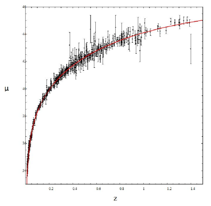
Figure 1: The distance modulus diagram for the best fit (red solid line) of the parameter of the Brane-Chern-Simons massive gravity theory in comparison with the 557 Union2 SNIa data points (black dots).

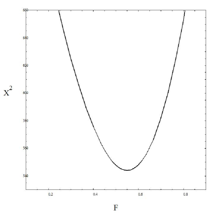
Figure 2: The $X^{2}$ functions of parameter $F$ for the Brane-Chern-Simons massive gravity theory.

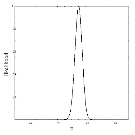
Figure 3: The likelihood as functions of parameter $F$ for the Brane-Chern-Simons massive gravity theory.

According to Figures 1 and 3, the result of fitting the Brane-Chern-Simons massive gravity theory to the cosmological data provides us with the optimal value for the model parameter.

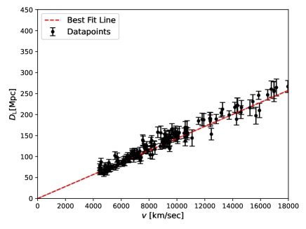
Figure 4: The best-fit diagram for the luminosity distance $D_{L}$ with respect to velocity $V$ for the Brane-Chern-Simons massive gravity theory.

To evaluate the validity of this theory, we utilize the Union2 supernovae Ia dataset, consisting of $557$ SNIa events. By employing the Bayesian statistics method, we constrain the model parameters based on the SNIa data. Specifically, we generate plots of $X^{2}$ and the likelihood function as functions of the parameter $F$, allowing us to determine the best-fit value by minimizing $X^{2}$.

Our analysis yields a best-fit value of $F=0.5497$ corresponding to a minimum $X^{2}$ value of $544.044$. Using this optimal parameter value, we calculate the best-fit value of $\mathcal{H}$ for the theory, obtaining $\mathcal{H}=0.6986$.

Figure 1 illustrates the distance modulus diagram, depicting the relationship between the distance modulus $\mu$ and the redshift $z$, along with the best-fit curve for the Brane-Chern-Simons massive gravity theory based on supernovae Ia data. Additionally, we provide a plot of velocity $V$ versus luminosity distance $D_{L}$, demonstrating the agreement between theoretical predictions and supernovae Ia observations. In Figure 4, we present a plot of the velocity $V$ as a function of luminosity distance $D_{L}$ for the Brane-Chern-Simons massive gravity theory. The velocity is calculated from the redshift using the equation $V=c-\frac{2c}{(z+1)^{2}+1}$.

5 Conclusion

In this work, we introduce a novel extension of massive gravity theory, the Brane-Chern-Simons massive gravity theory. We explore its potential to explain the late-time acceleration of the universe by deriving the full set of equations of motion for an FLRW background and analyzing self-accelerating background solutions. A key finding is the identification of self-accelerating solutions characterized by an effective cosmological constant, $\Lambda_{\rm SA}^{\pm}$. These solutions exhibit well-behaved behavior without strong coupling issues, offering a promising framework to explain the accelerated expansion of the universe.

Furthermore, our analysis of tensor perturbations provides insights into the nature of the graviton mass within this theory, leading to the derivation of the dispersion relation for gravitational waves. We also examine the stability of long-wavelength gravitational waves, where the sign of the mass square plays a crucial role. A positive mass square indicates stability, while a negative value suggests the presence of tachyons. However, the development of any instability due to tachyonic behavior is mitigated by the long timescales associated with the Hubble scale.

The validation of our model is demonstrated in the final section through a comparison with the latest Union2 SNIa dataset, consisting of 557 supernovae events. The Brane-Chern-Simons massive gravity theory exhibits an excellent fit with the observational data, as illustrated in Fig. 1. This allows us to constrain the model parameters and obtain a best-fit value of $\mathcal{H}=0.6986$ for the Hubble parameter, reinforcing the theory’s capability to describe the late-time acceleration of the universe. Future studies, utilizing larger and more diverse datasets, will be crucial for further refining and validating these findings, ultimately advancing our understanding of the fundamental principles governing the universe’s behavior.

Note added.

This is also a good position for notes added after the paper has been written.

References

- (1) S. Weinberg, Rev. Mod. Phys. 61 (1989), 1-23 doi:10.1103/RevModPhys.61.1
- (2) P. J. E. Peebles and B. Ratra, Rev. Mod. Phys. 75 (2003), 559-606 doi:10.1103/RevModPhys.75.559 [arXiv:astro-ph/0207347 [astro-ph]].
- (3) E. J. Copeland, M. Sami and S. Tsujikawa, Int. J. Mod. Phys. D 15 (2006), 1753-1936 doi:10.1142/S021827180600942X [arXiv:hep-th/0603057 [hep-th]].
- (4) S. M. Carroll, M. Hoffman and M. Trodden, Phys. Rev. D 68 (2003), 023509 doi:10.1103/PhysRevD.68.023509 [arXiv:astro-ph/0301273 [astro-ph]].
- (5) Y. F. Cai, E. N. Saridakis, M. R. Setare and J. Q. Xia, Phys. Rept. 493 (2010), 1-60 doi:10.1016/j.physrep.2010.04.001 [arXiv:0909.2776 [hep-th]].
- (6) K. Bamba, S. Capozziello, S. Nojiri and S. D. Odintsov, Astrophys. Space Sci. 342 (2012), 155-228 doi:10.1007/s10509-012-1181-8 [arXiv:1205.3421 [gr-qc]].
- (7) S. Nojiri and S. D. Odintsov, Phys. Rept. 505 (2011), 59-144 doi:10.1016/j.physrep.2011.04.001 [arXiv:1011.0544 [gr-qc]].
- (8) T. Clifton, P. G. Ferreira, A. Padilla and C. Skordis, Phys. Rept. 513 (2012), 1-189 doi:10.1016/j.physrep.2012.01.001 [arXiv:1106.2476 [astro-ph.CO]].
- (9) E. N. Saridakis et al. [CANTATA], Springer, 2021, ISBN 978-3-030-83714-3, 978-3-030-83717-4, 978-3-030-83715-0 doi:10.1007/978-3-030-83715-0 [arXiv:2105.12582 [gr-qc]].
- (10) M. Ishak, Living Rev. Rel. 22 (2019) no.1, 1 doi:10.1007/s41114-018-0017-4 [arXiv:1806.10122 [astro-ph.CO]].
- (11) E. Abdalla, G. Franco Abellán, A. Aboubrahim, A. Agnello, O. Akarsu, Y. Akrami, G. Alestas, D. Aloni, L. Amendola and L. A. Anchordoqui, et al. JHEAp 34 (2022), 49-211 doi:10.1016/j.jheap.2022.04.002 [arXiv:2203.06142 [astro-ph.CO]].
- (12) A. A. Starobinsky, Phys. Lett. B 91 (1980), 99-102 doi:10.1016/0370-2693(80)90670-X
- (13) S. Nojiri and S. D. Odintsov, Phys. Lett. B 631 (2005), 1-6 doi:10.1016/j.physletb.2005.10.010 [arXiv:hep-th/0508049 [hep-th]].
- (14) C. Erices, E. Papantonopoulos and E. N. Saridakis, Phys. Rev. D 99 (2019) no.12, 123527 doi:10.1103/PhysRevD.99.123527 [arXiv:1903.11128 [gr-qc]].
- (15) D. Lovelock, J. Math. Phys. 12 (1971), 498-501 doi:10.1063/1.1665613
- (16) G. W. Horndeski, Int. J. Theor. Phys. 10 (1974), 363-384 doi:10.1007/BF01807638
- (17) C. Deffayet, G. Esposito-Farese and A. Vikman, Phys. Rev. D 79 (2009), 084003 doi:10.1103/PhysRevD.79.084003 [arXiv:0901.1314 [hep-th]].
- (18) G. R. Bengochea and R. Ferraro, Phys. Rev. D 79 (2009), 124019 doi:10.1103/PhysRevD.79.124019 [arXiv:0812.1205 [astro-ph]].
- (19) Y. F. Cai, S. Capozziello, M. De Laurentis and E. N. Saridakis, Rept. Prog. Phys. 79 (2016) no.10, 106901 doi:10.1088/0034-4885/79/10/106901 [arXiv:1511.07586 [gr-qc]].
- (20) G. Kofinas and E. N. Saridakis, Phys. Rev. D 90 (2014), 084044 doi:10.1103/PhysRevD.90.084044 [arXiv:1404.2249 [gr-qc]].
- (21) S. Bahamonde, C. G. Böhmer and M. Wright, Phys. Rev. D 92 (2015) no.10, 104042 doi:10.1103/PhysRevD.92.104042 [arXiv:1508.05120 [gr-qc]].
- (22) C. Q. Geng, C. C. Lee, E. N. Saridakis and Y. P. Wu, Phys. Lett. B 704 (2011), 384-387 doi:10.1016/j.physletb.2011.09.082 [arXiv:1109.1092 [hep-th]].
- (23) K. Hinterbichler, Rev. Mod. Phys. 84 (2012), 671-710 doi:10.1103/RevModPhys.84.671 [arXiv:1105.3735 [hep-th]].
- (24) S. F. Hassan and R. A. Rosen, Phys. Rev. Lett. 108 (2012), 041101 doi:10.1103/PhysRevLett.108.041101 [arXiv:1106.3344 [hep-th]].
- (25) S. F. Hassan and R. A. Rosen, JHEP 02 (2012), 126 doi:10.1007/JHEP02(2012)126 [arXiv:1109.3515 [hep-th]].
- (26) C. de Rham and G. Gabadadze, Phys. Rev. D 82 (2010), 044020 doi:10.1103/PhysRevD.82.044020 [arXiv:1007.0443 [hep-th]].
- (27) C. de Rham, G. Gabadadze and A. J. Tolley, Phys. Rev. Lett. 106 (2011), 231101 doi:10.1103/PhysRevLett.106.231101 [arXiv:1011.1232 [hep-th]].
- (28) M. Fierz and W. Pauli, Proc. Roy. Soc. Lond. A 173 (1939), 211-232 doi:10.1098/rspa.1939.0140
- (29) H. van Dam and M. J. G. Veltman, Nucl. Phys. B 22 (1970), 397-411 doi:10.1016/0550-3213(70)90416-5
- (30) V. I. Zakharov, JETP Lett. 12 (1970), 312
- (31) A. I. Vainshtein, Phys. Lett. B 39 (1972), 393-394 doi:10.1016/0370-2693(72)90147-5
- (32) D. G. Boulware and S. Deser, Phys. Rev. D 6 (1972), 3368-3382 doi:10.1103/PhysRevD.6.3368
- (33) A. De Felice, A. E. Gumrukcuoglu and S. Mukohyama, Phys. Rev. Lett. 109 (2012), 171101 doi:10.1103/PhysRevLett.109.171101 [arXiv:1206.2080 [hep-th]].
- (34) A. E. Gumrukcuoglu, C. Lin and S. Mukohyama, JCAP 03 (2012), 006 doi:10.1088/1475-7516/2012/03/006 [arXiv:1111.4107 [hep-th]].
- (35) G. D’Amico, G. Gabadadze, L. Hui and D. Pirtskhalava, Phys. Rev. D 87 (2013), 064037 doi:10.1103/PhysRevD.87.064037 [arXiv:1206.4253 [hep-th]].
- (36) R. Gannouji, M. W. Hossain, M. Sami and E. N. Saridakis, Phys. Rev. D 87 (2013), 123536 doi:10.1103/PhysRevD.87.123536 [arXiv:1304.5095 [gr-qc]].
- (37) A. De Felice, A. Emir Gümrükçüoğlu and S. Mukohyama, Phys. Rev. D 88 (2013) no.12, 124006 doi:10.1103/PhysRevD.88.124006 [arXiv:1309.3162 [hep-th]].
- (38) S. Mukohyama, JCAP 12 (2014), 011 doi:10.1088/1475-7516/2014/12/011 [arXiv:1410.1996 [hep-th]].
- (39) N. Tamanini, E. N. Saridakis and T. S. Koivisto, JCAP 02 (2014), 015 doi:10.1088/1475-7516/2014/02/015 [arXiv:1307.5984 [hep-th]].
- (40) A. Emir Gümrükçüoğlu, L. Heisenberg and S. Mukohyama, JCAP 02 (2015), 022 doi:10.1088/1475-7516/2015/02/022 [arXiv:1409.7260 [hep-th]].
- (41) Y. F. Cai, F. Duplessis and E. N. Saridakis, Phys. Rev. D 90 (2014) no.6, 064051 doi:10.1103/PhysRevD.90.064051 [arXiv:1307.7150 [hep-th]].
- (42) T. Kahniashvili, A. Kar, G. Lavrelashvili, N. Agarwal, L. Heisenberg and A. Kosowsky, Phys. Rev. D 91 (2015) no.4, 041301 [erratum: Phys. Rev. D 100 (2019) no.8, 089902] doi:10.1103/PhysRevD.91.041301 [arXiv:1412.4300 [astro-ph.CO]].
- (43) Y. F. Cai and E. N. Saridakis, Phys. Rev. D 90 (2014) no.6, 063528 doi:10.1103/PhysRevD.90.063528 [arXiv:1401.4418 [astro-ph.CO]].
- (44) A. E. Gumrukcuoglu, K. Koyama and S. Mukohyama, Phys. Rev. D 94 (2016) no.12, 123510 doi:10.1103/PhysRevD.94.123510 [arXiv:1610.03562 [hep-th]].
- (45) A. E. Gumrukcuoglu, K. Koyama and S. Mukohyama, Phys. Rev. D 96 (2017) no.4, 044041 doi:10.1103/PhysRevD.96.044041 [arXiv:1707.02004 [hep-th]].
- (46) A. E. Gumrukcuoglu, R. Kimura and K. Koyama, Phys. Rev. D 101 (2020) no.12, 124021 doi:10.1103/PhysRevD.101.124021 [arXiv:2003.11831 [gr-qc]].
- (47) A. De Felice, S. Mukohyama and M. C. Pookkillath, JCAP 12 (2021) no.12, 011 doi:10.1088/1475-7516/2021/12/011 [arXiv:2110.01237 [astro-ph.CO]].
- (48) A. R. Akbarieh, S. Kazempour and L. Shao, Phys. Rev. D 103 (2021), 123518 doi:10.1103/PhysRevD.103.123518 [arXiv:2105.03744 [gr-qc]].
- (49) A. R. Akbarieh, S. Kazempour and L. Shao, Phys. Rev. D 105 (2022) no.2, 023501 doi:10.1103/PhysRevD.105.023501 [arXiv:2203.00901 [gr-qc]].
- (50) S. Kazempour and A. R. Akbarieh, Phys. Rev. D 105 (2022) no.12, 123515 doi:10.1103/PhysRevD.105.123515 [arXiv:2204.05595 [gr-qc]].
- (51) S. Kazempour, A. R. Akbarieh, H. Motavalli and L. Shao, Phys. Rev. D 106 (2022) no.2, 023508 doi:10.1103/PhysRevD.106.023508 [arXiv:2205.10863 [gr-qc]].
- (52) S. Kazempour, A. R. Akbarieh and E. N. Saridakis, Phys. Rev. D 106 (2022) no.10, 103502 doi:10.1103/PhysRevD.106.103502 [arXiv:2207.13936 [gr-qc]].
- (53) A. E. Gümrükçüoğlu, K. Hinterbichler, C. Lin, S. Mukohyama and M. Trodden, Phys. Rev. D 88 (2013) no.2, 024023 doi:10.1103/PhysRevD.88.024023 [arXiv:1304.0449 [hep-th]].
- (54) Z. Haghani, H. R. Sepangi and S. Shahidi, Phys. Rev. D 87 (2013) no.12, 124014 doi:10.1103/PhysRevD.87.124014 [arXiv:1303.2843 [gr-qc]].
- (55) G. D’Amico, G. Gabadadze, L. Hui and D. Pirtskhalava, Class. Quant. Grav. 30 (2013), 184005 doi:10.1088/0264-9381/30/18/184005 [arXiv:1304.0723 [hep-th]].
- (56) F. Izaurieta, E. Rodriguez, P. Minning, P. Salgado and A. Perez, Phys. Lett. B 678 (2009), 213-217 doi:10.1016/j.physletb.2009.06.017 [arXiv:0905.2187 [hep-th]].
- (57) F. Gómez, S. Lepe and P. Salgado, Eur. Phys. J. C 81 (2021) no.1, 9 doi:10.1140/epjc/s10052-020-08804-z [arXiv:2012.10578 [gr-qc]].
- (58) P. K. Concha, R. Durka, C. Inostroza, N. Merino and E. K. Rodríguez, Phys. Rev. D 94 (2016) no.2, 024055 doi:10.1103/PhysRevD.94.024055 [arXiv:1603.09424 [hep-th]].
- (59) F. Gomez, P. Minning and P. Salgado, Phys. Rev. D 84 (2011), 063506 doi:10.1103/PhysRevD.84.063506
- (60) S. Nojiri, S. D. Odintsov, V. K. Oikonomou and A. A. Popov, Phys. Rev. D 100 (2019) no.8, 084009 doi:10.1103/PhysRevD.100.084009 [arXiv:1909.01324 [gr-qc]].
- (61) S. D. Odintsov and V. K. Oikonomou, Phys. Rev. D 105 (2022) no.10, 104054 doi:10.1103/PhysRevD.105.104054 [arXiv:2205.07304 [gr-qc]].
- (62) S. Nojiri, S. D. Odintsov, V. K. Oikonomou and A. A. Popov, Phys. Dark Univ. 28 (2020), 100514 doi:10.1016/j.dark.2020.100514 [arXiv:2002.10402 [gr-qc]].
- (63) P. K. Concha, D. M. Penafiel, E. K. Rodriguez and P. Salgado, Eur. Phys. J. C 74 (2014), 2741 doi:10.1140/epjc/s10052-014-2741-6 [arXiv:1402.0023 [hep-th]].
- (64) M. A. Scheel, S. L. Shapiro and S. A. Teukolsky, Phys. Rev. D 51 (1995), 4208-4235 doi:10.1103/PhysRevD.51.4208 [arXiv:gr-qc/9411025 [gr-qc]].
- (65) T. Christodoulakis, N. Dimakis and P. A. Terzis, J. Phys. A 47 (2014), 095202 doi:10.1088/1751-8113/47/9/095202 [arXiv:1304.4359 [gr-qc]].
- (66) N. Arkani-Hamed, H. Georgi and M. D. Schwartz, Annals Phys. 305 (2003), 96-118 doi:10.1016/S0003-4916(03)00068-X [arXiv:hep-th/0210184 [hep-th]].
- (67) C. Grosse-Knetter and R. Kogerler, Phys. Rev. D 48 (1993), 2865-2876 doi:10.1103/PhysRevD.48.2865 [arXiv:hep-ph/9212268 [hep-ph]].
- (68) J. Frieman, M. Turner and D. Huterer, Ann. Rev. Astron. Astrophys. 46 (2008), 385-432 doi:10.1146/annurev.astro.46.060407.145243 [arXiv:0803.0982 [astro-ph]].
- (69) S. Perlmutter and B. P. Schmidt, Lect. Notes Phys. 598 (2003), 195-217 doi:10.1007/3-540-45863-8_11 [arXiv:astro-ph/0303428 [astro-ph]].
- (70) Y. Yang and Y. Gong, JCAP 06 (2020), 059 doi:10.1088/1475-7516/2020/06/059 [arXiv:1912.07375 [astro-ph.CO]].
- (71) R. Amanullah, C. Lidman, D. Rubin, G. Aldering, P. Astier, K. Barbary, M. S. Burns, A. Conley, K. S. Dawson and S. E. Deustua, et al. Astrophys. J. 716 (2010), 712-738 doi:10.1088/0004-637X/716/1/712 [arXiv:1004.1711 [astro-ph.CO]].
- (72) S. Nesseris and L. Perivolaropoulos, Phys. Rev. D 72 (2005), 123519 doi:10.1103/PhysRevD.72.123519 [arXiv:astro-ph/0511040 [astro-ph]].
- (73) E. Di Pietro and J. F. Claeskens, Mon. Not. Roy. Astron. Soc. 341 (2003), 1299 doi:10.1046/j.1365-8711.2003.06508.x [arXiv:astro-ph/0207332 [astro-ph]].