Domar aggregation under nonneutral elasticity of substitution

Abstract

The characteristics inherent in a Domar aggregation, when all sectoral productions embody a common nonneutral elasticity of substitution, is examined. There, the general equilibrium propagation of productivity changes entails structural transformation that brings nonlinearities in their aggregation into price indices. We show that negative singularity, such that a finite productivity decrease induces an infinitely large price, is possible in an inelastic economy, while positive singularity, such that a finite productivity increase induces a zero price, is possible in an elastic economy. Regarding the aggregate outputs, two independent productivity changes will have synergism in an elastic economy, whereas negative synergism will be prevalent in an inelastic economy. Neither issue is of concern in a Cobb-Douglas economy where the elasticity of substitution is everywhere neutral.

C67 D51 O41

1 Introduction

In this paper, we are concerned with the practice of evaluating technological innovations. In economics terminology, the level of technology of an industry corresponds to its productivity, thus innovation to its growth, and the evaluation corresponds to the assessment of potential impact that productivity growth may deliver into the aggregate output of an economy, or more specifically, the GDP growth. One such thing that aggregates sectoral productivity growths into GDP growth is known as the Domar aggregator. Hulten (1978) claimed that the impact on aggregate output can be assessed as a linear combination of sector-level productivity shocks with coefficients given by sectors’ Domar weights. Under the general equilibrium framework comprising Cobb-Douglas technologies throughout, Domar weights turns out to be the final expenditure share weighted sum of the Leontief inverse.

Accordingly, Acemoglu et al (2012, 2017); Acemoglu and Azar (2020) study linear Domar aggregation whereby assuming neutral elasticity of substitution in all sectoral productions as well as in the households’ final consumption, and focus on the effect of granularity (Gabaix, 2011) inherent in the network of input-output linkages. Meanwhile, Baqaee and Farhi (2019) study aggregate fluctuations on the basis of second-order approximation of nonlinear Domar aggregation. Kim et al (2017); Nakano and Nishimura (2024) study the characteristics of empirical Domar aggregation based on a system of sector-specific CES unit cost functions where every equilibrium is reached numerically by recursive contraction. It is now obvious that the elasticity of substitution in all sectoral productions is essential in defining the characteristics of Domar aggregations.

Nonneutrality of the elasticities, however, prevents our system of equations that equilibriates sectoral unit costs with commodity prices from being linear. We therefore simplify the matter first by allowing nonneutral but unitary elasticity of substitution in all sectors’ CES unit cost functions. This assumption turns our nonlinear system of equations with respect to normal prices into a linear system of equations with respect to hyperprices. Readily, the equilibrium hyperprices can be solved by way of linear algebra. We then take the advantage of our knowledge about the viability of input-output matrices, to study the consequences of singularity that can potentially be established in the hyperstructure. Our approach enables to analytically examine not only singularity but also synergism among innovations, with respect to the elasticity of substitution.

The rest of the paper is organized as follows. In the following section, we specify the model of an economy comprised of multiple CES aggregator functions of unitary elasticity of substitution, and derive the Domar aggregation function with respect to the (exogenous) productivity changes and the underlying elasticity of substitution. Our approach to model multisector general equilibrium in the hyperspace enables us to handle equilibrium solutions by means of linear algebra. In section 3, we discuss the matter of singularity, and specify the conditions whereby such a phenomenon is possible. We find that inelastic (elastic) economy may encounter a negative (positive) singularity. In section 4, we discuss the matter of synergism in the economic evaluation of innovation(s). We find that an inelastic (elastic) economy entails negative (positive) synergism. Section 5 concludes the paper.

2 The model

2.1 Production

We write down below a CES production of constant returns to scale, and the corresponding unit cost function for the $j$th industry (index suppressed), with $i=1,\cdots,n$ being an intermediate factor input, and $i=0$ being a sigle primary factor of production.

$${x}={z}\left(\sum_{i=0}^{n}({\alpha}_{i})^{\frac{1}{\sigma}}({x}_{i})^{\frac{\sigma-1}{\sigma}}\right)^{\frac{\sigma}{\sigma-1}}, {p}={z}^{-1}\left(\sum_{i=0}^{n}{\alpha}_{i}({p}_{i})^{1-\sigma}\right)^{\frac{1}{1-\sigma}}$$ (1)

Here, elasticity of substitution is denoted by $\sigma$. The share parameter is denoted by $\alpha_{i}$, and assumed that $\sum_{i=0}^{n}\alpha_{i}=1$. Quantities and prices are denoted by $x$ and $p$, respectively. The Hickes-neutral productivity level of the industry is denoted by $z$. Note that duality asserts zero profit, i.e., $px=\sum_{i=0}^{n}p_{i}x_{i}$.

The (quasi-) concavity of the production function is assured if $\sigma>0$. Note that $\sigma=0$ corresponds to Leontief production, while $\sigma=1$ corresponds to Cobb-Douglas, the case of which we call neutral elasticity of substitution. Application of Shepahrd’s lemma to the unit cost function (1 right) yeilds the following:

$$s_{i}\equiv\frac{x_{i}}{x}\frac{p_{i}}{p}=\frac{\partial p}{\partial p_{i}}\frac{p_{i}}{p}={\alpha}_{i}\left(\frac{p_{i}}{zp}\right)^{1-\sigma}$$ (2)

That is, for the case of Cobb-Douglas production ($\sigma=1$) the cost share $s_{i}$ is unaffected by the changes in productivity and/or prices and stays at $\alpha_{i}$. Moreover, a Cobb-Douglas unit cost function becomes log-linear by the following expansion of (1 right) where ${\gamma}=1-{\sigma}$:

$$\ln zp=\lim_{\gamma\to 0}\frac{\ln\left(\sum_{i=0}^{n}\alpha_{i}(p_{i})^{\gamma}\right)}{\gamma}=\lim_{\gamma\to 0}\frac{\sum_{i=0}^{n}\alpha_{i}(p_{i})^{\gamma}\ln p_{i}}{\sum_{i=0}^{n}\alpha_{i}(p_{i})^{\gamma}}=\sum_{i=0}^{n}\alpha_{i}\ln p_{i}$$ (3)

Here, l’Hôspital’s rule with the assumption that $\sum_{i=0}^{n}\alpha_{i}=1$ is used.

Taking the $\gamma$th power on both sides of the unit cost function (1 right) yields:

$${p}^{\gamma}={z}^{-\gamma}\left({\alpha}_{1}({p}_{1})^{\gamma}+{\alpha}_{2}({p}_{2})^{\gamma}+\cdots+{\alpha}_{n}({p}_{n})^{\gamma}+{\alpha}_{0}({p}_{0})^{\gamma}\right)$$ (4)

Consider the following $n$-industry general equilibrium model comprised of CES unit cost functions all with the same elasticity of substitution $\sigma=1-\gamma$:

$$\begin{aligned} ({p}_{1})^{\gamma}&=({z}_{1})^{-{\gamma}}\left({\alpha}_{11}({p}_{1})^{\gamma}+{\alpha}_{21}({p}_{2})^{\gamma}+\cdots+{\alpha}_{{n}1}({p}_{n})^{\gamma}+{\alpha}_{01}({p}_{0})^{\gamma}\right)\\ ({p}_{2})^{\gamma}&=({z}_{2})^{-{\gamma}}\left({\alpha}_{12}({p}_{1})^{\gamma}+{\alpha}_{22}({p}_{2})^{\gamma}+\cdots+{\alpha}_{{n}2}({p}_{n})^{\gamma}+{\alpha}_{02}({p}_{0})^{\gamma}\right)\\ \vdots&\\ ({p}_{n})^{\gamma}&=({z}_{n})^{-{\gamma}}\left({\alpha}_{1n}({p}_{1})^{\gamma}+{\alpha}_{2n}({p}_{2})^{\gamma}+\cdots+{\alpha}_{{n}n}({p}_{n})^{\gamma}+{\alpha}_{0n}({p}_{0})^{\gamma}\right)\end{aligned}$$ (5)

Let us call hereafter the case with $\gamma=1-\sigma<0$ an elastic economy, $\gamma=1-\sigma>0$ an inelastic economy, and the case with $\gamma=1-\sigma=0$ a Cobb-Douglas, or neutrally elastic economy. In any case, we may analytically solve for the hyperprice ${\phi}_{j}\equiv({p}_{j})^{\gamma}>0$ as a function of hyperproductivity ${\zeta}_{j}\equiv({z}_{j})^{-\gamma}>0$, for $j=1,\cdots,n$, as follows:

$$\boldsymbol{\phi}=\left[\mathbf{I}-\left<\boldsymbol{\zeta}\right>\mathbf{A}\right]^{-1}\left<\boldsymbol{\zeta}\right>\boldsymbol{\alpha}_{0}$$ (6)

where, $\boldsymbol{\zeta}=({\zeta}_{1},\cdots,{\zeta}_{n})$, $\boldsymbol{\phi}=({\phi}_{1},\cdots,{\phi}_{n})^{\prime}$, $\boldsymbol{\alpha}_{0}=({\alpha}_{01},\cdots,{\alpha}_{0n})^{\prime}$, and $\mathbf{A}=[{\alpha}_{ij}]^{\prime}$.Angle brackets indicate vector diagonalization. The price of primary factor is reserved as the numéraire, i.e., $p_{0}=1$. Commodity prices are denoted as $\boldsymbol{p}=({p}_{1},{p}_{2},\cdots,{p}_{n})$. We normalize prices, i.e., set $\boldsymbol{\phi}=\boldsymbol{p}=(1,1,\cdots,1)^{\prime}=\boldsymbol{1}$, at the baseline where $\boldsymbol{\zeta}=\boldsymbol{z}=\boldsymbol{1}$. In this event, cost share matrix $\mathbf{S}=[s_{ij}]^{\prime}$ must be identicdal to $\mathbf{A}$ according to (2). Moreover,

$$\boldsymbol{1}=\left[\mathbf{I}-\mathbf{A}\right]^{-1}\boldsymbol{\alpha}_{0}>0$$ (7)

2.2 Household

Below are a representative household’s (indirect) utility function of CES, and the corresponding (consumer’s) price index:

$${U}=\left(\sum_{i=1}^{n}({\mu}_{i})^{\frac{1}{\eta}}({c}_{i})^{\frac{{\eta}-1}{\eta}}\right)^{\frac{\eta}{{\eta}-1}}, {I}(\boldsymbol{p})=\left(\sum_{i=1}^{n}{\mu}_{i}({p}_{i})^{1-{\eta}}\right)^{\frac{1}{1-{\eta}}}$$

where the indirect utility and consumer’s price index are denoted by ${U}$ and ${I}$, respectively. The representative household’s consumption shcedule in physical terms is denoted by $\boldsymbol{c}=({c}_{1},{c}_{2},\cdots,{c}_{n})$, while its elasticity of substitution among the commodities is denoted by ${\eta}$. The share parameter ${\mu}_{i}$ is subject to the constraint $\sum_{i=1}^{n}{\mu}_{i}=1$. Because ${B}\equiv{U}{I}=\sum_{i=1}^{n}{p}_{i}{c}_{i}$, ${B}$ implies the GDE (gross domestic expenditure) which equals the GDP (gross domestic product) and the GDI (gross domestic income) or total value added.

Consider the baseline (state of origin) where all prices are normalized at unity, i.e., $\boldsymbol{p}=\boldsymbol{1}=(1,1,\cdots,1)^{\prime}$. At the baseline, ${B}={U}$, because ${I}(\boldsymbol{1})=1$. Given the price change, ${B}={U}{I}(\boldsymbol{p})$ indicates that $U$ is the real GDP if $W$ is the nominal GDP, while $I(\boldsymbol{p})$ being the GDP deflator. As we normalize the nominal GDP at unity (${B}=1$), and assuming Cobb-Douglas utility (${\eta}\to 1$) the aggregate output growth $\ln U$ can be evaluated as follows:

$$\ln{U}=\ln{B}-\ln I(\boldsymbol{p})=-\ln I(\boldsymbol{p})=-\sum_{i=1}^{n}{\mu}_{i}\ln{p}_{i}=-\boldsymbol{\mu}\ln\boldsymbol{p}$$ (8)

Note that the third identity is evident by the analogy from (3).

2.3 Domar aggregation

An approach to aggregating growth measures associated with industries (as such of productivity growths $\ln\boldsymbol{z}=(\ln{z}_{1},\ln{z}_{2},\cdots,\ln{z}_{n})$) to national aggregate growth (as such of real GDP growth $\ln U$) is called a Domar aggregation. For sake of simplicity, let us assume hereafter that utility is Cobb-Douglas, i.e., ${\eta}=1$. This allows the real GDP growth to be the weighted sum of price growths as specified in (8). With regard to (6), the hyperspace Domar aggregator can be specified as follows:

$$-\boldsymbol{\mu}\ln\boldsymbol{\phi}=-\boldsymbol{\mu}{\gamma}\ln\boldsymbol{p}={\gamma}\ln{U}=-\boldsymbol{\mu}\ln\left(\left[\mathbf{I}-\left<\boldsymbol{\zeta}\right>\mathbf{A}\right]^{-1}\left<\boldsymbol{\zeta}\right>\boldsymbol{\alpha}_{0}\right)$$

Accordingly, the Domar aggregator that aggregates sectoral productivity growths $\ln\boldsymbol{z}$ into real GDP growth $\ln{U}$ under an unitary substitution elasticity ${\sigma}=1-{\gamma}$ be as follows:

$$\ln U=-\left(\boldsymbol{\mu}/{\gamma}\right)\ln\left(\left[\mathbf{I}-\left<e^{-\gamma\ln\boldsymbol{z}}\right>\mathbf{A}\right]^{-1}\left<e^{-\gamma\ln\boldsymbol{z}}\right>\boldsymbol{\alpha}_{0}\right)$$

For the case of Cobb-Douglas production ($\gamma\to 0$), price growths have the following interdependences, according to (3),

$$\ln{p}_{1}+\ln{z}_{1} ={\alpha}_{11}\ln{p}_{1}+{\alpha}_{21}\ln{p}_{2}+\cdots+{\alpha}_{{n}1}\ln{p}_{n}$$

$$\ln{p}_{2}+\ln{z}_{2} ={\alpha}_{12}\ln{p}_{1}+{\alpha}_{22}\ln{p}_{2}+\cdots+{\alpha}_{{n}2}\ln{p}_{n}$$

$$\vdots$$

$$\ln{p}_{n}+\ln{z}_{n} ={\alpha}_{1n}\ln{p}_{1}+{\alpha}_{2n}\ln{p}_{2}+\cdots+{\alpha}_{{n}{n}}\ln{p}_{n}$$

where the equilibrium price can be solved as follows:

$$\ln\boldsymbol{p}=\left[\mathbf{I}-\mathbf{A}\right]^{-1}\ln\boldsymbol{z}$$ (9)

Thus, the Domar aggregator for a Cobb-Douglas (elasticity-neutral) economy (with ${\eta}={\sigma}=1$) can be specified as follows:

$$\ln U=-\boldsymbol{\mu}\ln\boldsymbol{p}=\boldsymbol{\mu}\left[\mathbf{I}-\mathbf{A}\right]^{-1}\ln\boldsymbol{z}$$

In other words, the households’ expenditure share-weighted Leontief inverse becomes the Domar weights.

3 Singularity

3.1 Two-sector general equilibrium

Let us herewith consider a two-sector general equilibrium comprised of two CES unit cost functions with unitary elasticity of substitution in the form of (5), as follows:

$$({p}_{1})^{\gamma} =({z}_{1})^{-{\gamma}}\left({\alpha}_{21}({p}_{2})^{\gamma}+{\alpha}_{01}\right)$$

$$({p}_{2})^{\gamma} =({z}_{2})^{-{\gamma}}\left({\alpha}_{12}({p}_{1})^{\gamma}+{\alpha}_{02}\right)$$

Here we assume that ${\alpha}_{11}={\alpha}_{22}=0$ for simplicity. The system of equations in the hyperspace is as follows:

$$\begin{bmatrix}[r]{\phi}_{1}\\ {\phi}_{2}\end{bmatrix}=\begin{bmatrix}[c]{\zeta}_{1}&0\\ 0&{\zeta}_{2}\end{bmatrix}\begin{bmatrix}[c]0&{\alpha}_{21}\\ {\alpha}_{12}&0\end{bmatrix}\begin{bmatrix}[r]{\phi}_{1}\\ {\phi}_{2}\end{bmatrix}+\begin{bmatrix}[c]{\zeta}_{1}&0\\ 0&{\zeta}_{2}\end{bmatrix}\begin{bmatrix}[r]{\alpha}_{01}\\ {\alpha}_{02}\end{bmatrix}$$

and hence we can solve for the hyper-price by way of (6), as follows:

$$\boldsymbol{\phi}=\left[\mathbf{I}-\left<\boldsymbol{\zeta}\right>\mathbf{A}\right]^{-1}\left<\boldsymbol{\zeta}\right>\boldsymbol{\alpha}_{0}=\frac{1}{1-{\alpha}_{21}{\alpha}_{12}{\zeta}_{1}{\zeta}_{2}}\begin{bmatrix}[r]{{\alpha}_{01}{\zeta}_{1}+{\alpha}_{21}{\zeta}_{1}{\alpha}_{02}{\zeta}_{2}}\\ {{\alpha}_{02}{\zeta}_{2}+{\alpha}_{12}{\zeta}_{2}{\alpha}_{01}{\zeta}_{1}}\end{bmatrix}$$

According to Hawkins and Simon (1949)’s theory, following nonsingularity condition must be met in order for the equilibrium hyperprices to be positive, i.e., $\boldsymbol{\phi}>0$, for any possible change of hyperproductivities, i.e., $\left<\boldsymbol{\zeta}\right>\boldsymbol{\alpha}_{0}>0$.

$$D=\det\left(\mathbf{I}-\left<\boldsymbol{\zeta}\right>\mathbf{A}\right)=1-{\alpha}_{21}{\alpha}_{12}{\zeta}_{1}{\zeta}_{2}>0$$ (10)

At the same time, we know that hyperprices approach infinity, i.e., $\boldsymbol{\phi}\to\infty$, as the hyperstructure of the economy approaches singularity, i.e., $D\to 0$. Figure 1 depicts a sample contour plot of the determinant $D$ with respect to productivity change $({z}_{1},{z}_{2})$, where we display the function below:

$$D=1-{\alpha}_{21}{\alpha}_{12}({z}_{1}{z}_{2})^{\gamma}$$ (11)

Note that Figure 1 depicts the case of inelastic economy ${\gamma}>0$ on the left, and the case of elastic economy ${\gamma}<0$ on the right. The point is that productivity decline in an inelastic economy or productivity increase in an elastic economy brings the hyper-structure towards singularity.

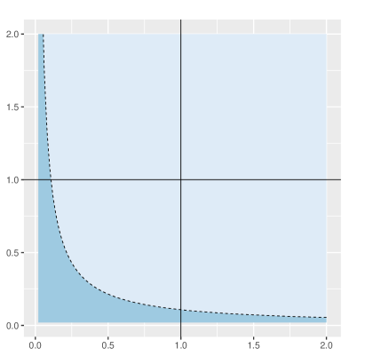
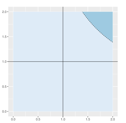
Figure 1: Contour plots of (11) where the horizontal and vertical axis correspond to ${z}_{1}$ and ${z}_{2}$, respectively. The left figure corresponds to an inelastic economy ($\gamma=0.1$, ${\alpha}_{21}{\alpha}_{12}=0.8$), and the right to an elastic economy ($\gamma=-0.5$, ${\alpha}_{21}{\alpha}_{12}=0.6$). Dotted line indicates singularity where $D\to 0$. The dark areas indicate that $D<0$. Nonsingularity ($D>0$) is held at the state of origin $({z}_{1},{z}_{2})=(1,1)$ for both cases.

The outcome of singularity in the hyperstructure ($D\to 0$) also depends on the elasticity of substitution in all productions (${\sigma}=1-{\gamma}$). Specifically, because $\boldsymbol{\phi}\to\boldsymbol{\infty}$ as $D\to 0$,

$${p}_{j}=({\phi}_{j})^{1/\gamma}\to\begin{cases}~{}\infty&\text{~{}~{}\text{Inelastic }($0<\gamma<1$)}\\ ~{}0&\text{~{}~{}\text{Elastic }($\gamma<0$)}\end{cases} j=1,2$$

That is, singularity in the hyperstructure brings hyperprice to infinity, where the price approaches infinity in an inelastic economy, while towards zero in an elastic economy. We are also concerned about the physical requirement of the primary factor of production $i=0$ in all sectors in the neighborhood of hyperstructure singularity. Application of Shephard’s lemma onto each unit cost function yields the following:

$$b_{ij}\equiv\frac{x_{ij}}{x_{j}}=\frac{\partial p_{j}}{\partial p_{i}}={\alpha}_{ij}\left(\frac{p_{i}}{p_{j}}\right)^{-{\sigma}}({z}_{j})^{\sigma-1}={\alpha}_{ij}\left(\frac{{\phi}_{i}}{{\phi}_{j}}\right)^{1-{1/\gamma}}{\zeta}_{j}$$

where $b_{ij}$ denotes input-output coefficient in physical terms for $i=0,1,2$ and $j=1,2$. Since ${\phi}_{0}=1$, the primary factor input per unit output in physical terms be:

$$b_{0j}={\alpha}_{0j}({\phi}_{j})^{{1/\gamma}-1}{\zeta}_{j}=\begin{cases}~{}\infty&\text{~{}~{}\text{Inelastic}}\\ ~{}0&\text{~{}~{}\text{Elastic}}\end{cases} j=1,2$$

at the hyperstructure singularity where $\boldsymbol{\phi}\to\boldsymbol{\infty}$. That is, some finite productivity change ($\boldsymbol{0}<\boldsymbol{z}^{\gamma}=\boldsymbol{\zeta}\ll\boldsymbol{\infty}$) can bring the per-output requirement of primary factor to infinity in an inelastic economy, while towards zero in an elastic economy. Finally note that such an issue (price infinitely large or zero under the aegis of finite productivity change) will not be of concern in an elasticity-neutral (Cobb-Douglas) economy by the sake of (9).

3.2 Multisector general equilibrium

Hawkins and Simon (1949)’s claim can be interpreted that the following viability condition is equivalent to the existence of positive solution $\boldsymbol{\phi}>0$ for any $\left<\boldsymbol{\zeta}\right>\boldsymbol{a}_{0}>0$, regarding (6).

$$D_{k}=\det\left(\mathbf{I}-\left<\boldsymbol{\zeta}\right>\mathbf{A}\right)_{k}>0 k=1,2,\cdots,n$$ (12)

That is, all the successive (the $k$th) principal minor determinants of $[\mathbf{I}-\left<\boldsymbol{\zeta}\right>\mathbf{A}]$ must be positive. At the baseline ($\boldsymbol{\zeta}=\boldsymbol{1}$), this condition is met by the sake of (7). Also, we know by Nikaido (1968) that the following conditions are equivalent:

$$\det\left(\mathbf{I}-\mathbf{A}\right)_{k}>0, \lim_{t\to\infty}\left(\mathbf{A}_{k}\right)^{t}=0$$

Following Takayama (1985), let us confirm this for the $k$th minor (index omitted).

Let $\mathbf{M}_{T}\equiv\sum_{t=0}^{T}\mathbf{A}^{t}=\mathbf{I}+\mathbf{A}+\cdots+\mathbf{A}^{T}$, then

$$\mathbf{M}_{T}\left[\mathbf{I}-\mathbf{A}\right]=\mathbf{I}-\mathbf{A}^{T+1}=\left[\mathbf{I}-\mathbf{A}\right]\mathbf{M}_{T}$$ (13)

Since $\mathbf{A}>\boldsymbol{0}$, it must be that $\mathbf{A}^{T+1}>\boldsymbol{0}$, so that $\mathbf{I}>\left[\mathbf{I}-\mathbf{A}\right]\mathbf{M}_{T}$. The nonsingularity assumption of $[\mathbf{I}-\mathbf{A}]$ allows one to see that $M_{T}$ is bounded from above and increasing in $T$, as follows:

$$\mathbf{L}\equiv\left[\mathbf{I}-\mathbf{A}\right]^{-1}>\mathbf{M}_{T}>\mathbf{M}_{T-1}>\cdots>\mathbf{M}_{0}=\mathbf{I}>\boldsymbol{0}$$ (14)

By Hawkins and Simon (1949) we know this is equivalent to $\det(\mathbf{I}-\mathbf{A})_{k}>0$ for $k=1,\cdots,n$. Also, since the above exposition tells that $\mathbf{M}_{\infty}$ is convergent, it must be true that

$$\lim_{T\to\infty}\left(\mathbf{A}^{T+1}=\mathbf{M}_{T+1}-\mathbf{M}_{T}\right)=\boldsymbol{0}$$

Conversely, if $\mathbf{A}^{\infty}\to 0$, then we know that $\mathbf{L}=\mathbf{M}_{\infty}>0$ by (13), which we know is equivalent to (14). Therefore, $\mathbf{L}>\boldsymbol{0}$, $\det(\mathbf{I}-\mathbf{A})>0$ and $\mathbf{A}^{\infty}\to\boldsymbol{0}$ are all equivalent statements.

Hence, our purpose to show (12) amounts to showing that $\left(\left<\boldsymbol{\zeta}\right>\mathbf{A}\right)^{\infty}\to\boldsymbol{0}$. To do so, we first eigendecompose $\mathbf{A}$ which is a square, nonnegative and nonsingular matrix, for further evaluation of the hyperstructure, as follows:

$$\left<\boldsymbol{\zeta}\right>\mathbf{A}=\left<\boldsymbol{\zeta}\right>\mathbf{Q}\left<\boldsymbol{\lambda}\right>\mathbf{Q}^{-1}<\left({\zeta}_{\text{max}}\mathbf{I}\right)\mathbf{Q}\left<\boldsymbol{\lambda}\right>\mathbf{Q}^{-1}=\mathbf{Q}\left<{\zeta}_{\text{max}}\boldsymbol{\lambda}\right>\mathbf{Q}^{-1}$$

Here, $\left<\boldsymbol{\lambda}\right>$ denotes the diagonal matrix of the eigenvalues of $\mathbf{A}$, and ${\zeta}_{\text{max}}=\max_{j}\boldsymbol{\zeta}>0$ is a scalar. Because $\mathbf{A}^{\infty}\to\boldsymbol{0}$, we know that $\left<\boldsymbol{\lambda}\right>^{\infty}=\mathbf{Q}^{-1}\mathbf{A}^{\infty}\mathbf{Q}\to\boldsymbol{0}$. In other words $|{\lambda}_{j}|<1$ for $j=1,\cdots,n$. Thus, for any $\boldsymbol{\zeta}<\boldsymbol{1}$, it must be true that $|{\zeta}_{\text{max}}{\lambda}_{j}|<1$ for $j=1,\cdots,n$, so that nonsingularity of the hyperstructure is secured, i.e.,

$$\boldsymbol{0}<\left(\left<\boldsymbol{\zeta}\right>\mathbf{A}\right)^{\infty}<\mathbf{Q}\left<{\zeta}_{\text{max}}\boldsymbol{\lambda}\right>^{\infty}\mathbf{Q}^{-1}\to\boldsymbol{0} \forall\boldsymbol{\zeta}<\boldsymbol{1}$$

On the other hand, the hyperstructure can also be evaluated as follows:

$$\left<\boldsymbol{\zeta}\right>\mathbf{A}=\left<\boldsymbol{\zeta}\right>\mathbf{Q}\left<\boldsymbol{\lambda}\right>\mathbf{Q}^{-1}>\left({\zeta}_{\text{min}}\mathbf{I}\right)\mathbf{Q}\left<\boldsymbol{\lambda}\right>\mathbf{Q}^{-1}=\mathbf{Q}\left<{\zeta}_{\text{min}}\boldsymbol{\lambda}\right>\mathbf{Q}^{-1}$$

where ${\zeta}_{\text{min}}=\min_{j}\boldsymbol{\zeta}>0$ is again a scalar. Then, for some $\boldsymbol{\zeta}>\boldsymbol{1}$, it may be the case that $|{\zeta}_{\text{min}}{\lambda}_{j}|>1$ for some $j$ so that nonsingularity of the hyperstructure is disrupted, i.e.,

$$\left(\left<\boldsymbol{\zeta}\right>\mathbf{A}\right)^{\infty}>\mathbf{Q}\left<{\zeta}_{\text{min}}\boldsymbol{\lambda}\right>^{\infty}\mathbf{Q}^{-1}\to\infty \exists\boldsymbol{\zeta}>\boldsymbol{1}$$

We summarize below the findings obtained so far.

Proposition 1.

In an inelastic economy $({\gamma}>0)$, productivity improvement $(\boldsymbol{z}>\boldsymbol{1})$ can only lead to viable hyperstructure $(D_{k}>0)$ with finite price $(\boldsymbol{0}<\boldsymbol{p}<\boldsymbol{1})$, whereas productivity decline $(\boldsymbol{z}<\boldsymbol{1})$ can lead to an infinitely large price $(\boldsymbol{p}\to\boldsymbol{\infty})$ under hyperstructural singularity $(D_{k}\to 0)$, in which event, the physical unit inputs for the primary factor also become infinitely large $(\boldsymbol{b}_{0}\to\boldsymbol{\infty})$. We refer the latter to a negative singularity.

Proposition 2.

In an elastic economy $({\gamma}<0)$, productivity decline $(\boldsymbol{z}<\boldsymbol{1})$ can only lead to viable hyperstructure $(D_{k}>0)$ with finite price $(\boldsymbol{1}<\boldsymbol{p}\ll\boldsymbol{\infty})$, whereas productivity improvement $(\boldsymbol{z}>\boldsymbol{1})$ can lead to an infinitesimal price $(\boldsymbol{p}\to\boldsymbol{0})$ under hyperstructural singularity $(D_{k}\to 0)$, in which event, the physical unit inputs for the primary factor also become infinitesimal $(\boldsymbol{b}_{0}\to\boldsymbol{0})$. We refer the latter to a positive singularity.

4 Synergism

4.1 Two-sector general equilibrium

Consider a two-sector production system with self-inputs, as follows. Note that ${\alpha}_{21}+{\alpha}_{01}={\alpha}_{12}+{\alpha}_{02}=1$ and assume that $0<{\alpha}_{ij}<1$, for $i=0,1,2$ and $j=1,2$. The system of equations in the hyperspace are solved for hyperprices as follows: Nonsingularity requires that $1+{\alpha}_{jj}(1-{\zeta}_{j})\neq 0$ for $j=1,2$. By its definition below, ${\theta}_{j}$ is monotonically increasing with respect to the value of ${\zeta}_{j}$ for any $0<{\alpha}_{jj}<1$, and passes through the points $({\zeta}_{j},{\theta}_{j})=(0,0)$ and (1, 1), as depected in Figure 2.

$${\theta}_{j}=\frac{{\zeta}_{j}}{1-{\alpha}_{jj}(1-{\zeta}_{j})} j=1,2$$ (15)

In other words, $(1,1)<({\theta}_{1},{\theta}_{2})$ if $(1,1)<({\zeta}_{1},{\zeta}_{2})$, and $(0,0)<({\theta}_{1},{\theta}_{2})<(1,1)$ if $(0,0)<({\zeta}_{1},{\zeta}_{2})<(1,1)$.

Figure 2: Sample correspondences between ${\zeta}_{j}$ and ${\theta}_{j}$ under various ${\alpha}_{jj}$, according to (15).

Below we display the solution to the system of equations (LABEL:phi12), for the case when $({\theta}_{1}\neq 1,{\theta}_{2}\neq 1)$, under viability (or Hawkins-Simon) condition $1-{\alpha}_{12}{\alpha}_{21}{\theta}_{1}{\theta}_{2}>0$:

$$\begin{bmatrix}[c]{\phi}_{1}^{(1,2)}\\ {\phi}_{2}^{(1,2)}\end{bmatrix}=\left[\begin{bmatrix}[c]1&0\\ 0&1\end{bmatrix}-\begin{bmatrix}[c]{\theta}_{1}&0\\ 0&{\theta}_{2}\end{bmatrix}\begin{bmatrix}[c]0&{\alpha}_{21}\\ {\alpha}_{12}&0\end{bmatrix}\right]^{-1}\begin{bmatrix}[c]{\theta}_{1}&0\\ 0&{\theta}_{2}\end{bmatrix}\begin{bmatrix}[c]{\alpha}_{01}\\ {\alpha}_{02}\end{bmatrix}=\begin{bmatrix}[c]\frac{{\alpha}_{01}{\theta}_{1}+{\alpha}_{21}{\theta}_{1}{\alpha}_{02}{\theta}_{2}}{1-{\alpha}_{12}{\alpha}_{21}{\theta}_{1}{\theta}_{2}}\\ \frac{{\alpha}_{02}{\theta}_{2}+{\alpha}_{12}{\theta}_{2}{\alpha}_{01}{\theta}_{1}}{1-{\alpha}_{12}{\alpha}_{21}{\theta}_{1}{\theta}_{2}}\end{bmatrix}$$

Similarly for the case when $({\theta}_{1}\neq 1,{\theta}_{2}=1)$ under viability condition $1-{\alpha}_{12}{\alpha}_{21}{\theta}_{1}>0$:

$$\begin{bmatrix}[c]{\phi}_{1}^{(1)}\\ {\phi}_{2}^{(1)}\end{bmatrix}=\left[\begin{bmatrix}[c]1&0\\ 0&1\end{bmatrix}-\begin{bmatrix}[c]{\theta}_{1}&0\\ 0&1\end{bmatrix}\begin{bmatrix}[c]0&{\alpha}_{21}\\ {\alpha}_{12}&0\end{bmatrix}\right]^{-1}\begin{bmatrix}[c]{\theta}_{1}&0\\ 0&1\end{bmatrix}\begin{bmatrix}[c]{\alpha}_{01}\\ {\alpha}_{02}\end{bmatrix}=\begin{bmatrix}[c]\frac{{\alpha}_{01}{\theta}_{1}+{\alpha}_{21}{\theta}_{1}{\alpha}_{02}}{1-{\alpha}_{12}{\alpha}_{21}{\theta}_{1}}\\ \frac{{\alpha}_{02}+{\alpha}_{12}{\alpha}_{01}{\theta}_{1}}{1-{\alpha}_{12}{\alpha}_{21}{\theta}_{1}}\end{bmatrix}$$

and for the case when $({\theta}_{1}=1,{\theta}_{2}\neq 1)$ under viability condition $1-{\alpha}_{12}{\alpha}_{21}{\theta}_{2}>0$:

$$\begin{bmatrix}[c]{\phi}_{1}^{(2)}\\ {\phi}_{2}^{(2)}\end{bmatrix}=\left[\begin{bmatrix}[c]1&0\\ 0&1\end{bmatrix}-\begin{bmatrix}[c]1&0\\ 0&{\theta}_{2}\end{bmatrix}\begin{bmatrix}[c]0&{\alpha}_{21}\\ {\alpha}_{12}&0\end{bmatrix}\right]^{-1}\begin{bmatrix}[c]1&0\\ 0&{\theta}_{2}\end{bmatrix}\begin{bmatrix}[c]{\alpha}_{01}\\ {\alpha}_{02}\end{bmatrix}=\begin{bmatrix}[c]\frac{{\alpha}_{01}+{\alpha}_{21}{\alpha}_{02}{\theta}_{2}}{1-{\alpha}_{12}{\alpha}_{21}{\theta}_{2}}\\ \frac{{\alpha}_{02}{\theta}_{2}+{\alpha}_{12}{\theta}_{2}{\alpha}_{01}}{1-{\alpha}_{12}{\alpha}_{21}{\theta}_{2}}\end{bmatrix}$$

After some calculations we are able to show the following: For both cases, the common denominator is positive due to viability conditions mentioned above. Both numerators, on the other hand, will be positive if $(0,0)<({\theta}_{1},{\theta}_{2})<(1,1)$, or $(1,1)<({\theta}_{1},{\theta}_{2})$. According to Figure 2, these conditions are equivalent to $(0,0)<({\zeta}_{1},{\zeta}_{2})<(1,1)$ and $(1,1)<({\zeta}_{1},{\zeta}_{2})$, and hence, to the following:

$$(1,1) <({z}_{1},{z}_{2})<(\infty,\infty), (0,0)<({z}_{1},{z}_{2})<(1,1)$$ Inelastic

$$(0,0) <({z}_{1},{z}_{2})<(1,1), (1,1)<({z}_{1},{z}_{2})<(\infty,\infty)$$ Elastic

or, more concisely to the following:

$$({z}_{1},{z}_{2})<(1,1)<({z}_{1},{z}_{2})$$ (Inelastic or Elastic) (16)

In other words, (LABEL:diff12) would be positive if productivity changes are on the same direction, i.e., if prductivities are both improving or both declining (from the state of origin $(1,1)$). Conversely, if the productivity changes $\boldsymbol{z}=({z}_{1},{z}_{2})$ are on the same direction as (16), what follows must be true.

$$\ln\boldsymbol{\phi}^{(1,2)}-\ln\boldsymbol{\phi}^{(1)}-\ln\boldsymbol{\phi}^{(2)}={\gamma}\left(\ln\boldsymbol{p}^{(1,2)}-\ln\boldsymbol{p}^{(1)}-\ln\boldsymbol{p}^{(2)}\right)>\boldsymbol{0}$$ (17)

Hence, we see that for any $\boldsymbol{0}<\boldsymbol{\mu}<\boldsymbol{1}$, the aggregate outputs, as defined in (8), have the following properties:

$$-\boldsymbol{\mu}\ln\boldsymbol{p}^{(1,2)} <-\boldsymbol{\mu}\ln\boldsymbol{p}^{(1)}-\boldsymbol{\mu}\ln\boldsymbol{p}^{(2)}$$ Inelastic

$$-\boldsymbol{\mu}\ln\boldsymbol{p}^{(1,2)} >-\boldsymbol{\mu}\ln\boldsymbol{p}^{(1)}-\boldsymbol{\mu}\ln\boldsymbol{p}^{(2)}$$ Elastic

Note that for any productivity improvement ($\boldsymbol{z}>\boldsymbol{1}$), equilibrium prices would decrease from the state of origin ($\boldsymbol{p}<\boldsymbol{1}$) and the aggregate output growth be positive ($-\boldsymbol{\mu}\ln\boldsymbol{p}>0$). For any productivity decline ($\boldsymbol{z}<\boldsymbol{1}$), in contrast, equilibrium prices would increase from the state of origin ($\boldsymbol{p}>\boldsymbol{1}$) and the aggregate output growth be negative ($-\boldsymbol{\mu}\ln\boldsymbol{p}<0$).

Below we summarize the findings obtained.

Proposition 3.

In an inelastic economy $(0<{\gamma}<1)$, the aggregate output pertaining to productivity improvements in two sectors $(z_{1}>1,z_{2}>1)$ is less than the sum of the aggregate outputs that pertain to productivity improvement in one sector $(z_{1}>1,z_{2}=1)$ and in another $(z_{1}=1,z_{2}>1)$. The aggregate output pertaining to productivity declines in two sectors $(z_{1}<1,z_{2}<1)$ is also less than the sum of the aggregate outputs that pertain to productivity decline in one sector $(z_{1}<1,z_{2}=1)$ and in another $(z_{1}=1,z_{2}<1)$. We call this a negative synergism.

Proposition 4.

In an elastic economy $({\gamma}<0)$, the aggregate output pertaining to productivity improvements in two sectors $(z_{1}>1,z_{2}>1)$ is larger than the sum of the aggregate outputs that pertain to productivity improvement in one sector $(z_{1}>1,z_{2}=1)$ and in another $(z_{1}=1,z_{2}>1)$. The aggregate output pertaining to productivity declines in two sectors $(z_{1}<1,z_{2}<1)$ is also larger than the sum of the aggregate outputs that pertain to productivity decline in one sector $(z_{1}<1,z_{2}=1)$ and in another $(z_{1}=1,z_{2}<1)$. We call this a positive synergism.

4.2 Multisector general equilibrium

Below is a system of hyperspace equations for an $n$-sector economy, where only the first and the second sectors are allowed to have productivity changes. With obvious notational correspondences, let us rewrite the above system of equations more concisely as follows:

$${\phi}_{1} ={\zeta}_{1}\left(\boldsymbol{\alpha}_{(1,2)1}({\phi}_{1},{\phi}_{2})^{\prime}+\boldsymbol{\alpha}_{r1}\boldsymbol{\phi}_{r}+{\alpha}_{01}\right)$$ (18)

$${\phi}_{2} ={\zeta}_{2}\left(\boldsymbol{\alpha}_{(1,2)2}({\phi}_{1},{\phi}_{2})^{\prime}+\boldsymbol{\alpha}_{r2}\boldsymbol{\phi}_{r}+{\alpha}_{02}\right)$$ (19)

$$\boldsymbol{\phi}_{r} =\mathbf{A}_{(1,2)r}({\phi}_{1},{\phi}_{2})^{\prime}+\mathbf{A}_{rr}\boldsymbol{\phi}_{r}+\boldsymbol{\alpha}_{0r}$$ (20)

Here, $\boldsymbol{\alpha}_{(1,2)1}$ and $\boldsymbol{\alpha}_{(1,2)2}$ are $1\times 2$ row vectors, $\boldsymbol{\phi}_{r}$ and $\boldsymbol{\alpha}_{0r}$ are $(n-2)\times 1$ colum vectors, $\boldsymbol{\alpha}_{r1}$ and $\boldsymbol{\alpha}_{r2}$ are $1\times(n-2)$ row vectors, $\mathbf{A}_{(1,2)r}$ is an $(n-2)\times 2$ matrix, and $\mathbf{A}_{rr}$ is an $(n-2)\times(n-2)$ matrix. Let us solve (20) for $\boldsymbol{\phi}_{r}$ and plug into (18) and (19) as follows:

$${\phi}_{1} ={\zeta}_{1}\left(\boldsymbol{\alpha}_{(1,2)1}({\phi}_{1},{\phi}_{2})^{\prime}+\boldsymbol{\alpha}_{r1}\left[\mathbf{I}-\mathbf{A}_{rr}\right]^{-1}\left[\mathbf{A}_{(1,2)r}({\phi}_{1},{\phi}_{2})^{\prime}+\boldsymbol{\alpha}_{0r}\right]+{\alpha}_{01}\right)$$ (21)

$${\phi}_{2} ={\zeta}_{2}\left(\boldsymbol{\alpha}_{(1,2)2}({\phi}_{1},{\phi}_{2})^{\prime}+\boldsymbol{\alpha}_{r2}\left[\mathbf{I}-\mathbf{A}_{rr}\right]^{-1}\left[\mathbf{A}_{(1,2)r}({\phi}_{1},{\phi}_{2})^{\prime}+\boldsymbol{\alpha}_{0r}\right]+{\alpha}_{02}\right)$$ (22)

$$\boldsymbol{\phi}_{r} =\left[\mathbf{I}-\mathbf{A}_{rr}\right]^{-1}\left[\mathbf{A}_{(1,2)r}({\phi}_{1},{\phi}_{2})^{\prime}+\boldsymbol{\alpha}_{0r}\right]$$ (23)

The above system of equations (21–22) is essentially a linear system as described below, with obvious notational correspondences:

$${\phi}_{1}={\zeta}_{1}\left(\tilde{\alpha}_{11}{\phi}_{1}+\tilde{\alpha}_{21}{\phi}_{2}+\tilde{\alpha}_{01}\right)$$

$${\phi}_{2}={\zeta}_{2}\left(\tilde{\alpha}_{12}{\phi}_{1}+\tilde{\alpha}_{22}{\phi}_{2}+\tilde{\alpha}_{02}\right)$$

This is equivalent to the two-sector production system described as (LABEL:twosector), thus, all arguments presented in the previous section apply. Therefore, let us redescribe our key findings (17) for synergism as follows:

$$\ln{\phi}_{j}^{(1,2)}\geq\ln{\phi}_{j}^{(1)}+\ln{\phi}_{j}^{(2)}, j=1,2$$ (24)

Also, we can redescribe (23) as follows:

$${\phi}_{j}=\tilde{\alpha}_{1j}{\phi}_{1}+\tilde{\alpha}_{2j}{\phi}_{2}+\tilde{\alpha}_{0j} j=3,\cdots,n$$ (25)

Since all prices are normalized ($\boldsymbol{\phi}=\boldsymbol{1}$) at the state of origin ($\boldsymbol{\zeta}=\boldsymbol{1}$), we know that $\tilde{\alpha}_{1j}+\tilde{\alpha}_{2j}+\tilde{\alpha}_{0j}=1$, for $j=1,\cdots,n$. The problem is that we still cannot prove (24), i.e., synergism, for the remaining commodities $j=3,\cdots,n$.

Hence, from here on, we consider infinitesimal productivity changes. Since the state of origin (for all variables including all prices and hyperprices) is unity, infinitesimal productivity changes will induce infinitesimal departure from unity for all variables. As we recall that $\phi\approx 1+\ln\phi$ wherever $\phi\approx 1$, we can approximate (25) as follows:

$$1+\ln{\phi}_{j}=\tilde{\alpha}_{1j}(1+\ln{\phi}_{1})+\tilde{\alpha}_{2j}(1+\ln{\phi}_{2})+\tilde{\alpha}_{0j} j=3,\cdots,n$$ (26)

For infinitesimal changes, (26) and (25) are equivalent. Since $\tilde{\alpha}_{1j}+\tilde{\alpha}_{2j}+\tilde{\alpha}_{0j}=1$, as noted earlier, (26) can be reduced as follows:

$$\ln{\phi}_{j}=\tilde{\alpha}_{1j}\ln{\phi}_{1}+\tilde{\alpha}_{2j}\ln{\phi}_{2} j=3,\cdots,n$$ (27)

Let $\delta j$ be the indicator for an infinitesimal (hyper-) productivity change in the $j$th sector. The general equilibrium hyperprices ex-post of infinitesimal productivity changes can then be evaluated, in light of (27) and (24), as follows:

$$\ln{\phi}_{j}^{(\delta 1,\delta 2)} =\tilde{\alpha}_{1j}\ln{\phi}_{1}^{(\delta 1,\delta 2)}+\tilde{\alpha}_{2j}\ln{\phi}_{2}^{(\delta 1,\delta 2)}$$

$$\geq\tilde{\alpha}_{1j}\ln{\phi}_{1}^{(\delta 1)}+\tilde{\alpha}_{2j}\ln{\phi}_{2}^{(\delta 1)}+\tilde{\alpha}_{1j}\ln{\phi}_{1}^{(\delta 2)}+\tilde{\alpha}_{2j}\ln{\phi}_{2}^{(\delta 2)}$$

$$=\ln{\phi}_{j}^{(\delta 1)}+\ln{\phi}_{j}^{(\delta 2)}$$

Hence, the key inequality for synergism (24) is at least marginally applicable for an $n$-sector economy, as follows:

$$\ln{\phi}_{j}^{(\delta 1,\delta 2)}\geq\ln{\phi}_{j}^{(\delta 1)}+\ln{\phi}_{j}^{(\delta 2)} j=1,\cdots,n$$ (28)

We further consider integrating the hyperprices over infinitesimal productivity changes in the first and the second sector, individually and simultaneously. For that matter, we restrict our focus on cases where the equilibrium log-hyperprices are positive ($\ln\boldsymbol{\phi}>0$). In regard to (6), positive log-hyperprices are compatible with increasing hyperproductivities ($\boldsymbol{\zeta}>\boldsymbol{1}$) that correspond to productivity improvement under elastic economy ($\boldsymbol{z}>\boldsymbol{1},{\gamma}<0$), and productivity decline under inelastic economy ($\boldsymbol{z}<\boldsymbol{1},{\gamma}>0$). In other words, additional hyperproductivity increase will raise the hyperprice. Now, consider equilibrium hyperprices under infinitesimal hyperproductivity increase ($\delta 1,\delta 2$) and then adding further infinitesimal hyperproductivity increase ($\delta 1^{*}$ and $\delta 2^{*}$), individually and simultaneously. With regard to (28), what follows must be true:

$$\ln{\phi}_{j}^{(\delta 1+\delta 1^{*},\delta 2+\delta 2^{*})}\geq\ln{\phi}_{j}^{(\delta 1+\delta 1^{*},\delta 2)}+\ln{\phi}_{j}^{(\delta 1,\delta 2+\delta 2^{*})}$$ (29)

Next inequality for synergism describes the case when we choose $\delta 1$ as the productivity underlying, and adding further infinitesimal productivity changes ($\delta 1^{*}$ and $\delta 2$), individually and simultaneously.

$$\ln{\phi}_{j}^{(\delta 1+\delta 1^{*},\delta 2)}>\ln{\phi}_{j}^{(\delta 1+\delta 1^{*})}+\ln{\phi}_{j}^{(\delta 1,\delta 2)}$$ (30)

Similarly, following inequality for synergism describes the case when we choose $\delta 2$ as the productivity underlying, and adding further infinitesimal productivity changes ($\delta 1$ and $\delta 2^{*}$), individually and simultaneously.

$$\ln{\phi}_{j}^{(\delta 1,\delta 2+\delta 2^{*})}>\ln{\phi}_{j}^{(\delta 1,\delta 2)}+\ln{\phi}_{j}^{(\delta 2+\delta 2^{*})}$$ (31)

Combining (29), (30), (31), and $\ln{\phi}_{j}>0$ as mentioned previously, we have the following result that allows one to integrate over individual and simultaneous productivity changes.

$$\ln{\phi}_{j}^{(\delta 1+\delta 1^{*},\delta 2+\delta 2^{*})}>\ln{\phi}_{j}^{(\delta 1+\delta 1^{*})}+\ln{\phi}_{j}^{(\delta 2+\delta 2^{*})} j=1,\cdots,n$$

Finally, let us summarize the results below.

Proposition 5.

Propositions 3 and 4 hold true for marginal (infinitesimal) productivity changes $(\rm{d}z_{1},\rm{d}z_{2})$, in a multisector economy.

Proposition 6.

Positive synergism will take place for productivity improvements in two sectors $(z_{1}>1,z_{2}>1)$ in an elastic multisector economy $(\gamma<0)$, whereas negative synergism will take place for productivity declines in two sectors $(z_{1}<1,z_{2}<1)$ in an inelastic multisector economy $(0<\gamma<1)$.

5 Concluding Remarks

According to Eden et al (2012), singularity hypotheses refer to two distinct scenarios. One is the intelligence explosion (Good, 1966), whereby the machine intelligence surpasses the human intelligence through computational advancement that entails recursive self-improvement. The other scenario is the biointelligence explosion that entails amplifications of human capabilities to overcome all existing human liminations (Kurzweil, 2005). In both ways, however, the concept of singularity thereof (i.e., explosion) does not go beyond exponential growth, if not being extreme. The economic singularity theory of Nordhaus (2021) also exploits the idea of extreme exponential growth of intelligence capital, with its deepening by a large elasticity of substitution. In contrast, the singularity presented in this study is based on well-defined matrix singularity that brings infinities to economic variables.

As regards our inaugural question of how we could evaluate technological innovation, this study may provide some insights. A linear assessment (as such of cost-benefit analysis) could underestimate the value of an innovation as we take other potential innovations into account, under an elastic economy. That is, depending on the elasticity of substitution of the economy, a portfolio of industrial policy to promote potential innovations could outperform a selective policy. A synergism must be taken into account not only for productivity augmenting innovations but also for productivity diminishing ones as such of environmental conservation technologies. A productivity diminishing innovation could benefit from other innovations, but could encounter an unviable structure (or, negative singularity), depending on the elasticity of substitution of the economy.

Acknowledgements

The authors declare that they have no conflicts of interest.

References

• Acemoglu and Azar (2020) Acemoglu D, Azar PD (2020) Endogenous production networks. Econometrica 88(1):33–82, DOI 10.3982/ECTA15899
• Acemoglu et al (2012) Acemoglu D, Carvalho VM, Ozdaglar A, Tahbaz-Salehi A (2012) The network origins of aggregate fluctuations. Econometrica 80(5):1977–2016, DOI 10.3982/ECTA9623
• Acemoglu et al (2017) Acemoglu D, Ozdaglar A, Tahbaz-Salehi A (2017) Microeconomic origins of macroeconomic tail risks. American Economic Review 107(1):54–108, DOI 10.1257/aer.20151086
• Baqaee and Farhi (2019) Baqaee DR, Farhi E (2019) The macroeconomic impact of microeconomic shocks: Beyond Hulten’s theorem. Econometrica 87(4):1155–1203, DOI 10.3982/ECTA15202
• Eden et al (2012) Eden AH, Steinhart E, Pearce D, Moor JH (2012) Singularity Hypotheses: An Overview, Springer Berlin Heidelberg, Berlin, Heidelberg, pp 1–12. DOI 10.1007/978-3-642-32560-1˙1
• Gabaix (2011) Gabaix X (2011) The granular origins of aggregate fluctuations. Econometrica 79(3):733–772, DOI 10.3982/ECTA8769
• Good (1966) Good IJ (1966) Speculations concerning the first ultraintelligent machine. Advances in Computers, vol 6, Elsevier, pp 31–88, DOI https://doi.org/10.1016/S0065-2458(08)60418-0
• Hawkins and Simon (1949) Hawkins D, Simon HA (1949) Note: Some conditions of macroeconomic stability. Econometrica 17(3/4):245–248, URL http://www.jstor.org/stable/1905526
• Hulten (1978) Hulten CR (1978) Growth Accounting with Intermediate Inputs. The Review of Economic Studies 45(3):511–518, DOI 10.2307/2297252
• Kim et al (2017) Kim J, Nakano S, Nishimura K (2017) Multifactor CES general equilibrium: Models and applications. Economic Modelling 63:115–127, DOI https://doi.org/10.1016/j.econmod.2017.01.024
• Kurzweil (2005) Kurzweil R (2005) The Singularity Is Near: When Humans Transcend Biology. New York: Penguin Group
• Nakano and Nishimura (2024) Nakano S, Nishimura K (2024) The elastic origins of tail asymmetry. Macroeconomic Dynamics 28(3):591–611, DOI 10.1017/S1365100523000172
• Nikaido (1968) Nikaido H (1968) Convex Structures and Economic Theory. Academic Press, New York
• Nordhaus (2021) Nordhaus WD (2021) Are we approaching an economic singularity? information technology and the future of economic growth. American Economic Journal: Macroeconomics 13(1):299–332, DOI 10.1257/mac.20170105
• Takayama (1985) Takayama A (1985) Mathematical Economics. Cambridge University Press