Fair Division of Indivisible Goods with Comparison-Based Queries
Abstract
We study the problem of fairly allocating indivisible goods to agents, where agents may have different preferences over the goods. In the traditional setting, agents’ valuations are provided as inputs to the algorithm. In this paper, we study a new comparison-based query model where the algorithm presents two bundles of goods to an agent and the agent responds by telling the algorithm which bundle she prefers. We investigate the query complexity for computing allocations with several fairness notions including proportionality up to one good (PROP1), envy-freeness up to one good (EF1), and maximin share (MMS). Our main result is an algorithm that computes an allocation satisfying both PROP1 and -MMS within queries with a constant number of agents. For identical and additive valuation, we present an algorithm for computing an EF1 allocation within queries with a constant number of agents. To complement the positive results, we show that the lower bound of the query complexity for any of the three fairness notions is even with two agents.
1 Introduction
Fair division of indivisible resources concerns how to fairly allocate a set of heterogeneous indivisible goods/items to a set of agents with varying preferences for these resources [2]. The concept of fair division was initially introduced by Steinhaus [34, 35] and has been extensively studied in the fields of economics, computer science, and social science. The primary objective of fair division is to achieve fairness given that agents have different preferences over the resources.
Comparison-based queries.
In the majority of existing literature, the preferences of agents are typically represented by a set of valuation functions, where each function assigns a non-negative value to a bundle of items, reflecting how much an agent likes the particular bundle. There are two approaches to accessing an agent’s valuation function. In the first approach [13, 17, 31, 14, 22, 12, 16, 1], a fair division algorithm has explicit knowledge of each agent’s valuation function: the valuation functions are provided as inputs to the algorithm. This is called the direct revelation. In the second approach [26, 28, 27], the algorithm does not know the function explicitly. Instead, a value-based query is adopted to access an agent’s value for a specific bundle in each query. This line of research mainly focuses on optimizing the query complexity to compute a fair allocation.
In this paper, we propose a new comparison-based query model. In this model, the agents retain their intrinsic valuation functions. However, instead of requiring them to disclose their valuation functions directly or querying their explicit value to specific bundles, we only query for each agent’s value relationship among different bundles. In each comparison-based query, we present two bundles to an agent, and then let her specify which bundle she prefers. Under this model, we study the problem of optimizing query complexity to obtain a fair allocation.
The comparison-based query model has several advantages in many practical scenarios. Firstly, it is much more convenient for agents to report their ordinal preferences than values. From the perspective of information theory, in our model, each response conveys only one bit of information, which is minimal. Secondly, our comparison-based query model protects agents’ privacy to a large extent. Our algorithmic results based on this new query model can achieve fair allocations while making agents reveal as little information as possible.
Fairness criteria.
Various notions of fairness have been proposed these years. Among them, envy-freeness (EF) [21, 38] is one of the most natural ones, stating that no agent envies another. Another prominent fairness notion is proportionality (PROP) [35], which guarantees that each agent receives at least an average share of the total value. Unfortunately, when dealing with indivisible items, such allocations may not always exist.
For indivisible items, the arguably most prominent relaxation of envy-freeness is envy-freeness up to one item (EF1) [26, 14], which states that, for any pairs of agents and , should not envy if an item is (hypothetically) removed from ’s bundle. As for proportionality, two different relaxations have been proposed in the past literature: proportionality up to one item (PROP1) [17, 5] and maximin share (MMS) [13, 31].
In a similar spirit to EF1, PROP1 requires each agent ’s proportionality if one item is (hypothetically) added to ’s bundle. As for MMS, each agent is assigned a threshold that is defined by the maximum value of the least preferred bundles among all -partition of the goods (where is the number of the agents). An allocation is MMS if each agent’s received value is at least this threshold.
For additive valuations, while EF1 and PROP1 allocations are known to always exist [26, 13], an MMS allocation may not exist [31]. Therefore, researchers look for the approximation version of MMS. The current best-known result is that an -MMS allocation always exists for some constant of [1].
Although it is easy to see that an MMS allocation is always PROP1 (for additive valuations), for a constant , PROP1 and -MMS are incomparable. When the number of goods is huge, and goods have similar values, PROP1 is very close to proportionality, whereas -MMS, being close to -proportionality, is a weaker criterion. On the other hand, when there is a good with a large value that is more than of the value of the entire bundle set, an allocation where an agent receives an empty bundle can be PROP1; in this case, -MMS provides a much better fairness guarantee.
In this paper, we design an algorithm that finds allocations that simultaneously satisfy PROP1 and approximate MMS.
Sublinear complexity on the number of goods.
Another challenge in many traditional fair division models is that the number of goods may be very large (e.g., cloud computational resources, housing resources, public transportation resources, etc). Hence, direct revelations of the values of all the items may be infeasible. Our comparison-based query model offers a solution for handling such cases. In addition, we seek algorithms that use a sublinear (in number of items) number of queries. We note that direct adaptations of existing algorithms [26, 27] make use of a number of queries that is linear in to compute an EF1 allocation.
1.1 Our Results and Technical Overviews
In this paper, we focus on additive valuations. As the main result of the paper, we propose an algorithm that uses queries to compute an allocation that simultaneously satisfies PROP1 and -MMS. Moreover, we provide a lower bound of for any fixed number of agents. For EF1, we present an algorithm that uses queries for up to three agents. For agents with identical valuations, we present an algorithm to find an EF1 allocation with queries. We also show that queries are necessary for any of the three mentioned fairness notions: PROP1, EF1, and -MMS (for any ), and this is true even for any fixed constant number of agents with identical valuations. This matches the query complexity of our algorithms for constant numbers of agents.
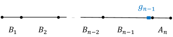
Our main result is built upon three techniques: the subroutine IterativeMinimumBundleKeeping, the subroutine PROP1-PROP, and the Hall matching. The IterativeMinimumBundleKeeping subroutine aims to find a partial allocation that is approximately balanced with most of the goods allocated. It iteratively finds a tentative -partition, finds the bundle with the minimum value by comparison-based queries, and keeps this bundle. This subroutine is the key building block in all our algorithms. By using this subroutine, we can design algorithms for computing PROP1 and EF1 allocations when agents’ valuations are identical.
Roughly speaking, the PROP1-PROP subroutine decides if a bundle approximately meets the proportional requirement of an agent. Specifically, as we will discuss at the beginning of Sect. 3, it is impossible to check with comparison-based queries whether an allocation satisfies the PROP1 condition for an agent or whether a bundle is worth at least of this agent’s value on the entire item set (it is perhaps interesting to see that computing a PROP1 allocation is possible while checking if an allocation is PROP1 is impossible). The PROP1-PROP subroutine takes a bundle and an agent as inputs, and outputs “yes” if the bundle satisfies the PROP1 requirement for the agent, and “no” if the bundle is worth less than of this agent’s value on the entire item set. Notice that a bundle may satisfy both “yes” and “no” conditions; in this case, both outputs “yes” and “no” are acceptable.
With the subroutine PROP1-PROP, given bundles, we can construct a bipartite graph where contains vertices representing the agents, contains vertices representing the bundles, and an edge indicates a bundle surely satisfies the PROP1 requirement for an agent. To find a PROP1 and -MMS allocation, we iteratively find a matching from to such that there is no edge from an agent in to a bundle in , and allocate the bundles in to the agents in . This property guarantees that the agents in believe the remaining unallocated items (the union of the bundles in ) are still worthy enough so that they will receive a bundle satisfying the PROP1 and -MMS conditions in the future. Such matching can be found by removing all the agents in that fail the Hall condition , and we call the matching from to a Hall matching.
The relationship between our techniques and our results is shown in Fig. 1. In Sect. 3, we present an algorithm with queries that finds a PROP1 allocation. In Sect. 4, we discuss our results on EF1 allocations. Finally, in Sect. 5, we present our main result, an algorithm with queries that finds an allocation simultaneously satisfying PROP1 and -MMS. Although our result of PROP1 in Sect. 3 is weaker than our main result in Sect. 5 and the latter is not built upon the former, we discuss the PROP1 algorithm first because it illustrates the application of our three techniques in a clearer and simpler way.
2 Preliminaries
Let denote . There are indivisible goods, denoted by , required to be allocated to agents, denoted by . A bundle is a subset of . An allocation is a -partition of the set of goods , where is the bundle assigned to agent . We say an allocation is a partial allocation if the union of these bundles is a proper set of (i.e., ).
We assume each agent has an intrinsic and non-negative valuation function . The set of all valuation functions is called value profile , and they are not given as input. To learn about an agent’s preference, an algorithm is only allowed to select an agent, present her with two bundles, and ask which one she prefers. Note that even if we could get the comparison result between the two bundles’ utilities, we still do not know the explicit values of the two bundles. We refer to our query model as the comparison-based query model.
Definition 2.1.
In the comparison-based query model, we adopt the following query:
-
•
: given two bundles , let agent compare and , and return the bundle with a higher value (if , she could return an arbitrary one).
Throughout this paper, we assume all the valuation functions are additive, that is, for any and . For simplicity, we refer to as . We say the valuation functions are identical if .
To measure fairness, the most natural notions are envy-freeness (EF) and proportionality (PROP).
Definition 2.2 (EF).
An allocation is said to satisfy envy-freeness (EF) if for any two agents and .
Definition 2.3 (PROP).
An allocation is said to satisfy proportionality (PROP) if for any agent .
However, EF and PROP may not always be satisfied, for example, when . Hence, we consider the following relaxations, EF1 and PROP1. For a verbal description, EF1 says that, for any two agents and , after removing an item from agent ’s bundle, agent will no longer envy agent . PROP1 ensures that, for every agent , there exists an item , such that the total value of agent ’s allocation is at least of the overall value (i.e., ) if that item is included in agent ’s bundle.
Definition 2.4 (EF1).
An allocation is said to satisfy envy-freeness up to one item (EF1) if, for any two agents and , either or there exists an item such that .
Given a (partial) allocation , we say that agent envies agent if .
Definition 2.5 (PROP1).
An allocation is said to satisfy proportionality up to one item (PROP1), if for any agent , there exists an item such that .
To find an EF1 allocation for general monotonic valuation functions, Lipton et al. [26] proposed the tool of envy-graph, where each vertex corresponds to an agent and there is a directed edge from vertex to vertex if agent envies agent . The envy-graph procedure starts from an empty allocation. When there is an unallocated item, it selects a source agent (an agent whose corresponding vertex in the envy-graph has no incoming edges) and assigns that item to her, and then runs the cycle-elimination algorithm until there are no cycles in the envy-graph.
Definition 2.6 (Cycle-elimination).
If there is a cycle on the envy-graph, shift the bundles along this path (i.e., agent receives agent ’s bundle).
In addition to the above two fairness notions, maximin share (MMS) is also an extensively studied fairness notion for indivisible items. The maximin share of agent , denoted by , is defined as the maximum value of the least preferred bundle among all allocations under valuation function . By the definition of MMS, we can observe that . An allocation is said to be MMS-fair if the value of the bundle each agent receives is at least . However, exact MMS-fair allocations may not always exist [31]. An allocation is said to be -maximin share fair (-MMS) if for each agent , she receives a bundle with at least -fractional of her maximin share.
Definition 2.7 (MMS).
Let be the set of all the possible allocations. The maximin share of agent is defined as .
Definition 2.8 (-MMS).
An allocation is said to satisfy -maximin share fair (-MMS), if for any agent , .
In this paper, we mainly study the problem of optimal query complexity (defined as the minimum number of comparison-based queries required) to find a fair allocation. Note that the algorithms in this paper are restricted to deterministic algorithms. We first show a lower bound of the query complexity for finding allocations satisfying the above fairness notions. As illustrated in Section 6, the effect of one comparison-based query can be simply achieved by two valued-based queries. This directly implies that the lower bound of query complexity of the comparison-based query is at least half of the one for the value-based query. In Appendix A.1, we present a counter-example (using similar ideas of the construction in Theorem 5.5 in Oh et al. [27]) indicating the value-based query complexity for PROP1 will be , which directly implies Theorem 2.9.
Theorem 2.9.
The comparison-based query complexity of computing a PROP1/EF1/-MMS allocation is even for a constant number of agents with identical valuations. Here, is an arbitrary real number in .
3 Query Complexity of PROP1
In this section, we focus on the query complexity to find a PROP1 allocation. A straightforward idea is to adapt the moving-knife method [36, 13, 8] or binary search for indivisible items, which intuitively costs about queries. However, under the comparison-based query model, it is impossible to determine whether a bundle is PROP1 (or PROP) for an agent. The following are two counter-examples.
-
•
There are items and agents with identical valuation function when , which is defined as and , where . To determine whether an empty set is PROP1, an algorithm must determine whether , which is equivalent to checking whether . However, this cannot be achieved by the comparison-based query.
-
•
There are three items and three agents with identical valuation function , which is defined as , where . To check whether is PROP, we must figure out whether . However, it is impossible to achieve by the comparison-based query.
To address this issue, we define a subroutine PROP1-PROP-Subroutine in Theorem 3.5, which allows the overlapping of ‘yes’ bundles (satisfying PROP1) and ‘no’ bundles (not satisfying PROP). We show that the subroutine is enough for finding a PROP1 for non-identical additive valuations in Theorem 3.6. In the following, we first consider a special case where the valuations are identical.
Theorem 3.1.
For identical and additive valuation, a PROP1 allocation can be found by Algorithm 1 via queries with running time .
In Algorithm 1, we first execute the ItemPartition subroutine in Algorithm 2. When there are less than items remaining, the update process of ItemPartition may fail: it is possible that and for the bundle with the smallest value. Hence, we begin the second phase (Line 1-1 of Algorithm 1). We first sort the bundles and, without loss of generality, assume . Then in each round, assume there are remaining unallocated items and, without loss of generality. We add the unallocated items to the bundles with the smallest values respectively. If the smallest bundle remains within the bundles, we assign the new item to this bundle, return other new items to the pool, and swap bundles to maintain . Otherwise, if the smallest bundle is no longer among the bundles, we directly assign each item to bundle for each agent and terminate our algorithm.
The correctness of Theorem 3.1 directly follows from Lemma 3.2 and Lemma 3.3 which ensure the fairness and query complexity of the algorithm respectively.
Lemma 3.2.
The allocation returned by Algorithm 1 is PROP1.
Proof.
We assume for simplification and obtain two major observations during Algorithm 2’s execution. First, for each step of the algorithm, for each . Otherwise, consider the while-loop iteration where was updated to its current value : we update where has the smallest value among the bundles in the allocation ; in this case, , which leads to a contradiction. Second, among all the bundles that are updated in the last iteration of the algorithm, denoted by , there exists at least one bundle such that . Otherwise, according to the first observation, .
Next, we claim that our algorithm always executes the ‘if’ branch (Line 1 of Algorithm 1) and terminates after that. Otherwise, there will be only one remaining item in the last round. Since the ‘if’ condition is not satisfied, we have . However, the first observation shows that , hence, , which contradicts to the second observation.
Assume when the ‘if’ branch executes, there are items remaining. Then, according to the second observation, there exists a bundle and an item such that and , hence, . Further, since for and for , we conclude the allocation is PROP1. ∎
Lemma 3.3.
Both the query complexity and running time of Algorithm 1 are .
Proof.
In the first phase, we execute the ItemPartition subroutine with query complexity and running time of as shown in Lemma 3.4. In the second phase, there are less than remaining items, so it runs for at most rounds. In each iteration, we find the maximal bundle and swap bundles to update the sorting, which cost . Hence, both the overall query complexity and running time are . ∎
Lemma 3.4.
Both the query complexity and running time of Algorithm 2 are .
Proof.
Finding the smallest bundle costs queries in each iteration and the size of the unallocated pool roughly decreases by , hence . ∎
Before moving on to additive valuations, we first define PROP1-PROP-Subroutine as mentioned before, which verifies whether or for some item . To do that, an intuitive approach is to adapt Algorithm 1 with queries, where the detailed algorithm and proof are deferred to Appendix B. In Algorithm 3, we implement the subroutine with a lower complexity of (proved in Theorem 3.5).
Specifically, in Algorithm 3, for an agent with valuation function and a bundle , we partition the items into a sequence such that each bundle is weakly more valuable than subject to . Here, some of the items and bundles may be empty because of the lack of items, which will not affect the correctness of our algorithm, and we can directly ignore the corresponding inequalities for these terms. If there are no remaining items in the sequence, i.e., , this implies PROP1 and the algorithm outputs ‘yes’. Otherwise, is not PROP, and the algorithm outputs ‘no’.
Note that the range of ‘yes’ and ‘no’ may overlap. If a bundle is no more than the proportional value but satisfies PROP1, then the algorithm may either output ‘yes’ or ‘no’.
Theorem 3.5.
PROP1-PROP-Subroutine in Algorithm 3 determines if a bundle is PROP1 or not PROP: Given a constant number of agents , a bundle , for a valuation function , is PROP1 if ‘yes’ is returned and is not PROP if ‘no’ is returned via at most queries and the same running time.
Proof.
The query complexity to find each bundle and item is using binary search, hence the overall query complexity and running time of Algorithm 3 is .
For simplification, we assume . If the algorithm outputs ‘yes’, we prove that satisfies PROP1 by contradiction. Let be the most valuable item within . If does not satisfy PROP1, . Then,
which violates . Hence satisfies PROP1.
If the algorithm outputs ‘no’, we have
hence , which indicates does not satisfy PROP. ∎
Based on Theorem 3.1 and PROP1-PROP-Subroutine, we present our following result for additive valuations.
Theorem 3.6.
For non-identical additive valuations, a PROP1 allocation can be found by Algorithm 4 via queries with running time .
Our algorithm works as follows. We first choose an arbitrary agent . Then we follow the Algorithm 1 for the identical case. In particular, we only query agent ’s valuation function . We let the output partition be , where every bundle is PROP1 to agent . A bipartite graph is constructed where the two sets of vertices are, respectively, the agents and the bundles in . The edges in the graph are constructed through PROP1-PROP-Subroutine, where if agent says ‘yes’ to bundle , we add an undirected edge , and we further add edges between agent and each bundle. We can observe that an agent will not answer ‘no’ to all bundles since the value of each bundle cannot be less than at the same time. Hence, the number of created edges will be non-zero. Then, we find a maximal subset of the agents such that its size is larger than its neighbors’ size greedily. Denote this maximal subset by and the neighbors of by , and the complementary of these two sets by and respectively. As agent is adjacent to all bundles from Line 4, , thus . A perfect matching can be found between and a subset of as shown in Lemma 3.7, where each agent in is matched to an adjacent bundle and some bundles in may remain unmatched, and each matched bundle is allocated to the matched agent. For the remaining agents in and the unallocated items in , we repeat the above process with a decreased number of agents and items until each agent receives a bundle.
Similarly, Lemma 3.8 and Lemma 3.9 indicate the correctness of Theorem 3.6. We first show our algorithm works correctly in Lemma 3.7.
Proof.
We show the induced subgraph containing , , and the edges between them satisfy Hall’s marriage theorem.111Hall’s marriage theorem says that: for a bipartite graph , if for any subset , we have , then there exists a perfect matching which can match each vertex in to an adjacent vertex in . [23] Each vertex is adjacent to at least one vertex in and for each subset , . Otherwise, in both cases, we may add or to to obtain a larger , which contradicts that is maximal. Hence, a perfect matching can always be found between and a subset of . ∎
Lemma 3.8.
The allocation returned by Algorithm 4 is PROP1.
Proof.
First, each agent will receive a bundle through our algorithm. In each iteration of the ‘while’ loop, the matched agents in set can receive a bundle as Lemma 3.7. Further, from , at least one agent is matched to a bundle in the iteration.
Second, we show each agent’s bundle is PROP1 by induction. For each agent in that receives a bundle from the matching in the first iteration, she thinks the bundle is PROP1 as PROP1-PROP-Subroutine outputs ‘yes’. For each agent in that does not receive any bundle, she thinks the value of each matched bundle in is less than her proportional value among the whole item set, otherwise, the subroutine will output ‘yes’ and the bundle will belong to , hence, cannot be matched. We then consider an agent who is matched in the -th iteration (). Denote by the number of all the unmatched agents before the -th iteration and the total value of all the unallocated items before the -th iteration under valuation function . Similar to the above analysis, agent receives a PROP1 bundle with respect to and , and she thinks the bundles allocated in -th iteration is less than . This leads to,
which indicates also satisfies PROP1 to agent in the -th iteration. Repeating this process, we can conclude , hence, the lemma holds. ∎
Lemma 3.9.
Both the query complexity and running time of Algorithm 4 are .
Proof.
As we have shown, the running time for computing a PROP1 allocation at Line 4 is , and constructing a bipartite graph invokes PROP1-PROP-Subroutine times between each agent and each bundle at Line 4. Finding the maximal subset costs and if , finding the perfect matching costs by the Hungarian algorithm, and both of them invoke no query. Hence, we may write the running time of Algorithm 4 as
In the worst case, , hence .
The query complexity can be obtained by
∎
4 Query Complexity of EF1
This section studies the query complexity to compute an EF1 allocation. For a constant number of agents, the well-known Round-Robin algorithm that guarantees EF1 requires queries as each agent needs to sort the items in descending order, and the envy-graph procedure requires queries as each round of the procedure allocates one item and costs a constant number of queries. There is still a gap between the existing algorithms and the lower bound of computing an EF1 allocation under the comparison-based query model for a constant number of agents. In this section, we endeavor to bridge this gap and improve the query complexity for computing an EF1 allocation.
Theorem 4.1.
For two agents with additive valuations, the query complexity and running time of computing an EF1 allocation are .
Proof.
For two agents, a straightforward algorithm cut-and-choose can output an EF1 allocation. In the cut-and-choose algorithm, the first agent divides all the items into two bundles, where she perceives the allocation as EF1 regardless of which bundle she receives. Then, the second agent chooses a bundle that she feels is more valuable. We can easily verify that the allocation is EF1 to the first agent and envy-free to the second agent. The query complexity mainly depends on the first agent’s division step, as the second agent’s choosing step only requires one query.
For the division step, we claim it can be achieved in queries by adopting the binary search method. We arrange all the items in a line. For any given item , we define the bundle to the left of as ( is not included in ), and the bundle to the right of as ( is not included in ). Our goal is to find the rightmost item such that . It is straightforward that such an item exists due to the interpolation theorem, and can be found through a binary search algorithm. Then a valid partition for the first agent is .
Therefore, the overall query complexity and running time are . ∎
We now come to our main result in this section that for identical valuation, the query complexity for EF1 is , which provides a tight query complexity for a constant number of agents.
Theorem 4.2.
For identical and additive valuations, an EF1 allocation can be found via queries with running time .
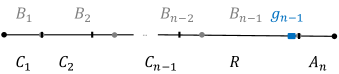
The case of is trivial. Here we focus on the case of . Our algorithm works as follows and is illustrated in Fig. 2.
Step 1: We run the subroutine ItemPartition() in Algorithm 2. The algorithm returns a partial allocation and a set of unallocated items .222We can verify that there will always be exactly unallocated items when Algorithm 2 terminates. Consider the last round. Either two items will be allocated from a set of items, or one item will be allocated from a set of exactly items. In both cases, there will be exactly items remaining. Without loss of generality, assume and .
Step 2: We go back to the round in which was last updated in Algorithm 2. In that round, we have a temporary allocation such that is the one with the smallest utility among all. We only focus on and assume the bundle containing is (if not, we switch it with ). We line up the bundles from the left to the right in the order of and, in particular, arrange in the right of such that is adjacent to .
Step 3: Update the first bundles in a moving-knife manner. We find another bundles from left to right such that each for is weakly larger than and smaller than after removing ’s rightmost item, which ensures the EF1 conditions from to and from to . As is not larger than with , the right endpoint of bundle is to the left of (or at most the same as) , which means such an allocation (maybe partial) exists. If there is no unallocated item between and , an EF1 allocation is already found.
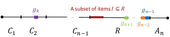
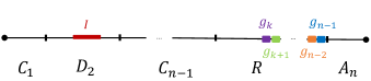
Step 4: If there are still unallocated items, denote them by . We have as it is placed directly to the left of . If is the only item in , we proceed to Step 5.
Otherwise, we proceed with the following operations in the order of , , , and exchange each of them with items of . For clarity, as shown in Fig. 2(c), if the bundle contains , is exchanged to in Fig. 2(d), while some items from are exchanged to so that the new bundle is still weakly larger than or equal to (to guarantee EF). We refer to the new bundle after exchange as for each . Note that the unallocated items are also arranged in a line. During each exchanging operation, the items in are taken from the leftmost end, and the returned item is arranged such that the rightmost items are for some . Repeat this process until no more exchange can be made or . Then, we obtain a partial allocation and a set of unallocated items .
Step 5: Allocate to an arbitrary agent. For the remaining items in , run the envy-graph procedure to allocate them based on the partial allocation .
Lemma 4.3.
The allocation returned by the above procedure is EF1.
Proof.
First, as we have guaranteed in our algorithm, for each bundle in after Step 3, is EF1 to and is EF to . Then, for any two bundles and , there exists an item such that . Hence, the (partial) allocation satisfies EF1.
If a complete allocation has not been found, our algorithm proceeds to Step 4. In Step 4, as we still ensure is EF1 to each updated bundle , we can show that also satisfies EF1 using a similar analysis as above.
Finally, in Step 5, as we will show in Lemma 4.4, the utility of will always be zero, which does not destroy EF1. In addition, since the envy-graph procedure maintains the property of EF1, we eventually obtain a complete EF1 allocation. ∎
To show our algorithm runs in query complexity, we need to guarantee that the number of items that are allocated through the envy-graph procedure in Step 5 is not too large. Lemma 4.4 claims that the number of the unallocated items in after Step 4 is at most .
Lemma 4.4.
After Step 4, or .
Proof.
For simplification, we assume . As we have shown in the proof of Lemma 3.2, for each , we have . Assume , since , we have
We show that if , then . Denote in each iteration by . Assume that we have already completed the exchange from to , then the order of items in is . Now we are about to exchange with some items in and assume is in the bundle .
The exchange step can be divided into three cases:
-
•
If , then the algorithm terminates with for . The order of is still .
-
•
If is already weakly larger than after receiving only a subset of , i.e., there exists a subset and an item , such that and , we exchange with . The order of will be updated to .
-
•
Otherwise, we have . Then, we exchange with and terminates the algorithm. Specifically, is EF1 to since . As , we also have . The order of will be updated to .
The only case when is that our algorithm terminates after the aforementioned second case and there are still items remaining in , which means contains all the items from to and . However, if , as for , it leads to
which contradicts to the assumption . Hence, we conclude that or . ∎
Lemma 4.5.
Both the query complexity and running time of the above procedure are .
Proof.
In Step 1, the subroutine ItemPartition requires queries as analyzed in Lemma 3.3. In Step 3, as the items are arranged in a line, the moving-knife method for each bundle can be implemented using binary search to find the rightmost end of the bundle , costing queries in total. Similarly, the exchange operation for each bundle in Step 4 can also be done via binary search in queries. Finally, as we have shown in Lemma 4.4, after Step 4, or . That means there are at most remaining items to be allocated during the envy-graph procedure. Constructing the envy-graph for the first time costs queries to sort the bundles. Then, in each iteration, after an item is allocated to the smallest bundle, we only need to sort this specific bundle based on the original order, which can be done using queries via binary search. Hence, we conclude that both the query complexity and running time are . ∎
We further consider the query complexity for three agents with additive valuations. This algorithm is almost a straightforward adaption of Algorithm 3 of [27], where the algorithm for identical valuation in Theorem 4.2 is adapted. The detailed algorithm and its proof are deferred to Appendix C.1.
Theorem 4.6.
For three agents with additive valuations, the query complexity and running time of computing an EF1 allocation are .
5 Query Complexity of MMS+PROP1
For a constant number of agents with additive valuations, we have already shown that a PROP1 allocation can be found via queries. Besides PROP1, MMS is also a well-studied fairness notion in the fair division of indivisible goods. In this section, we will provide an algorithm that can achieve PROP1 and -MMS simultaneously via queries, which is shown in Algorithm 5.
Before the detailed descriptions of our algorithm, we first define two types of bundles given by our algorithm. We call the bundle in Line 5 and the bundle in Line 5 bundles of the first type and the bundle in Line 5 bundles of the second type.
Similar to Algorithm 4, we perform a multi-round algorithm. For each round, according to the set of agents not receiving any items and the set of unallocated items, we first choose an arbitrary agent and find a PROP1 and -MMS allocation subject to agent ’s valuation , corresponding to Lines 5-5 in Algorithm 5. In this part, we first use the subroutine ItemPartition defined in Algorithm 2 to find the partial allocation and a set of unallocated items whose size is less than . Lines 5-5 corresponds to the first case where the two most valuable bundles among all bundles in and all items in are both items in . In this case, we can directly allocate the most valuable item in to agent and restart the main procedure for the remaining items and agents by ignoring all previous bundles of the second type. Otherwise, we can run the procedure described in Theorem 4.2 to obtain an EF1 allocation under , which is the wanted PROP1 and -MMS allocation under valuation .
We then perform Lines 5-5 to construct a bipartite graph between all remaining agents in and all bundles in the above EF1 allocation , similar to the BipartiteConstruction function in Algorithm 4. Here, an edge between an agent and a bundle is constructed only if allocating to agent can meet agent ’s requirement for both PROP1 and -MMS. We first execute the PROP1-PROP-Subroutine in Algorithm 3 to identify the bundles that satisfy PROP1 to agent . However, different from that used in Algorithm 4, we also need to ensure -MMS here. Thus, we consider the allocation in two subcases. Lines 5-5 perform the first case where agent can receive only one item in to reach both PROP1 and -MMS. Under this case, we can again allocate the most valuable item to agent and restart the main procedure with only the bundles of the first type allocated. Otherwise, we can claim that agent can meet the requirement for PROP1 and -MMS after receiving , corresponding to Line 5 of Algorithm 5.
Lines 5-5 perform a similar reduction procedure as used in Algorithm 4, where we find a maximal subset that violates Hall’s marriage theorem. We then find a perfect matching of the remaining agents to some bundles and reduce the original instance to a smaller instance after removing these agents and their matched bundles.
We now can present our main theorem in this section.
Theorem 5.1.
For additive valuations, a PROP1 and -MMS allocation can be found by Algorithm 5 via queries with running time .
We first use the following lemma to show that removing the bundles of the first type directly will not damage the PROP1 and MMS conditions.
Lemma 5.2.
For an instance which allocates a set of indivisible goods to a set of agents, fixing an agent and a good , we can define and for each agent as the maximum share of agent under the original instance and the instance removing agent and the good from . We also assume a PROP1 allocation for . For each , we have:
-
•
;
-
•
there exists an item such that .
Proof.
We fix an agent . We assume of is obtained from an allocation . Since the only difference between instances and is the agent and the good , removing the good in and reallocating the other items in the bundle containing to other bundles can lead to an allocation in with a weakly larger maximin share. Thus, .
For the second part, if , holds directly. Otherwise, we have , so . Since is PROP1 in instance , by definition, there exists an item such that . ∎
Since the bundles of the first type only contain exactly one item, if the allocation containing only the bundles of the second type is PROP1 and -MMS under the reduced instance, by Lemma 5.2, these bundles can also meet the conditions of PROP1 and -MMS under the original instance. Thus, we will first assume there is no bundle of the first type and check the properties for the bundles of the second type in the following.
Before we start our proof, we first present two lemmas which will be proved later.
Lemma 5.3.
For the set of unallocated items and the set of agents not receiving items during the procedure, for any and any , we have .
Lemma 5.4.
For the set of unallocated items and the set of agents not receiving items during the procedure, for any , we have .
These two lemmas can help us to keep the PROP1 and MMS properties during the reduction of the problem.
Lemma 5.5.
The allocation output in Line 5 is PROP1 and the valuation of each bundle is at least under for the instance which allocates the set of items to the set of agents.
Proof.
From the procedure described in Theorem 4.2, the allocation is an EF1 allocation under and for each , where is defined in Line 5 of Algorithm 5. Consider the partial allocation and the unallocated items output by ItemPartition under the valuation , since the condition at Line 5 is not met, is one of the two largest values among the values of each bundle in and each item in . If is the largest one, we have from and Lemma 5.4. If is the second largest one, the largest one should be a single item, by Lemmas 5.2 and 5.3, removing this item and one arbitrary agent, we have . Thus, is -MMS under .
For PROP1, since is an EF1 allocation under , this implies PROP1. ∎
From Lemma 5.5, we get the correctness of the edges added in Line 5. We next show all added edges in Line 5 also satisfy the corresponding conditions for PROP1 and -MMS.
Lemma 5.6.
For each added edge in Line 5, allocating to agent can meet the conditions for PROP1 and under the instance that allocates the set of items to the set of agents.
Proof.
The PROP1 condition is satisfied for the same reason as in Theorem 3.5. For the -MMS condition, since the condition in Line 5 is not met, must be one of the two largest among under . From the same analysis as in the proof of Lemma 5.5, the -MMS condition for agent receiving the bundle is satisfied. ∎
From the previous two lemmas, we can conclude that the bundles of the second type in Line 5 can satisfy the PROP1 and -MMS conditions under the corresponding instance of items and agents . From the existence of the set and the perfect matching in Lines 5-5 which can be shown in the same way as in Lemma 3.7, it suffices to show: the feasibility of the PROP1 conditions under the reduced instance can induce the feasibility of the PROP1 conditions in the original instance and Lemma 5.3 holds.
For the induction of the PROP1 conditions, this can be directly reached from the correctness of Lemma 5.4. According to Theorem 3.5, in any round which allocates a set of unallocated items to a set of agents, each matched in this round is valued less than under the valuation for each . From this, we can observe that the term for each remaining agent becomes larger after this round. Summarizing over all rounds, we can conclude the statement in Lemma 5.4.
We then show Lemma 5.3 holds. To show this lemma, it suffices to show the following lemma.
Lemma 5.7.
In any round which allocates a set of items to a set of agents, for each remaining agent , we can partition the set of the remaining items into bundles such that values each bundle weakly larger than those allocated bundles in this round in Line 5.
If the previous lemma holds, for any and any mentioned in the statement of Lemma 5.3, we can remove the corresponding bundle containing in agent ’s partition in the previous round from Lemma 5.7 and put the items except in this bundle to an arbitrary bundle. From the fact that values each bundle weakly larger than those allocated bundles in this round, we have , where and are the corresponding sets in the previous round. By recursion over the rounds, we can finally get Lemma 5.3.
Proof of Lemma 5.7.
Fix an agent and we assume that the allocated bundles in this round are where . Here, . We find the corresponding for agent and the bundle . We then can treat each as one of the initial bundles where each one has the weakly larger utility than under . We then consider . Since and all items in must be placed continuously by the rearrangement at Line 5 after treating the sequence as a cycle, can intersect at most of . We then can remove and merge the two sets which contain some elements in . From , the merged bundle still has a weakly larger utility than under . If is contained in exactly one set, we can directly remove that set. We then take similar steps for the remaining and conclude our lemma. ∎
We have already shown the bundles of the second type satisfy the conditions for PROP1 and -MMS above, it suffices to show they also hold for the bundles of the first type to prove the correctness of our algorithm.
Lemma 5.8.
For a bundle of the first type allocated to an agent , and there exists a good such that .
Proof.
We finally consider the query complexity of our algorithm.
Lemma 5.9.
Both the query complexity and running time of Algorithm 5 are .
Proof.
In each iteration, the size of is decreased by at least . We consider the query complexity and running time within each iteration.
At Lines 5-5, the ItemPartition Subroutine is invoked for an agent and she is asked to find the two most valuable bundles, costing queries. In Line 5, both the query complexity and running time to construct an EF1 allocation under is . We then consider the second part, corresponding to Lines 5-5. By using the binary search technique in Line 5, it costs queries for each agent to construct the bundles from each and to find the two most valuable bundles in Line 5. Finally, finding the maximal subset in Line 5 costs and if , finding the perfect matching costs in Line 5, and both of them invoke no query.
Then, in the worst case, the running time is
hence, .
Similarly, the query complexity is
∎
6 Related Work
There have been several studies on value-based query complexity for computing fair allocations of indivisible items [28, 27]. This type of value-based query allows the algorithm to select a bundle and an agent and acquire agent ’s specific value for that bundle of items (i.e., ). Observe that each comparison-based query can be simulated by two value-based queries, which implies that the lower bound of comparison-based query complexity is no less than the one of value-based query complexity asymptotically. For value-based queries, Plaut and Roughgarden [28] showed that, even for two agents with identical and monotone valuations, the query complexity of computing an EFX (envy-free up to any item, a stronger notion than EF1) allocation is exponential in terms of the number of indivisible items. Their proof is based on a reduction from the local search problem of the Kneser graph. Note also that the query complexity of computing an EFX allocation for identical and additive valuations is . Furthermore, Oh et al. [27] explored the value-based query complexity for more fairness notions. They mainly considered the case of monotone valuations. For the EFX criterion, for two agents, they gave a lower bound of queries and a matching upper bound of queries for additive valuations. For the EF1 criterion, with no more than three agents, they found the query complexity is exactly for additive valuations. They also provided an algorithm using queries for three agents with monotone valuations. With more than three agents, they provided a careful analysis of the complexity of the classic envy-graph procedure, which requires queries in the worst case.
In the context of fair division of divisible resources (i.e., the cake-cutting problem), a valuation function in the cake-cutting problem can be a general real function on an interval, which makes it impossible to be succinctly encoded. Thus, the query complexity has been extensively studied in the cake-cutting problem [9, 33, 37, 25, 3, 4, 32, 11, 15]. The most well-known query model is the Robertson-Webb (RW) query model [33], where two types of queries, namely Eval and Cut, are allowed. In particular, asks agent the value of interval and asks agent to report a point such that , where denote agent ’s value of interval . For finding a proportional allocation, the moving-knife algorithm [18] and the Even-Paz algorithm [20] could compute a proportional allocation with connected pieces within the complexity of and RW queries, respectively. On the other hand, Edmonds and Pruhs [19] gave a lower bound of RW queries. Computing an envy-free allocation is more challenging. For two agents, an envy-free allocation can be simply found by the cut-and-choose protocol. For a general number of agents, Aziz and Mackenzie [4] proposed an algorithm for computing an envy-free allocation within a finite number of RW queries while the best known lower bound is due to Procaccia [30].
However, all the query models mentioned above require agents to answer the query with numbers that typically represent values for subsets of the resources. To the best of our knowledge, we are the first to consider the comparison-based query model in fair division.
Another related type of complexity model in fair division is the communication complexity in which the amount of communication that the agents need to exchange (between themselves or with a mediator) is computed [29, 10]. Our problem is also implicitly related to fair division of indivisible goods using only ordinal or partial information about the preferences (e.g., [24, 6, 7]), we refer to the excellent survey for an overview of recent progress on fair allocations of indivisible goods [2].
7 Conclusion and Future Work
In this work, we proposed the comparison-based query model, where the valuation functions are not provided as the input to the allocation algorithms. Our model provides a new approach to access the agents’ preferences for items. A highlight of our algorithms is that our results just rely on the comparison result between bundles, rather than the concrete values. Moreover, we also studied the query complexity of computing a fair allocation and provided an efficient algorithm to compute an allocation satisfying both PROP1 and -MMS through at most queries for a constant number of agents. We believe this will provide inspiration for designing algorithms based on comparative relationships.
One of our future directions is to continue the research under the EF1 notion for a constant number of agents and additive valuations. Another interesting future direction is to consider general valuation functions (e.g., submodular valuations and monotone valuations) beyond additive ones.
References
- Akrami and Garg [2024] Hannaneh Akrami and Jugal Garg. Breaking the barrier for approximate maximin share. In Proceedings of the ACM-SIAM Symposium on Discrete Algorithms (SODA), pages 74–91, 2024.
- Amanatidis et al. [2023] Georgios Amanatidis, Haris Aziz, Georgios Birmpas, Aris Filos-Ratsikas, Bo Li, Hervé Moulin, Alexandros A. Voudouris, and Xiaowei Wu. Fair division of indivisible goods: Recent progress and open questions. Artificial Intelligence, 322:103965, 2023.
- Aziz and Mackenzie [2016a] Haris Aziz and Simon Mackenzie. A discrete and bounded envy-free cake cutting protocol for four agents. In Proceedings of the Annual ACM Symposium on Theory of Computing (STOC), pages 454–464, 2016a.
- Aziz and Mackenzie [2016b] Haris Aziz and Simon Mackenzie. A discrete and bounded envy-free cake cutting protocol for any number of agents. In Proceedings of the Annual IEEE Symposium on Foundations of Computer Science (FOCS), pages 416–427, 2016b.
- Aziz et al. [2022] Haris Aziz, Ioannis Caragiannis, Ayumi Igarashi, and Toby Walsh. Fair allocation of indivisible goods and chores. Autonomous Agents and Multi-Agent Systems, 36(1):3:1–3:21, 2022.
- Aziz et al. [2023] Haris Aziz, Bo Li, Shiji Xing, and Yu Zhou. Possible fairness for allocating indivisible resources. In Proceedings of the International Conference on Autonomous Agents and Multiagent Systems (AAMAS), pages 197–205, 2023.
- Benadè et al. [2022] Gerdus Benadè, Daniel Halpern, and Alexandros Psomas. Dynamic fair division with partial information. In Proceedings of the Annual Conference on Neural Information Processing Systems (NeurIPS), pages 3703–3715, 2022.
- Bilò et al. [2022] Vittorio Bilò, Ioannis Caragiannis, Michele Flammini, Ayumi Igarashi, Gianpiero Monaco, Dominik Peters, Cosimo Vinci, and William S. Zwicker. Almost envy-free allocations with connected bundles. Games and Economic Behavior, 131:197–221, 2022.
- Brams and Taylor [1995] Steven J Brams and Alan D Taylor. An envy-free cake division protocol. The American Mathematical Monthly, 102(1):9–18, 1995.
- Brânzei and Nisan [2019] Simina Brânzei and Noam Nisan. Communication complexity of cake cutting. In Proceedings of the ACM Conference on Economics and Computation (EC), page 525, 2019.
- Brânzei and Nisan [2022] Simina Brânzei and Noam Nisan. The query complexity of cake cutting. In Proceedings of the Annual Conference on Neural Information Processing Systems (NeurIPS), pages 37905–37919, 2022.
- Bu et al. [2022] Xiaolin Bu, Zihao Li, Shengxin Liu, Jiaxin Song, and Biaoshuai Tao. On the complexity of maximizing social welfare within fair allocations of indivisible goods. arXiv preprint arXiv:2205.14296, 2022.
- Budish [2011] Eric Budish. The combinatorial assignment problem: Approximate competitive equilibrium from equal incomes. Journal of Political Economy, 119(6):1061–1103, 2011.
- Caragiannis et al. [2019] Ioannis Caragiannis, David Kurokawa, Hervé Moulin, Ariel D Procaccia, Nisarg Shah, and Junxing Wang. The unreasonable fairness of maximum Nash welfare. ACM Transactions on Economics and Computation (TEAC), 7(3):1–32, 2019.
- Cechlárová and Pillárová [2012] Katarína Cechlárová and Eva Pillárová. On the computability of equitable divisions. Discrete Optimization, 9(4):249–257, 2012.
- Chaudhury et al. [2023] Bhaskar Ray Chaudhury, Jugal Garg, and Kurt Mehlhorn. EFX exists for three agents. Journal of the ACM (JACM), 2023. Forthcoming.
- Conitzer et al. [2017] Vincent Conitzer, Rupert Freeman, and Nisarg Shah. Fair public decision making. In Proceedings of the ACM Conference on Economics and Computation (EC), pages 629–646, 2017.
- Dubins and Spanier [1961] Lester E Dubins and Edwin H Spanier. How to cut a cake fairly. The American Mathematical Monthly, 68(1P1):1–17, 1961.
- Edmonds and Pruhs [2006] Jeff Edmonds and Kirk Pruhs. Cake cutting really is not a piece of cake. In Proceedings of the ACM-SIAM Symposium on Discrete Algorithms (SODA), pages 271–278, 2006.
- Even and Paz [1984] Shimon Even and Azaria Paz. A note on cake cutting. Discrete Applied Mathematics, 7(3):285–296, 1984.
- Foley [1967] Duncan Karl Foley. Resource allocation and the public sector. Yale Economics Essays, 7(1):45–98, 1967.
- Ghodsi et al. [2021] Mohammad Ghodsi, Mohammad Taghi Hajiaghayi, Masoud Seddighin, Saeed Seddighin, and Hadi Yami. Fair allocation of indivisible goods: Improvement. Mathematics of Operations Research, 46(3):1038–1053, 2021.
- Hall [1987] Philip Hall. On representatives of subsets. Classic Papers in Combinatorics, pages 58–62, 1987.
- Halpern and Shah [2021] Daniel Halpern and Nisarg Shah. Fair and efficient resource allocation with partial information. In Proceedings of the International Joint Conference on Artificial Intelligence (IJCAI), pages 224–230, 2021.
- Kurokawa et al. [2013] David Kurokawa, John Lai, and Ariel Procaccia. How to cut a cake before the party ends. In Proceedings of the AAAI Conference on Artificial Intelligence (AAAI), pages 555–561, 2013.
- Lipton et al. [2004] Richard J Lipton, Evangelos Markakis, Elchanan Mossel, and Amin Saberi. On approximately fair allocations of indivisible goods. In Proceedings of the ACM Conference on Electronic Commerce (EC), pages 125–131, 2004.
- Oh et al. [2021] Hoon Oh, Ariel D. Procaccia, and Warut Suksompong. Fairly allocating many goods with few queries. SIAM Journal on Discrete Mathematics, 35(2):788–813, 2021.
- Plaut and Roughgarden [2020a] Benjamin Plaut and Tim Roughgarden. Almost envy-freeness with general valuations. SIAM Journal on Discrete Mathematics, 34(2):1039–1068, 2020a.
- Plaut and Roughgarden [2020b] Benjamin Plaut and Tim Roughgarden. Communication complexity of discrete fair division. SIAM Journal on Computing, 49(1):206–243, 2020b.
- Procaccia [2009] Ariel D Procaccia. Thou shalt covet thy neighbor’s cake. In Proceedings of International Joint Conference on Artificial Intelligence (IJCAI), pages 239–244, 2009.
- Procaccia and Wang [2014] Ariel D Procaccia and Junxing Wang. Fair enough: Guaranteeing approximate maximin shares. In Proceedings of the ACM conference on Economics and computation (EC), pages 675–692, 2014.
- Procaccia and Wang [2017] Ariel D Procaccia and Junxing Wang. A lower bound for equitable cake cutting. In Proceedings of the ACM Conference on Economics and Computation (EC), pages 479–495, 2017.
- Robertson and Webb [1998] Jack Robertson and William Webb. Cake-Cutting Algorithms: Be Fair If You Can. Peters/CRC Press, 1998.
- Steinhaus [1948] Hugo Steinhaus. The problem of fair division. Econometrica, 16(1):101–104, 1948.
- Steinhaus [1949] Hugo Steinhaus. Sur la division pragmatique. Econometrica, 17:315–319, 1949.
- Stromquist [1980] Walter Stromquist. How to cut a cake fairly. The American Mathematical Monthly, 87(8):640–644, 1980.
- Stromquist [2008] Walter Stromquist. Envy-free cake divisions cannot be found by finite protocols. Electronic Journal of Combinatorics, 15(1):#R11, 2008.
- Varian [1974] Hal R Varian. Equity, envy, and efficiency. Journal of Economic Theory, 9(1):63–91, 1974.
Appendix A Omitted Proof of Lower Bound
A.1 Proof of Theorem 2.9
We prove a stronger lower bound for value-based query complexity, which directly implies the lower bound of comparison-based query complexity.
Theorem A.1.
The value-based query complexity of computing a PROP1/EF1/-MMS allocation is for a constant number of agents even with identical valuations. Here, is an arbitrary real number in
Proof.
There are agents with identical and binary valuation functions. Among the items, there are items such that each agent has a value of for each of them and for the remaining items. In this scenario, if an allocation satisfies PROP1 or -MMS for any , each bundle in the allocation should include at least one valued item and, at most, two valued items.
Initially, let be the whole set of items. Then we answer the query in an adversary manner as follows: if , answer and replace by ; else answer and replace by . At each step, the only information the allocator knows is that all the valued items are located in . When , any allocation would contain a bundle with at least three items from . Hence, the algorithm cannot guarantee that every bundle does not contain more than two items of . Thus, the algorithm must keep querying until . Thus, the total query complexity is at least .
As EF1 is a stronger notion than PROP1, the same lower bound for finding an EF1 allocation is directly derived. ∎
Appendix B An Alternative Approach to Defining PROP1-PROP-Subroutine
The primary algorithm for the subroutine is presented in Algorithm 6. Specifically, we first execute Algorithm 1 where we initialize the input number of the agents to be and the input item set to be . The algorithm returns a PROP1 allocation with bundles, and we find the smallest bundle in the allocation, say . We output ‘yes’ if and ‘no’ if .
Correctness of Algorithm 6. Both the query complexity and running time of Algorithm 3 are , the same as in Lemma 3.3.
For simplification, we assume , and . According to Theorem 3.1, is PROP1 for and agents, hence, there exists an item such that . If the algorithm outputs ‘yes’, , then
Hence, bundle satisfies PROP1. If the algorithm outputs ‘no’, then . is not PROP in this case, otherwise, , which contradicts to . ∎
Appendix C Omitted Proof of Query Complexity of EF1
C.1 Proof of Theorem 4.6
Our algorithm works in the following steps:
Step 1: Compute an EF1 allocation with identical valuation function according to the algorithm described in Theorem 4.2. If agent and agent favorite different bundles, then assign the remaining bundle to agent . The current allocation is clearly EF1. Otherwise, without loss of generality, we assume and .
Step 2: Next we arrange items of on a line and use binary search to divide bundle into and such that and , where is the leftmost item of .
-
•
If , then we allocate to agent , to agent and to agent . For item set and identical valuation function , we could compute an EF1 allocation . Then we let the three agents select their preferred bundle in order .
-
•
Otherwise, if , we proceed to the next step.
Step 3: We call an item large if and . Then we will find three large items (if exist) as follows:
First, since obviously satisfies the definition of a large item, it is the first one.
Next, we use binary search to find a set such that and , where is the rightmost item of set .
-
•
If such set and item exist, then remove the items of from and add them to . Thus, is a new large good. If , then we return to step 2 with the updated bundle . Otherwise, the condition still holds. We could continue the above operation until we find three large items.
-
•
Otherwise, if and do not exist, we remove all items except the (up to two) large items from and add them to .
Step 4: Let be agent ’s favourite bundle between and , and let be the other bundle. Then assign to agent and to agent and to agent 1.
Step 5: Compute an EF1 allocation with identical valuation function according to the algorithm in Theorem 4.2, where the three large items are excluded from the item set. Denote the three large items by , and without loss of generality, assume , . Then we obtain an allocation and denote it by .
Step 6: Consider the following cases of the locations of the large items:
-
•
If there exists a large item in each of , , and , then let the three agents take their favorite bundle according to the order .
-
•
Otherwise, that means there are at most two items within . We assign the first large item to agent and the second one to agent .
Proof of Theorem 4.6.
To prove the allocation is EF1, we only need to show after Step 5 is EF1 under the identical valuation function , and the proof in the rest of the part is the same as in [27]. As satisfies EF1, we know for any , there exists an item such that . If , . If , . Hence we conclude satisfies EF1.
As the number of agents is constant, the binary search in Step 2 and Step 3 requires queries. The query complexity to find an EF1 allocation under identical valuation is also according to Lemma 4.5. The other operations in the above algorithm cost queries. Hence, the query complexity of computing an EF1 allocation for three agents is . ∎