Lifshitz transitions and Weyl semimetals
from a topological superconductor with supercurrent flow
Abstract
A current flowing through a superconductor induces a spatial modulation in its superconducting order parameter, characterized by a wavevector related to the total momentum of a Cooper pair. Here we investigate this phenomenon in a -wave topological superconductor, described by a one-dimensional Kitaev model. We demonstrate that, by treating as an extra synthetic dimension, the current carrying non-equilibrium steady state can be mapped into the ground state of a half-filled two-dimensional Weyl semimetal, whose Fermi surface exhibits Lifshitz transitions when varying the model parameters. Specifically, the transition from Type-I to Type-II Weyl phases corresponds to the emergence of a gapless -wave superconductor, where Cooper pairs coexist with unpaired electrons and holes. Such transition is signaled by the appearance of a sharp cusp in the -dependence of the supercurrent, at a critical value that is robust to variations of the chemical potential . We determine the maximal current that the system can sustain in the topological phase, and discuss possible implementations.
I Introduction.
Weyl semimetals (WSMs) and Topological superconductors (TSs) might lead to an actual breakthrough in quantum science and technology.
Indeed WSMs are quite promising for applications in ultra-fast electronics and photonics due to their peculiar linear band spectrum and large carrier mobility [1, 2]. These materials are commonly divided into two families, dubbed Type-I [3, 4] and Type-II [5, 6, 7, 8], depending on the tilting of the cone characterizing their electronic spectrum near special point nodes. In turn, these bulk nodes also protect the existence of topological Fermi arc states on the WSM surfaces [9, 10, 11], as confirmed by various ARPES experiments [12, 13, 14, 15]. While three-dimensional WSMs have been vastly studied, more recently a growing interest is devoted to two-dimensional WSMs, [16, 17, 18, 19, 20], also in view of their possible realization with cold atoms[18].
Similarly, TSs are materials with a huge potential in applications, as they combine two remarkable properties. On the one hand, they host edge modes, known as Majorana quasi-particle (MQPs) [21, 22, 23, 24, 25], featuring peculiar non-local correlations and unconventional braiding properties that could be harnessed for topologically protected quantum computation. On the other hand, they exhibit a dissipationless transport that is ideal to develop green nanoelectronics. Various implementations of TSs, based e.g. on proximized spin-orbit nanowires[26, 27], quantum spin Hall edge systems contacted to ferromagnets[28, 29] and ferromagnetic atom chains[30, 31, 32, 33, 34], have been proposed and are supported by promising, although not yet conclusive, experimental confirmations.[35, 36, 37, 38, 39, 40, 41, 42]
In this work, we show that the phase modulation emerging in the order parameter of a superconductor in the presence of a current flow[43] naturally provides an intriguing connection between TSs and WSMs. Indeed, by treating as an additional synthetic dimension, we show that the nonequilibrium stationary state of the 1D superconductor with a current flow can be mapped onto the ground state of a 2D half-filled fermionic model. As a consequence, the appearance of the various phases of the 1D superconductor can be understood as the result of a Lifshitz transition[44, 45] in the Fermi surface of the associated 2D model. In particular, a 1D -wave TS is mapped onto a 2D WSM[46, 47, 18, 48, 49, 50]. By varying the model parameters, the transition from type-I to Type-II WSM corresponds to the appearance of a gapless superconducting phase in the TS, where Cooper pairs coexist with unpaired electrons and holes. In turn, this also determines a change in the range of -values where the gapped TS exists, which is controlled by its chemical potential or superconducting order parameter, depending on whether the associated WSM is in the Type-I or in the Type-II phase. By exploiting the mapping, we construct the low energy expression of a Fermi “arc” in the 2D WSM and of the Majorana edge mode in the corresponding current-biased 1D superconductor. By contrast, a 1D -wave superconductor corresponds to a 2D insulator or to a 2D conventional semimetal, depending on the parameter range. We show that such a difference between -wave and -wave superconductors can be encoded in different topological classes of closed circuits in the extended 2D Brillouin zone.
The effect of a superconducting phase modulation is typically neglected in most models of Josephson junctions (JJs), with the argument that current conservation enables one to evaluate the current in the normal weak link, whose properties ultimately determine the critical current. This assumption has also been made in models for JJs[51, 52] or SQUIDs based on -wave TSs.[53, 54, 55] However, because the phase modulation induced by the current modifies the bulk spectrum of the superconductor, the parameter range determining the topological phases of a TS is actually affected by the supercurrent flow itself[56]. In particular, in the last two years the topological effects of a superconducting phase modulation has been investigated for the Kitaev model[57], focusing on the regime where the magnitude of superconducting order parameter is larger than the bare bandwidth parameter [58, 59]. Such a regime , however, is hardly achievable in realistic implementations, and the analysis in more realistic regimes is lacking.
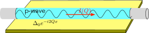
Our analysis overcomes this limitation. Indeed we investigate the effects of the superconducting phase modulation on a -wave one dimensional superconductor connected to reservoirs, as sketched in Fig.1. The system is modelled by a Kitaev chain, characterized by a hopping strength , a chemical potential , and a magnitude of the superconducting order parameter. By analyzing arbitrary parameter values, we show that, while in the regime the system remains always gapped and the role of is to merely modify the values of separating the trivial from the topological phase, a richer scenario emerges for the physically relevant range . In particular, for the phase modulation can lead the system to become a gapless -wave superconductor. By computing the current in the Kitaev model as a function of the superconducting phase modulation , we show also that, because of the -wave nature of the superconducting order parameter, the critical value determining the onset of the gapless phase is independent of the chemical potential and only depends on the superconducting order parameter. In our analysis, we determine an upper bound on current that can be driven through the system before the topological Majorana modes disappear.
The article is structured as follows. In Sec.II we describe the model and its symmetries, whereas in Sec.III we derive the general expression of the current carrying state and determine in which range of parameter values it is a conventional gapped -wave superconductor or a gapless -wave superconductor. Then, in Sec.IV we introduce the interpretation of as a synthetic dimension and we show how the current carrying state of a 1D -wave superconductor can be mapped onto the ground state of a 2D Weyl semimetal. Finally, in Sec.V we derive the current as a function of the phase modulation and of the model parameters, while in Sec.VI we summarize our results, and discuss possible implementations and future perspectives.
II Model and symmetries
Model. We consider a one-dimensional -wave superconductor modelled as an infinitely long Kitaev chain, whose Hamiltonian reads
| (1) | ||||
Here corresponds to the annihilation (creation) operator, is the chemical potential, and and are the magnitudes of the hopping amplitude and of the superconducting order parameter, respectively. The wavevector (in units of the inverse lattice spacing) characterizing the spatial modulation of the order parameter, describes a net momentum of the Cooper pair and accounts for the presence of a current flowing through the system.
Since the phenomenon we aim to describe is a bulk effect, we can safely adopt the thermodynamic limit. We assume that the number of lattice sites is large, , and adopt periodic boundary conditions (PBCs) for the system. Thus, the superconducting spatial modulation in Eq.(1), which is quantized as because of the PBCs, can effectively be treated as a continuum variable. By introducing Fourier mode operators and the Nambu spinors , one can rewrite the Hamiltonian (1) as
| (2) |
where
| (3) |
is the Bogolubov de Gennes (BdG) Hamiltonian matrix, is the identity matrix, are the Pauli matrices, and
| (4) | ||||
| (5) |
with
| (6) | ||||
| (7) |
Symmetries. By construction of the BdG formalism, the Hamiltonian (3) fulfills the particle-hole constraint
| (8) |
The application of the time-reversal transformation (anti-unitary) and the spatial inversion transformation (unitary) on the Hamiltonian Eq.(2), leads to the following relations for the BdG Hamiltonian (3)
| (9) | |||
| (10) |
showing that the presence of the spatial modulation breaks both such symmetries.
III Gapped and gapless -wave superconducting phases
The normal modes of the quadratic Hamiltonian (2), and therefore its ground state and excitations, are determined by diagonalizing the related BdG Hamiltonian (3). In order to describe the effects of the spatial modulation wavevector on the superconducting state, two remarks are in order.
First, we note that enters the BdG Hamiltonian (3) in a twofold manner. On the one hand, appears in the third component of the -vector in Eq.(5). Such a term represents a modification
| (11) |
of the bare dispersion relation of the tight-binding model [first line of Eq.(1)], which results in the reduction of the hopping parameter encoded in Eq.(6). On the other hand, introduces in the Hamiltonian (3) the additional term (4), which can be written as the difference
| (12) |
between the bare energies of two electrons in the Cooper pair frame . Such a term is odd in and causes the breaking of time-reversal and spatial inversion symmetries of the model [see Eqs.(9) and (10)].
The second remark is that, since in Eq.(3) the first term containing is proportional to the identity , the set of eigenstates of Eq.(3) is determined by the second term only. However, because the term affects the spectrum, it also determines, for each , which single-particle eigenstate is energetically more favorable and must be occupied. As a consequence, the actual many-particle state is modified by , and so are its topological properties.
To describe in details how this occurs, it is worth recalling briefly the procedure determining the the normal modes of the Hamiltonian (2). By means of the Bogolubov-Valatin unitary transformation
| (13) |
where
| (14) | ||||
| (15) |
the BdG Hamiltonian (3) can be brought to its diagonal form . The upper band and the lower band of the Kitaev model with superconducting modulation are given by
| (16) |
where . The above Eq.(8) implies that, for each -value, the two energy bands (16) are mutually related through the relation
| (17) |
whereas Eq.(9) or Eq.(10) imply that
| (18) |
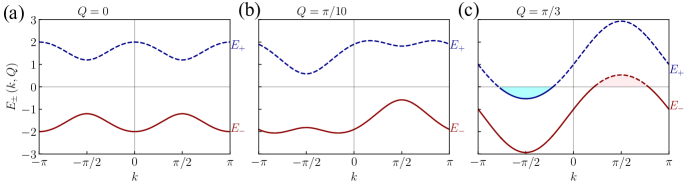
showing that the presence of makes the two bands no longer symmetric for . In Fig.2, the two bands are shown as a function of , at fixed and values, for three different values of . Panel (a) describes the customary Kitaev model: The two bands are symmetric in , the upper (lower) band is positive (negative) , and a finite direct gap exists between the two bands. As one can see from panel (b) and (c), a finite breaks the inversion symmetry [see Eq.(10)] and, when sufficiently large, it can also lead the upper band to acquire negative values, or equivalently, the lower band to become positive for the opposite values . When this occurs, the gap closes indirectly.
While the physical consequences of this behavior will be discussed in the next subsection, here we note that the Hamiltonian (2) is straightforwardly brought into its normal modes as
| (19) |
where we have exploited Eq.(17) and we have introduced Bogolubov quasi-particles , which fulfill and and are explicitly written as
| (20) | ||||
As is well known, in view of the redundancy of the Nambu spinor degrees of freedom, only one band is physically meaningful. This is why is expressed in Eq.(19) in terms of only. However, since in the following we shall have to deal both with states at and , it will be useful to use the lower band as a notation for , in view of Eq.(17).
III.1 The supercurrent carrying state
Equation (19) expresses the Hamiltonian as a collection, labelled by , of single fermionic states with energy that can be either occupied or empty. For a given value of the wavevector modulation, can in general take both positive and negative values as a function of [see Fig.2(c)]. Thus, one can partition the BZ in two regions, labelled and and defined as
| (21) |
From Eq.(19) we deduce that, if , it is energetically more convenient to leave the -th state of the upper band empty, so that the ground state fulfills . In contrast, if , the lowest energy state is realized by occupying the upper band, so that the ground state fulfills . The ground state is therefore characterized by the following conditions
| (22) |
and its energy is given by
| (23) |
as follows from Eq.(19). The conditions (22) straightforwardly imply that
| (24) |
where is a normalization constant and is a reference state to be determined. Equation (24) is the general expression of ground state of the Kitaev model in the presence of superconducting modulation. Depending on the -dependence of the spectrum, one can identify two different parameter regimes.
Gapped superconductor regime. The first regime is characterized by a finite energy gap separation between the two bands. This occurs when or, equivalently, when . In this case the sector in Eq.(21) is trivially empty, and the sector coincides with the entire BZ. The ground state (24) can then be written as , the reference state can easily be shown to coincide with the electron vacuum, , so that acquires the customary expression
| (25) |
consisting of Cooper pairs in the bulk only. It can be shown (see App.A) that this regime exists for the following three parameter ranges
| (26) |
The case discussed in [59, 58] is a subcase of the second parameter range.
Gapless superconductor regime. This regime occurs when (or equivalently ) for some values of , i.e. when the sector in Eq.(21) is not empty. Recalling the expression (16), the condition for such gapless superconducting regime to occur are determined by imposing that the condition is fulfilled for some ’s. Some lengthy but straightforward algebra [see Appendix A] leads to conclude that such a situation occurs if and only if the following parameter conditions are fulfilled
| (27) |
Because now the sector is not empty, the operators appearing in the general Eq.(24) yield some different features with respect to the conventional gapped superconductor, as can be suitably recognized by re-expressing Eq.(24) in terms of fermionic operators . To this purpose, we introduce one further partitioning of the sector defined in Eq.(21), where the two subsectors and are identified by inspecting the sign of or, equivalently the sign of , in view of Eq.(17). Explicitly, one can partition the BZ as , where
| (28) |
Note that is just another notation for . In this case, one can show [see Appendix B] that and that can be rewritten in terms of the operators as
| (29) |
As compared to the gapped superconductor (25), the gapless superconducting state (29) contains not only Cooper pairs ( sector), but also a pocket of unpaired electrons ( sector), and a pocket of unpaired holes ( sector). An illustrative example is shown in Fig.2(c), where the unpaired electron and hole pockets are highlighted in cyan and pink colors, respectively. In this regime the superconducting order parameter is no longer interpreted as the gap. Yet, the energy (23) of the state (29) is still lower than the state of a fully normal state (). Interestingly, the structure of Eq.(29) is similar to the one found for neutral superfluids with orbital angular momentum[60, 61]. Here, however, the -wave nature of the order parameter implies significantly different features, as will be explained in Sec.IV.
As a consequence of its mixed structure, exhibits normal and anomalous correlations depending on the -sectors. Explicitly, one can show [see Appendix B] that the normal correlation read
| (30) |
| (31) |
while the anomalous correlators are
| (32) |
The elementary excitations above the ground state are given in Appendix C.
Before concluding this section, a remark is in order. In partitioning the BZ, we have not mentioned the case . This corresponds to a degeneracy in the spectrum of the Hamiltonian (19). Thus, although one ground state can still be written in the forms (25) or (29), it is degenerate with a state where an additional single fermion is present. In a closed system, these two ground states have different fermion parity[62]. However, if the system is contacted to reservoirs inducing a current flow, as is the case of interest here, fermion leakage makes both states equally probable. Thus, such a single fermion state merely represents here a zero-measure support set in the BZ.
IV Effective 2D fermion model and Lifshitz transition
We now want to discuss how the the presence of the superconducting phase modulation affects the topological aspects of the Kitaev model.
When the system is in the gapped regime, although changes quantitatively the spectrum with respect to the case [compare e.g. Figs.2(a) and (b)], it does not alter the occupancy of bands because . The ground state consists of a completely empty upper band or, equivalently, of a completely filled lower band . Then, one can characterize through the topological index associated to the lower band. Notice that this case, described in Ref.[59], follows exactly the same lines as the customary case, and the role of is to merely renormalize the hopping amplitude appearing in Eq.(6).
The situation is different in the gapless regime, where , for some ’s. For such -states the presence of the -term in Eq.(16) alters the occupancy. In the ground state not all the lower band states are occupied, and the approach adopted to topologically classify gapped phases cannot be straightforwardly applied to gapless phases.
However, the presence of the superconducting order parameter modulation offers the opportunity to adopt a different perspective. The idea is that can be regarded as the wavevector an extra synthetic dimension, in addition to . In this way a 1D superconductor with superconducting phase modulation can be associated to a 2D fermionic model. The Lifshitz transitions[44] occurring in the topology of the Fermi surface of the half-filled 2D model enable one to characterize the ground state phases of the 1D superconductor. In particular, we shall show that the -wave superconductor is associated to a 2D WSM, which can be in type-I or type-II regime.
IV.1 Effective 2D fermion model
We start by observing that, although the envisaged system is one-dimensional, the Hamiltonian (1) is -periodic in the superconducting order parameter modulation . As a consequence, the Bogolubov de Gennes Hamiltonian Eq.(3) of the Kitaev chain with the superconducting phase modulation can also be interpreted as the first-quantized Hamiltonian of a two-dimensional system with a sublattice or orbital degree of freedom
| (33) |
where is the wavevector lying on a torus. In Appendix D, we provide the explicit expression of in real space. The spectrum of this fictitious 2D model is determined by and is therefore the same as the one of the Kitaev model with a superconducting phase modulation. Two remarks are in order.
First, the 2D model contains twice the degrees of freedom of the Kitaev model. Indeed, while in Eq.(33) the spinors corresponds to two actual independent sublattice degrees of freedom and both bands and are physical, in the Kitaev model such two spectral bands are not independent in view of the redundancy intrinsic in the Nambu spinors, so that only one is actually physical.
The second remark is related to symmetries. In such a dimensional promotion, the role of symmetries is interchanged. In particular, while for the Kitaev chain the relations (9) and (10) encode broken time-reversal and inversion symmetries, for the associated 2D model Eq.(33) they represent fulfilled symmetries. Recalling that , these symmetries imply
| (34) |
and
| (35) |
respectively, and yield the relation (18). In contrast, while for the 1D Kitaev chain Eq.(8) is a built-in particle-hole symmetry stemming from the BdG formalism, it represents an anisotropy constraint for the 2D model, which implies
| (36) |
and is responsible for the mutual relation (17) between the two bands.
IV.2 Lifshitz transition
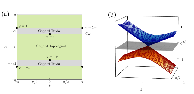
The Fermi surface is defined in the 2D BZ as the set of such that the eigenvalues fulfill or . In particular, we shall inspect the possibility that the Fermi surface contains nodes, where the two bands and touch, i.e. . In view of Eq.(16), this equivalently corresponds to the set of four equations () for two unknown coordinates of . From symmetry arguments based on Eqs.(34), (35) and the constraint (36), one can deduce whether and how such nodes occur. Indeed, the fact that both and symmetries hold implies , which eliminates one equation. Then, from Eq.(36) and either (34) or (35) we see that must be odd in the component, and even in -component of . This is the case for the Kitaev model, because of the -wave symmetry of the superconducting order parameter (7). This means that the nodes can only occur at or , and that they exist as long as [see Eq.(5)] can vanish, which is the case only if . Then, the nodes are Weyl nodes that are locally protected by and symmetries. Their location
| (37) |
where
| (38) |
depends on the chemical potential and not on the value of . The WSM nature (Type-I vs Type-II) is determined by the behavior of the term. In the vicinity of the Weyl node (with ), the Hamiltonian in Eq.(3) is well approximated by a low energy Hamiltonian
| (39) |
where and correspond to the deviations in momentum from , and
| (40) |
Each Weyl node carries a vortex, as can be seen from by computing the lower band Berry phase over a contour enclosing the Weyl node in the momentum space
| (41) |
where is the Berry potential and is a diagonal matrix with components given by (40), near the Weyl node .
Going back to the full BdG Hamiltonian (3) and taking into account the explicit expressions (4) and (5), we deduce that for the Kitaev model three scenarios can emerge in the Fermi surface of the associated 2D model, depending on the Kitaev model parameter ranges:
1) Type-I WSM phase. In the parameter range
| (42) |
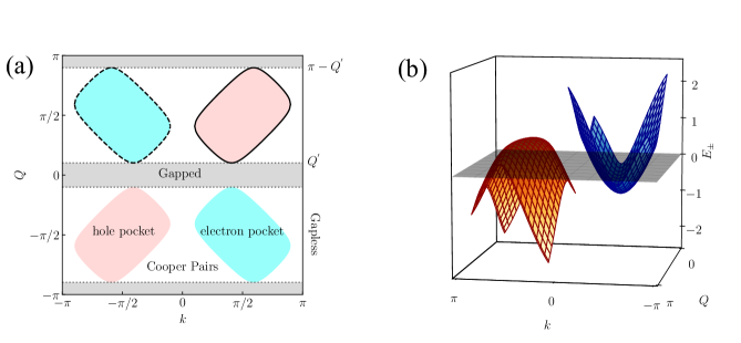
the Fermi surface consists of four isolated Weyl nodes , where the two bands and touch, while and otherwise (. In this regime the -term in the Hamiltonian modifies the spectrum but not the occupancy of the bands, and the model (33) corresponds to a two-dimensional Type-I WSM with a Fermi level at . The Weyl nodes, shown as black bullets in Fig.3(a) and the type-I band dispersion relation is shown in Fig.3(b).
We shall now argue that this Fermi surface of the 2D model enables us to recover the topological classification of the Kitaev model and to determine the region of parameters where Majorana fermions occur, in the presence of the superconducting phase modulation. Indeed in this regime the lower band of the Hamiltonian is completely filled, while the upper band is completely empty. Thus, for each cut of the band structure at a fixed away from the Weyl nodes (), one obtains a gapped one-dimensional insulator, which can be classified in the topological class D[63], since it only exhibits the particle-hole symmetry (8). The related topological invariant is the Zak-Berry phase of the lower band,
| (43) |
which is quantized in integer multiples of due to the particle-hole symmetry or, equivalently, through[64]
| (44) | |||||
Trivial phases () correspond to the condition , whereas topological phases () correspond to and, for the case , are depicted as grey and green regions in Fig.3, respectively. Thus, in the regime (42) the range of -values where Majorana exist is controlled by the chemical potential , and is independent of the value of . The condition (42) includes the case studied in Ref.[59]. In the case , Eq.(42) reduces to
| (45) |
which, for the physically realistic regime , represents a very narrow range of chemical potential value for this regime to exist.
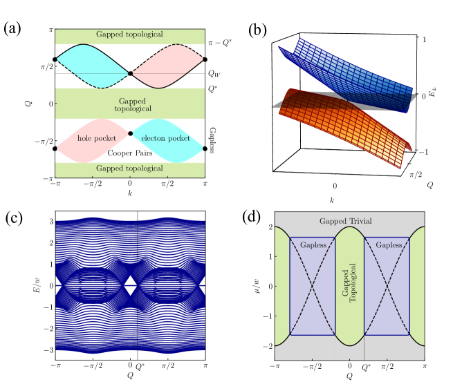
2) Type-II WSM phase. Let us now focus on the regime
| (46) |
which is physically most realistic, as the superconducting order parameter is typically much smaller than the bandwidth parameter . The scenario of the Fermi surface
is depicted in Fig.4(a). The Weyl nodes are still located in the positions given by Eqs.(37). However, they are now Type-II nodes, as shown in Fig.4(b), since the Fermi surface of the 2D model exhibits pockets of unpaired electrons and holes, which correspond to the regions where the magnitude of the -term overcomes the -term. Note that electron and hole pockets are mutually mirrors of each other for , as a straightforward consequence of the relation (17) originating from the particle-hole constraint Eq.(8) of the BdG formalism.
The three panels of Fig.2 represent three cuts of band in the 2D BZ shown in Fig.4(a), at different values of , where one can see the Lifshitz transition from the gapped phase in panels (a)-(b) (empty Fermi surface) to the gapless phase in panel (c) (appearance of electron and hole pockets), where the ground state of the Kitaev model is given by Eq.(29).
The fermion and hole pockets, identified by and , respectively, cross of the Weyl nodes. As one can see from Fig.4(b), in the range , where
| (47) |
the ground state is gapless, and it exhibits Cooper pairs, unpaired fermions and holes. In contrast, in the range and , it is gapped and topological. Indeed the spectrum plotted in Fig.4(c) for a finite-size Kitaev chain of sites, shows the existence of zero-energy Majorana bound states in such range of values.
A striking difference emerges with respect to the regime 1) described above. In that case the range of -values, where the gapped topological phase exists is purely determined by the chemical potential and is independent of the superconducting order parameter , provided the latter is large enough to fulfill the energy range (42). This holds, in particular, for any . Indeed the topological phase –green region in Figs.3(a)– is determined by the -dependent location of the Weyl nodes only. In contrast, for , and in particular in the regime 2) specified by Eq.(46), the -boundaries for the topological phases are determined by through the critical value (47), and are independent of the chemical potential. As shown in Fig.4(a), the topological phase (green region) is no longer determined by the location of the Weyl nodes, but by the boundaries of the electron and hole pockets. The comparison between the two regimes is clearly illustrated in Fig.4(d), where the phase diagram of the Kitaev model in the regime 2) is shown as a function of and , while the dashed lines represent the phase diagram for the regime 1). At each fixed value of , the topological region (green area) is smaller than in regime 1) because the system enters the gapless phase (violet color).
3) no Fermi surface. When , the two Weyl nodes of each -th pair merge. Then, in the regime
| (48) |
the Weyl node equation cannot be fulfilled [see Eqs.(5) and (6)], the Weyl nodes disappear and the Fermi surface is an empty set. This corresponds to the situation where and, in terms of a -cut, this describes a topologically trivial phase.
IV.3 Zero energy modes
In open boundary conditions for the 2D model, both regimes 1) and 2) exhibit localized Fermi “arc” states, which form effectively one-dimensional zero-energy bands, parametrized by the crystal momentum along the infinite direction. We will consider for clarity a single boundary at .
Let us start from the Type-I Weyl phase, in the parameter regime (42). For , we find an arc connecting the projections of the nodes and containing the point and an arc connecting the projections of the nodes containing , see Fig.3. Conversely, for , the projection of the nodes is closer to the point than the projection of the nodes : in this situation, there is an arc connecting across the BZ and an arc connecting including the origin. In terms of the 1D model, the endpoints signal the transition between the topological and the trivial phase 111Note that in the Weyl-I regime (42), if the denominator of is positive (topological phase), the argument of the square root in the numerator is also positive.. In Appendix E, we follow an established route for constructing Fermi arcs in Weyl Hamiltonian [66, 67, 68, 69]. Linearizing the Hamiltonian (33) in , one finds localized eigenstates in the form
| (49) |
where
| (50) |
Here, , while
| (51) |
represents the penetration depth. It is readily observed that this quantity diverges at the arc ends.
In the Type-II Weyl phase (46), we see from Fig.4 the emergence of electron/hole pockets in the bulk. We find that the Fermi arcs are still described by (49), but now connect the projections of the bulk electron and hole pockets onto the surface BZ. In particular, the edge states have support between the values given in (47), including the origin , and outside the points [see Appendix E]. In terms of the 1D model, these points signal the transition between the topological gapped phase and the gapless superconductor phase, see Fig.4. In contrast to the previous regime, the penetration length (51) vanishes at the arc ends. A derivation and a plot of (51) in the two regimes can be found in Appendix E.
The two components of the wavefunction (50) represent in the 2D model the weights on the and sublattices or orbital degrees of freedom. However, they are directly interpreted as the electron (top) and hole (bottom) components in the 1D superconductor model. Therefore, the wavefunction (50) describes the Majorana edge mode of the 1D TS associated to the Fermi arc (49) for the Kitaev chain with a -modulation of its superconducting order parameter. We recall that the 2D fermionic system (33) exhibits twice the number of degrees of freedom as the original Kitaev model, for which only a half of the spectrum (say, the upper band) can be retained. This is particularly evident in a slab geometry with a finite size along the -direction. In the 2D fermionic model, two fermionic states appear around , and can be seen as symmetric and antisymmetric combinations of the Fermi “arcs” localized at the two edges. However, in the 1D Kitaev model only one fermionic state is physical and it consists of two Majorana quasi-particles localized at the system edges.
IV.4 Comparison with the case of a -wave superconductor
Also a conventional -wave superconductor carrying a current exhibits a modulation of the superconducting order parameter, and can enter a gapless phase. Here we want to highlight the difference from the -wave superconductor from the point of view of the mapping to a 2D model.
In a -wave superconductor the order parameter term in the presence of a spatial modulation is . By introducing a Nambu spinor , the BCS Hamiltonian appears to be the sum of two decoupled sectors sharing the same BdG Hamiltonian , where is again given by Eq.(4), while
| (52) |
with still given by Eq.(6). Similarly to what described in Sec.IV.1 for the Kitaev model, one can apply a mapping to a 2D (spinful) fermionic model, where spin is a degeneracy degree of freedom for the two bands. The resulting Fermi surface, shown in Fig.5(a), exhibits two crucial differences with respect to the Kitaev case [see Fig.4(a)]. First, the BCS model does not exhibit any node, since the vector in Eq.(52) can never vanish, as is clear from Eq.(52). As a related consequence, gapped phases are always topologically trivial, since the Bloch vector spans a trivial line in the - plane, as expected for the BCS model.
Similarly to the Kitaev case, the presence of the term stemming from the superconducting modulation leads to the emergence of gapless superconducting phases, which in this case exist when both the conditions and are fulfilled, where . Note that these boundaries are dependent on both and , while in the Kitaev case they are -independent. Importantly, the boundaries of the electron and hole pockets in the BCS case are topologically different from the ones of Fig.4(a). Indeed, while in the Kitaev model the solid and dashed boundaries run over the entire -circle of the BZ, in the BCS model they remain localized to the finite portion specified above.
Such a topological difference in the Fermi surfaces of -wave and -wave gapless superconductors can be characterized in terms of the homology group of 1-cycles[70], i.e. closed circuits on the 2D BZ torus . A closed Fermi surface circuit is identified by a mapping and can be classified according to two topological indices , defined as the winding numbers related to the two orthogonal circuit direction along the torus
| (53) | |||||
| (54) |
Let us now compare the Fermi surface closed circuits of the -wave superconductor and -wave superconductor. In the former case, consists of the four curves that in Figs.4(a) delimit the electron and hole pockets. In particular, the ones highlighted as solid or dashed are given by
| (55) |
respectively. Note that, at the crossing at the Weyl nodes, the solid and the dashed line are uniquely identified through the continuity of the eigenvectors related to the vanishing eigenvalues . As a consequence, the Kitaev Fermi surface winds around the -direction and therefore belongs to the topological class. In contrast, for the -wave superconductor described, the BCS Fermi surface illustrated in Fig.5(a) is always localized and belongs to the class, which is homotopically equivalent to a point.
Importantly, these different topological classes are closely related to the presence or absence of nodes in the 2D Fermi surface. Indeed in the Kitaev case the electron and hole pocket must necessarily go through the Weyl nodes, located at and , because the -wave superconducting order parameter is odd in . In a -wave superconductor, instead, the absence of nodes makes the Fermi surface consist of localized curves.
Thus, in terms of the associated the 2D model, a 1D -wave superconductor corresponds to either a 2D insulator or a 2D conventional semimetal, depending on the parameter range [see Fig.5(b)]. In contrast, a 1D -wave superconductor corresponds to a trivial 2D insulator or a 2D Type-I/Type-II WSM [see Fig.3(a) and Fig.4(a)].
V -dependence of the current
We now want to analyze the behavior of the current carried by the ground state . As is well known, the operator describing the current flowing through the site is given by , where is the electron charge. The spatial conservation of the expectation values follows from charge conservation, and one can show 222By exploiting the current conservation at stationarity, one can write that . Then, by applying the gauge transformation , one can shift the phase modulation in the superconducting term and set it into the hopping term , whence one has , and therefore Eq.(56). that
| (56) |
Furthermore, exploiting the expression (23) and taking the thermodynamic limit , one obtains the current as a function of the superconducting modulation
where
| (58) |
is odd function of , called spectral asymmetry[60], which identifies the three sectors (28) as well as the relative magnitudes of and in Eqs.(4)-(5), namely
| (59) |
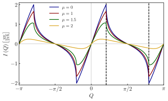
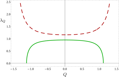
Figure 6 shows the current in units of as a function of , for different values of the chemical potential . The golden curve illustrates the case, where the model parameters fulfill the condition (45), corresponding to the Type-I phase for the WSM. The current is a smooth function of . In contrast, the blue and red curves in Fig.6 refer to cases where the condition (46) is fulfilled, corresponding to the Type-II phase for the associated WSM. As one can see, the current exhibits sharp cusps at and [see Eq.(47)], which are the hallmark of the transition from the topological gapped to the gapless superconducting phase, where unpaired fermions and holes appear in the ground state [see Fig.4]. The location of the cusp is independent of the value of the chemical potential. Note also that the cusps correspond to the maximal current values, whereas the current always vanishes at , for any value of and . From a mathematical viewpoint, this stems from the fact that the the current (V) is an odd function of the deviation . From a physical viewpoint, for the renormalized hopping term vanishes, the bare band becomes flat, and unpaired fermions cannot carry any current, while the crystal momentum of the Cooper pairs equals its opposite , implying also that the Cooper pair current vanishes.
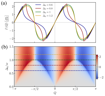
The qualitatively different behavior of in the Type-I vs Type-II parameter ranges (45) and (46) is further highlighted in Fig.7, which displays the current (56) as a function of , at , for different values of the superconducting order parameter . As one can see from panel , for the 1D Kitaev model is in the WSM Type-I parameter range and the current exhibits a smooth behavior as a function of , whereas for the Kitaev chain enters the WSM Type-II phase and the cusps clearly appear in the current. Panel (b) shows a density plot of the current as a function of , where the horizontal dashed lines represents the four cuts shown in panel (a).
For the special case , it is also possible to determine an analytical expression for the current [see Appendix F for details], whence one can show that for the current exhibit a linear behavior as a function of
| (60) |
which represents the current carrier by Cooper pairs with momentum and charge . Similarly, for , the maximal current reached at the cusp is
| (61) |
For one obtains a maximal current lower than the one at , as can be seen from Fig.6. Thus, Eq.(61) represents the maximal current that the TS, characterized by a given , can sustain in the topological phase, i.e. right at the transition to the gapless phase.
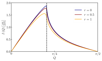
Effects of disorder.
We have also analyzed the effects of disorder on the behavior of the current. Specifically, we have considered a disordered on-site potential, which we have accounted for by replacing the constant chemical potential in the Hamiltonian (1) with , where is the disorder strength parameter and is a uniformly distributed random number. Figure 8 shows the -dependence of the current for , , for three values of disorder strength, (clean case), (moderate disorder) and (strong disorder). Each curve corresponds to an average over a large number of disorder realizations. As far as the disorder remains moderate, the cusp behavior of the current at (vertical dashed line) remains robust, and the only effect of disorder is to reduce a bit the magnitude of the current. Only for strong disorder the curve smoothens and the cusp disappears.
VI Discussion and Conclusions
In this paper we have investigated the effects of the spatial modulation emerging in the superconducting order parameter when a topological -wave superconductor carries a current flow. By modelling the system with a Kitaev chain, we have analyzed the properties of the current carrying state for arbitrary values of the model parameters, including the physically realistic regime .
We have demonstrated that, by treating the -modulation as the wavevector related of an extra synthetic dimension, it is possible to establish a mapping between the stationary nonequilibrium state of the 1D superconductor and the ground state of a 2D WSM. The Lifshitz transitions emerging in the Fermi surface of the 2D model as a function of the model parameters identify different phases of the topological superconductor travelled by a current. Exploiting such a mapping, we have also constructed the expression (49) of the Fermi “arc” in the 2D WSM and the Majorana quasi-particle (50) in the corresponding current-biased 1D TS.
In particular, in the regime identified by Eq.(42), the 2D WSM is in its Type-I phase with four Weyl nodes, whose location depends only on the chemical potential through the value of [see Eq.(38)], and determines the separation between gapped topological and trivial phases of the Kitaev chain. The Fermi “arcs” (49) correspond to the Majorana quasi-particles (50) emerging in the topological phase (see Fig.4), and their penetration length (51) diverges at and . Note that, for realistic values , the regime Eq.(45) of Type-I WSM reduces to a small chemical potential range. In contrast, when the model parameters fulfill the broader range Eq.(46), the 2D system is a Type-II WSM. In this case electron and hole pockets correspond to the gapless superconductor phases of the Kitaev chain, where Cooper pairs coexist with unpaired electrons and holes (see Fig.5). In this case, the -range where the gapped topological phase exists is no longer determined by the location of the Weyl nodes. Instead, it depends on only, through the value of given by Eq.(47). Notably, the penetration length of the Majorana edge mode vanishes at such transition value between the topological gapped and the gapless phase of the Kitaev model.
Furthermore, we have highlighted the difference with respect to the -wave superconductor, where the associated 2D fermionic model can be either a trivial insulator or a conventional semimetal (see Fig.6). The difference between the 2D Fermi surfaces corresponding to the -wave and -wave superconductors are shown to correspond to two different classes of the homology group of closed circuits along the 2D BZ.
Finally, by computing the current flowing through a the Kitaev chain, we have shown in Figs.6 and 7 that it exhibits a sharp cusp at the critical value , corresponding to the transition between the gapped and the gapless phase illustrated in Fig.5(a) and (d). Importantly, the value of given in Eq.(47) is independent of the chemical potential variations and is robust to disorder (see Fig.8). Moreover, it determines the maximal current [see Eq.(61)] that the -wave topological superconductor can sustain in its topological phase where Majorana quasi-particles exist. Before concluding, we also would like to discuss some possible implementations of the model investigated here, and to outline some future perspectives of our results.
Implementations. One of the most explored implementations of 1D topological superconductors are nanowires with strong spin-orbit coupling, such as InSb and InAs, proximized by a thin conventional superconducting layer (e.g. Al or Nb) and exposed to a longitudinal magnetic field. One of the signatures that seems to be compatible with the existence of MQPs is a pronounced zero-bias peak observed in the conductance in electron tunneling experiments. However, the question whether such a peak is actually due to MQPs or to other nontopological effects is still under debate. Here, from our result Eq.(61), we can estimate the maximal current that the 1D -wave superconductor can sustain before entering the gapless phase, where Majorana quasi-particles are absent. Using the estimated values for the induced gap in InSb nanowires[35, 36, 38] and for InAs nanowires[37], one finds . This range of values is of the same order of magnitude as the typical current in nanowire experiments.[72, 73, 25]
Future perspectives. Our analysis has focussed on the the mapping between a 1D TS and a 2D WSM. However, the idea of harnessing the phase modulation as a synthetic dimension is actually quite general and can apply to higher dimensional cases. We thus can expect that a 2D TS where a current flowing in a specific direction can be mapped to 3D WSM. Our results thus pave the way to interpret the properties of WSMs as an observation of lower dimensional TSs with a current flow.
Acknowledgements.
F.D. acknowledges financial support from the NEThEQS PRIN 2022 Project (code 2022B9P8LN) and fruitful discussions with Mario Trigiante. F.G.M.C. acknowledges financial support from ICSC—Centro Nazionale di Ricerca in High-Performance Computing, Big Data, and Quantum Computing (Spoke 7), funded by European Union—Next Generation EU.Appendix A Parameter ranges of gapless and gapped phases of the Kitaev model
Here we provide details to determine the range of parameters , and characterizing the gapped and gapless phases of the Kitaev model. Recalling that the spectrum Eq.(16) is determined by the functions and [see Eqs.(4) and (5) in the Main Text], we shall identify here the gapless and gapped phases.
Gapless phase. The gapless phase of the Kitaev model is determined by the condition
| (62) |
Introducing the quantity
where , and recalling the expressions (4) and (5), the inequality (62) amounts to requiring
| (64) |
At any given the inequality Eq.(64) is fulfilled only in the range
| (65) |
provided that the two roots
| (66) |
of the equality are real. Thus, the requirement implies
| (67) |
which is the first Eq.(27) given in the Main Text. Then, we observe that, by introducing the following angle
| (68) |
and by denoting , the roots (66) can be rewritten as
| (69) |
This implies that , i.e. that the solutions (65) always belong to the physically acceptable range for the variable . Thus, at any given , the range of values for which unpaired electrons and holes exist is given by
| (70) |
Because in Eq.(70) the extremal values are always reached by for some value of , the actual range of for which unpaired electrons and holes are present is precisely
| (71) |
i.e. . This is the second Eq.(27) given in the Main Text. In turn, it also determines the onset value (47) for the appearance of the electron and hole pockets.
Gapped phase. The Kitaev model is gapped if
| (72) |
i.e. if
| (73) |
where is given in Eq.(LABEL:Phi-def). One can now distinguish two ranges of chemical potential. For , it is straightforward to realize from Eq.(LABEL:Phi-def) that the gapped phase condition Eq.(73) is fulfilled . This is the case i) in Eq.(26). When , Eq.(73) is fulfilled in two subcases. The first one is when has no real roots for any , which occurs for the parameter range ii) given in Eq.(26). The second one occurs when has two real roots, i.e. for . In that case, for a given , the inequality is fulfilled for and , where the roots are given by Eq.(69). However, Eq.(73) requires that this holds for any , this implies that , i.e. , whence one obtains the case iii) given in Eq.(26).
Appendix B Ground State
Here we show that the general expression (24) of the current carrying ground state implies the equivalent expression (29). Indeed, by rewriting Eq.(24) using the partitioning (28) one can write the ground state as
| (74) |
By changing the in the ’s of the sector one can equivalently write
| (75) | |||||
where we have used the relation following from Eqs.(20). From Eq.(75) we deduce that the reference state is . Finally, by noticing that , one obtains the normalized state Eq.(29).
Appendix C Elementary Excitations
From Eq.(19) and from the properties (21) characterizing the ground state, it is straightforward to realize that the elementary excitations of the system are characterized by an energy with respect to the ground state energy (23), and are given by for , and for . Moreover, as we have seen above, the BZ can be partitioned in three sectors , and one can identify three types of elementary excitations
| (80) | |||||
| (81) | |||||
| (82) |
Using Eq.(20) we can see that the first type of excitation () takes the form
| (88) | |||||
where, as compared to the ground state (29), an empty fermionic state at and a filled fermionic state at are replaced by a cooper pair . Notably, such type of Cooper pair is orthogonal to the Cooper pair characterizing the ground state, i.e.
| (89) |
For the sector the excited state reads
| (95) | |||||||
where, as compared to the ground state (29), a single fermionic state at and an empty fermionic state at are replaced by a cooper pair of the same type as the ones characterizing the ground state in the sector. Finally for the sector
| (100) | |||||
where, as compared to the ground state (29), a Cooper pair in the sector has been replaced by one single fermion.
Appendix D Lattice model
In this Appendix, we provide additional details about the 2D lattice model described by the Hamiltonian (33). The Hamiltonian contained therein can be written in the form
| (101) |
After Fourier transforming to real space, one obtains
| (102) | |||||
and the various terms are sketched in Fig.9. The and spots represent two different orbitals in the same site or two different sites in the same unit cell.
Although we are presently unaware of a material described by the above Hamiltonian, the recent proposals of realizations of 2D WSMs with ultracold atoms[18], suggest that its realization in the near future with synthetic materials, e.g., cold-atomic or photonic lattices could be possible.
Appendix E Fermi arcs
In this Appendix, we consider the 2D Weyl Hamiltonian in Sec. IV with a boundary in the direction , say, at , while remaining infinite in the direction . We look for the surface states, and aim in particular at determining their support in the surface Brillouin zone. To this end, we will focus on the low energy Hamiltonian expanding around the Weyl nodes. In the Type-I phase, in order to describe the “arc” joining the projection of the Weyl nodes , one obtains
| (103) |
which contains the first term in the momentum expansion of (33) around . The same expansion is used in the Type-II phase, but the arc joins now the electron/hole pockets enclosing the nodes. The most general boundary condition ensuring the self-adjointness of (103) can be derived by taking two arbitrary spinors and and imposing that in the chosen geometry [66]. In the absence of the phase modulation , this would imply the condition normally derived for Type-I Weyl semimetals [67]. Here instead, we obtain the constraint
| (104) |
provided and are well-behaved for . We note that, taking , the above equation implies that the density current across the boundary vanishes. It also implies that the state on the surface must take the form
| (105) |
where the phase must be a function of and satisfy
| (106) |
The latter equation directly implies the expression of given in Sec. IV.2 and, for , reduces to the eigenstate of with positive eigenvalue. This is the familiar form describing a straight “arc” in Type-I Weyl semimetals or the Majorana end mode in the Kitaev model. Taking an Ansatz wavefunction in the form (50) with an unspecified in the exponent, it can be directly verified applying the Hamiltonian (103) that this represents a zero-energy eigenstate only if the penetration length is a function of the momentum and the condition
| (107) |
is satisfied. Finally one solves for the penetration length and the relation selects the branch of the solution for from the condition that along the arc. To this end, we recall that, in the Weyl-I phase, the arc connects the projection of the nodes through the origin for , i.e., , while for the arc winds instead across the BZ and . The same procedure can be readily applied to the Type-II Weyl phase, with the important difference that there appear bulk states around the Weyl nodes. Therefore, the arc support is shorter and spans the interval for , while it joins and including the point for .
Similarly, one can describe the “arc” connecting the projection of the Weyl nodes by considering the expansion of (33) around . It is readily verified that this Hamiltonian can be formally obtained from by exchanging and . By repeating the steps above, the surface state must once again reduce to (105) on the boundary and the form (50) describes a zero-energy state under imposing
| (108) |
Solving (107) and (108) for , the branch of the phase is again selected by the condition .
To this end, it is important to notice that the Fermi arc support includes if , while it includes the origin for .
Joining the above considerations, one finds the expression (51) in the main text, also represented in Fig. 10 for two sample values of parameters in the two Weyl phases.
Appendix F Analytical expression for the current at
Here we show that, starting from the general expression (V) for the current, for the special case we can derive an analytical expression of that holds for arbitrary values of . We first observe that, for , the function (LABEL:Phi-def) determining gapless and gapped region reduces to . Then, taking into account the sign of [see Eq.(4)], the conditions (59) enable one to determine the values of the spectral asymmetry over the Brillouin zone
| (109) |
where
| (110) |
The expression (V) of the current consists of two contributions, one proportional to , which represents the current carried by unpaired fermions and holes, and a second termn proportional to , that represents the supercurrent due to Cooper pairs. Let us start by determining the former contribution. Indentifying through Eq.(109) the -regions where , one finds
Recalling Eq.(110), one obtains
| (112) | |||||||
Let us now consider the current associated to Cooper pairs (). From the expression (LABEL:current_continuum-v0), the current associated to the Cooper pairs is
| (113) | |||||
By introducing the quantity
| (114) |
and by exploiting the fact that and are even functions of , some straightforward algebra leads one to write
| (115) | |||||||
One can now identify from Eq.(109) the regions with and write
| (116) | |||||
Let us now focus on the two integrals appearing in the first term. We notice that, by changing the integration variable in the second integral, the latter turns out to be equal to the first one. Similarly, the integral appearing in the second term can be written as twice the integral from to . This enables one to rewrite
| (117) | |||||
where , and are incomplete elliptic functions, while and . Finally, exploiting the properties of the Elliptic integrals and for , and combining together the contributions (112) and (117), one finally obtains the current at
| (118) |
where is Eq.(114), and is Eq.(110). The current near and for gives
| (119) |
and to leading order the slope depends only on the bandwidth parameter .
References
- Shekhar et al. [2015] C. Shekhar, A. K. Nayak, Y. Sun, M. Schmidt, M. Nicklas, I. Leermakers, U. Zeitler, Y. Skourski, J. Wosnitza, Z. Liu, et al., Extremely large magnetoresistance and ultrahigh mobility in the topological Weyl semimetal candidate NbP, Nature Physics 11, 645–649 (2015).
- Armitage et al. [2018] N. P. Armitage, E. J. Mele, and A. Vishwanath, Weyl and Dirac semimetals in three-dimensional solids, Rev. Mod. Phys. 90, 015001 (2018).
- Burkov and Balents [2011] A. A. Burkov and L. Balents, Weyl semimetal in a topological insulator multilayer, Phys. Rev. Lett. 107, 127205 (2011).
- Hasan et al. [2017] M. Z. Hasan, S.-Y. Xu, I. Belopolski, and S.-M. Huang, Discovery of Weyl fermion semimetals and topological Fermi arc states, Annual Review of Condensed Matter Physics 8, 289–309 (2017).
- Soluyanov et al. [2015] A. A. Soluyanov, D. Gresch, Z. Wang, Q. Wu, M. Troyer, X. Dai, and B. A. Bernevig, Type-II Weyl semimetals, Nature 527, 495–498 (2015).
- Wang et al. [2016] C. Wang, Y. Zhang, J. Huang, S. Nie, G. Liu, A. Liang, Y. Zhang, B. Shen, J. Liu, C. Hu, Y. Ding, D. Liu, Y. Hu, S. He, L. Zhao, L. Yu, J. Hu, J. Wei, Z. Mao, Y. Shi, X. Jia, F. Zhang, S. Zhang, F. Yang, Z. Wang, Q. Peng, H. Weng, X. Dai, Z. Fang, Z. Xu, C. Chen, and X. J. Zhou, Observation of Fermi arc and its connection with bulk states in the candidate type-II Weyl semimetal WTe2, Phys. Rev. B 94, 241119 (2016).
- Li et al. [2017] P. Li, Y. Wen, X. He, Q. Zhang, C. Xia, Z.-M. Yu, S. A. Yang, Z. Zhu, H. N. Alshareef, and X.-X. Zhang, Evidence for topological Type-II Weyl semimetal WTe2, Nature communications 8, 2150 (2017).
- Yao et al. [2019] M.-Y. Yao, N. Xu, Q. S. Wu, G. Autès, N. Kumar, V. N. Strocov, N. C. Plumb, M. Radovic, O. V. Yazyev, C. Felser, J. Mesot, and M. Shi, Observation of Weyl nodes in robust type-II Weyl semimetal WP2, Phys. Rev. Lett. 122, 176402 (2019).
- Bovenzi et al. [2018] N. Bovenzi, M. Breitkreiz, T. E. O’Brien, J. Tworzydło, and C. W. J. Beenakker, Twisted Fermi surface of a thin-film Weyl semimetal, New Journal of Physics 20, 023023 (2018).
- Breitkreiz and Brouwer [2019] M. Breitkreiz and P. W. Brouwer, Large contribution of Fermi arcs to the conductivity of topological metals, Phys. Rev. Lett. 123, 066804 (2019).
- Buccheri et al. [2022a] F. Buccheri, R. Egger, and A. De Martino, Transport, refraction, and interface arcs in junctions of Weyl semimetals, Phys. Rev. B 106, 045413 (2022a).
- Xu et al. [2015] S.-Y. Xu, I. Belopolski, N. Alidoust, M. Neupane, G. Bian, C. Zhang, R. Sankar, G. Chang, Z. Yuan, C.-C. Lee, et al., Discovery of a Weyl fermion semimetal and topological Fermi arcs, Science 349, 613–617 (2015).
- Wu et al. [2016] Y. Wu, D. Mou, N. H. Jo, K. Sun, L. Huang, S. L. Bud’ko, P. C. Canfield, and A. Kaminski, Observation of Fermi arcs in the type-II Weyl semimetal candidate WTe2, Physical Review B 94, 121113 (2016).
- Tamai et al. [2016] A. Tamai, Q. Wu, I. Cucchi, F. Y. Bruno, S. Riccò, T. K. Kim, M. Hoesch, C. Barreteau, E. Giannini, C. Besnard, et al., Fermi arcs and their topological character in the candidate Type-II Weyl semimetal MoTe2, Phys. Rev. X 6, 031021 (2016).
- Morali et al. [2019] N. Morali, R. Batabyal, P. K. Nag, E. Liu, Q. Xu, Y. Sun, B. Yan, C. Felser, N. Avraham, and H. Beidenkopf, Fermi-arc diversity on surface terminations of the magnetic Weyl semimetal Co3Sn2S2, Science 365, 1286–1291 (2019).
- Hao and Ting [2016] L. Hao and C. S. Ting, Topological phase transitions and a two-dimensional Weyl superconductor in a half-metal/superconductor heterostructure, Phys. Rev. B 94, 134513 (2016).
- Isobe and Nagaosa [2016] H. Isobe and N. Nagaosa, Coulomb interaction effect in Weyl fermions with tilted energy dispersion in two dimensions, Phys. Rev. Lett. 116, 116803 (2016).
- Guo et al. [2019] Y. Guo, Z. Lin, J.-Q. Zhao, J. Lou, and Y. Chen, Two-dimensional tunable Dirac/Weyl semimetal in non-abelian gauge field, Scientific Reports 9 (2019).
- He et al. [2020] T. He, X. Zhang, Y. Liu, X. Dai, G. Liu, Z.-M. Yu, and Y. Yao, Ferromagnetic hybrid nodal loop and switchable Type-I and Type-II Weyl fermions in two dimensions, Phys. Rev. B 102, 075133 (2020).
- Meng et al. [2021] W. Meng, X. Zhang, Y. Liu, L. Wang, X. Dai, and G. Liu, Two-dimensional Weyl semimetal with coexisting fully spin-polarized type-i and type-II Weyl points, Applied Surface Science 540, 148318 (2021).
- Alicea [2012] J. Alicea, New directions in the pursuit of Majorana fermions in solid state systems, Rep. Prog. Phys. 75, 076501 (2012).
- Aguado [2017] R. Aguado, Majorana quasiparticles in condensed matter, La Rivista del Nuovo Cimento 40, 523 (2017).
- Lian et al. [2018] B. Lian, X.-Q. Sun, A. Vaezi, X.-L. Qi, and S.-C. Zhang, Topological quantum computation based on chiral Majorana fermions, Proceedings of the National Academy of Sciences 115, 10938 (2018).
- Das Sarma [2023] S. Das Sarma, In search of Majorana, Nat. Phys. 19, 165 (2023).
- Aghaee et al. [2023] M. Aghaee et al. (Microsoft Quantum), InAs-Al hybrid devices passing the topological gap protocol, Phys. Rev. B 107, 245423 (2023).
- Lutchyn et al. [2010] R. M. Lutchyn, J. D. Sau, and S. D. Sarma, Majorana fermions and a topological phase transition in semiconductor-superconductor heterostructures, Phys. Rev. Lett. 105, 077001 (2010).
- Oreg et al. [2010] Y. Oreg, G. Refael, and F. von Oppen, Helical liquids and Majorana bound states in quantum wires, Phys. Rev. Lett. 105, 177002 (2010).
- Fu and Kane [2008] L. Fu and C. L. Kane, Superconducting proximity effect and Majorana fermions at the surface of a topological insulator, Phys. Rev. Lett. 100, 096407 (2008).
- Fu and Kane [2009] L. Fu and C. L. Kane, Josephson current and noise at a superconductor/quantum-spin-Hall-insulator/superconductor junction, Phys. Rev. B 79, 161408 (2009).
- Choy et al. [2011] T.-P. Choy, J. M. Edge, A. R. Akhmerov, and C. W. J. Beenakker, Majorana fermions emerging from magnetic nanoparticles on a superconductor without spin-orbit coupling, Phys. Rev. B 84, 195442 (2011).
- Nadj-Perge et al. [2013] S. Nadj-Perge, I. K. Drozdov, B. A. Bernevig, and A. Yazdani, Proposal for realizing Majorana fermions in chains of magnetic atoms on a superconductor, Physical Review B 88, 020407 (2013).
- Braunecker and Simon [2013] B. Braunecker and P. Simon, Interplay between classical magnetic moments and superconductivity in quantum one-dimensional conductors: Toward a self-sustained topological majorana phase, Phys. Rev. Lett. 111, 147202 (2013).
- Pientka et al. [2013a] F. Pientka, L. I. Glazman, and F. von Oppen, Topological superconducting phase in helical Shiba chains, Phys. Rev. B 88, 155420 (2013a).
- Vazifeh and Franz [2013] M. M. Vazifeh and M. Franz, Self-organized topological state with Majorana fermions, Phys. Rev. Lett. 111, 206802 (2013).
- Mourik et al. [2012] V. Mourik, K. Zuo, S. Frolov, S. Plissard, E. P. A. M. Bakkers, and L. Kouwenhoven, Signatures of Majorana fermions in hybrid superconductor-semiconductor nanowire devices, Science 336, 1003—1007 (2012).
- Rokhinson et al. [2012] L. P. Rokhinson, X. Liu, and J. K. Furdyna, The fractional ac Josephson effect in a semiconductor–superconductor nanowire as a signature of majorana particles, Nature Physics 8, 795 (2012).
- Das et al. [2012] A. Das, Y. Ronen, Y. Most, Y. Oreg, M. Heiblum, and H. Shtrikman, Zero-bias peaks and splitting in an Al–InAs nanowire topological superconductor as a signature of Majorana fermions, Nat. Phys. 8, 887 (2012).
- Gül et al. [2018] Ö. Gül, H. Zhang, J. D. Bommer, M. W. de Moor, D. Car, S. R. Plissard, E. P. Bakkers, A. Geresdi, K. Watanabe, T. Taniguchi, et al., Ballistic Majorana nanowire devices, Nat. nanotech. 13, 192 (2018).
- Hart et al. [2014] S. Hart, H. Ren, T. Wagner, P. Leubner, M. Mühlbauer, C. Brüne, H. Buhmann, L. W. Molenkamp, and A. Yacoby, Induced superconductivity in the quantum spin Hall edge, Nature Physics 10, 638 (2014).
- Nadj-Perge et al. [2014] S. Nadj-Perge, I. K. Drozdov, J. Li, H. Chen, S. Jeon, J. Seo, A. H. MacDonald, B. A. Bernevig, and A. Yazdani, Observation of Majorana fermions in ferromagnetic atomic chains on a superconductor, Science 346, 602 (2014).
- Chen et al. [2016] H.-J. Chen, X.-W. Fang, C.-Z. Chen, Y. Li, and X.-D. Tang, Robust signatures detection of Majorana fermions in superconducting iron chains, Sci. Rep. 6, 36600 (2016).
- Yu et al. [2021] P. Yu, J. Chen, M. Gomanko, G. Badawy, E. Bakkers, K. Zuo, V. Mourik, and S. Frolov, Non-Majorana states yield nearly quantized conductance in proximatized nanowires, Nature Physics 17, 482 (2021).
- Tinkham [2004] M. Tinkham, Introduction to superconductivity (Courier Corporation, 2004).
- Volovik [2017] G. Volovik, Topological lifshitz transitions, Low Temperature Physics 43, 47 (2017).
- Volovik [2018] G. E. Volovik, Exotic Lifshitz transitions in topological materials, Physics-Uspekhi 61, 89 (2018).
- Lan et al. [2011] Z. Lan, N. Goldman, A. Bermudez, W. Lu, and P. Öhberg, Dirac-Weyl fermions with arbitrary spin in two-dimensional optical superlattices, Physical Review B 84, 165115 (2011).
- Zhang et al. [2015] D.-W. Zhang, S.-L. Zhu, and Z. Wang, Simulating and exploring Weyl semimetal physics with cold atoms in a two-dimensional optical lattice, Physical Review A 92, 013632 (2015).
- Zhao et al. [2022] X. Zhao, F. Ma, P.-J. Guo, and Z.-Y. Lu, Two-dimensional quadratic double Weyl semimetal, Physical Review Research 4, 043183 (2022).
- Guo et al. [2023] B. Guo, W. Miao, V. Huang, A. C. Lygo, X. Dai, and S. Stemmer, Zeeman field-induced two-dimensional Weyl semimetal phase in cadmium arsenide, Physical Review Letters 131, 046601 (2023).
- Zhang et al. [2023] X. Zhang, Y. Li, T. He, M. Zhao, L. Jin, C. Liu, X. Dai, Y. Liu, H. Yuan, and G. Liu, Time-reversal symmetry breaking Weyl semimetal and tunable quantum anomalous hall effect in a two-dimensional metal-organic framework, Physical Review B 108, 054404 (2023).
- Nakhmedov et al. [2017] E. Nakhmedov, O. Alekperov, F. Tatardar, Y. M. Shukrinov, I. Rahmonov, and K. Sengupta, Effect of magnetic field and Rashba spin-orbit interaction on the Josephson tunneling between superconducting nanowires, Physical Review B 96, 014519 (2017).
- Nakhmedov et al. [2020] E. Nakhmedov, B. Suleymanli, O. Alekperov, F. Tatardar, H. Mammadov, A. Konovko, A. Saletsky, Y. M. Shukrinov, K. Sengupta, and B. Tanatar, Josephson current between two p-wave superconducting nanowires in the presence of Rashba spin-orbit interaction and Zeeman magnetic fields, Physica C: Superconductivity and its applications 579, 1353753 (2020).
- Pientka et al. [2013b] F. Pientka, L. I. Glazman, and F. von Oppen, Topological superconducting phase in helical Shiba chains, Phys. Rev. B 88, 155420 (2013b).
- Nava et al. [2016] A. Nava, R. Giuliano, G. Campagnano, and D. Giuliano, Transfer matrix approach to the persistent current in quantum rings: Application to hybrid normal-superconducting rings, Phys. Rev. B 94, 205125 (2016).
- Minutillo et al. [2024] M. Minutillo, P. Lucignano, G. Campagnano, and A. Russomanno, Kitaev ring threaded by a magnetic flux: Topological gap, Anderson localization of quasiparticles, and divergence of supercurrent derivative, Phys. Rev. B 109, 064504 (2024).
- Dmytruk et al. [2019] O. Dmytruk, M. Thakurathi, D. Loss, and J. Klinovaja, Majorana bound states in double nanowires with reduced Zeeman thresholds due to supercurrents, Physical Review B 99, 245416 (2019).
- Kitaev [2001] A. Y. Kitaev, Unpaired Majorana fermions in quantum wires, Phys.-Usp. 44, 131 (2001).
- Takasan et al. [2022] K. Takasan, S. Sumita, and Y. Yanase, Supercurrent-induced topological phase transitions, Phys. Rev. B 106, 014508 (2022).
- Ma and Song [2023] E. S. Ma and Z. Song, Off-diagonal long-range order in the ground state of the Kitaev chain, Phys. Rev. B 107, 205117 (2023).
- Prem et al. [2017] A. Prem, S. Moroz, V. Gurarie, and L. Radzihovsky, Multiply quantized vortices in fermionic superfluids: Angular momentum, unpaired fermions, and spectral asymmetry, Phys. Rev. Lett. 119, 067003 (2017).
- Tada [2018] Y. Tada, Nonthermodynamic nature of the orbital angular momentum in neutral fermionic superfluids, Phys. Rev. B 97, 214523 (2018).
- Beenakker et al. [2013] C. W. J. Beenakker, D. I. Pikulin, T. Hyart, H. Schomerus, and J. P. Dahlhaus, Fermion-parity anomaly of the critical supercurrent in the quantum spin-hall effect, Phys. Rev. Lett. 110, 017003 (2013).
- Chiu et al. [2016] C.-K. Chiu, J. C. Y. Teo, A. P. Schnyder, and S. Ryu, Classification of topological quantum matter with symmetries, Rev. Mod. Phys. 88, 035005 (2016).
- Budich and Ardonne [2013] J. C. Budich and E. Ardonne, Equivalent topological invariants for one-dimensional majorana wires in symmetry class , Phys. Rev. B 88, 075419 (2013).
- Note [1] Note that in the Weyl-I regime (42), if the denominator of is positive (topological phase), the argument of the square root in the numerator is also positive.
- Witten [2016] E. Witten, Three lectures on topological phases of matter, La Rivista del Nuovo Cimento 39, 313 (2016).
- Buccheri et al. [2022b] F. Buccheri, A. De Martino, R. G. Pereira, P. W. Brouwer, and R. Egger, Phonon-limited transport and Fermi arc lifetime in Weyl semimetals, Physical Review B 105, 10.1103/physrevb.105.085410 (2022b).
- Burrello et al. [2019] M. Burrello, E. Guadagnini, L. Lepori, and M. Mintchev, Field theory approach to the quantum transport in Weyl semimetals, Phys. Rev. B 100, 155131 (2019).
- Shen [2013] S. Shen, Topological Insulators: Dirac Equation in Condensed Matters, Springer Series in Solid-State Sciences (Springer Berlin Heidelberg, 2013).
- Nakahara [2018] M. Nakahara, Geometry, topology and physics (CRC press, 2018).
- Note [2] By exploiting the current conservation at stationarity, one can write that . Then, by applying the gauge transformation , one can shift the phase modulation in the superconducting term and set it into the hopping term , whence one has , and therefore Eq.(56).
- Nichele et al. [2017] F. Nichele, A. C. C. Drachmann, A. M. Whiticar, E. C. T. O’Farrell, H. J. Suominen, A. Fornieri, T. Wang, G. C. Gardner, C. Thomas, A. T. Hatke, P. Krogstrup, M. J. Manfra, K. Flensberg, and C. M. Marcus, Scaling of majorana zero-bias conductance peaks, Phys. Rev. Lett. 119, 136803 (2017).
- Song et al. [2022] H. Song, Z. Zhang, D. Pan, D. Liu, Z. Wang, Z. Cao, L. Liu, L. Wen, D. Liao, R. Zhuo, D. E. Liu, R. Shang, J. Zhao, and H. Zhang, Large zero bias peaks and dips in a four-terminal thin InAs-Al nanowire device, Phys. Rev. Res. 4, 033235 (2022).