Stability and Elasticity of Ultrathin
Sphere-Patterned Block
Copolymer Films
Abstract
Sphere-patterned ultrathin block copolymers films are potentially interesting for a variety of applications in nanotechnology. We use self-consistent field theory to investigate the elastic response of sphere monolayer films with respect to in-plane shear, in-plane extension and compression deformations, and with respect to bending. The relations between the in-plane elastic moduli is roughly compatible with the expectations for two-dimensional elastic systems with hexagonal symmetry, with one notable exception: The pure shear and the simple shear moduli differ from each other by roughly . Even more importantly, the bending constants are found to be negative, indicating that free-standing block copolymer membranes made of only sphere monolayer are inherently unstable above the glass transition. Our results are discussed in view of experimental findings.
1 Introduction
The self-organization of block copolymers has captured the interest of researchers for many decades, not only due to the richness of emerging structures, but also because it provides a cheap and efficient route to nanofabricating novel materials with tunable properties 1, 2. In particular, self-assembling block copolymer thin films are of high technological interest for a variety of applications such as antireflective coatings, nanoscale templates, metal nanodots, conducting membranes, and organic optoelectronics, since they form patterns on length scales that are not easily accessible to traditional lithographic techniques 3, 4.
The majority of the applications of block copolymer (BCP) films require the microstructure to be almost perfectly ordered on a large scale 5, 4. Spontaneous self-assembly usually proceeds via the growth of ordered domains from several nucleation centers at random positions with random orientations. This results in multi-domain structures with numerous topological defects at the interfaces, which they lack long-range order 6, 5, 7. Various methods, including electric field techniques 8, mechanical shear alignment 9, 10, zone-annealing 11, and geometric curvature constraints 12, have been proposed for controlling morphology formation and local alignment. The central idea of these methods is to induce a phase transition or reorientation by applying external fields that cause a deformation in the BCP film, thus altering its free energy. The response of thin films to strain can be quantified by elastic constants, which, in turn, depend on the type of surface pattern. Understanding the elasticity of microphase separated BCP films with given target patterns is therefore an essential ingredient for evaluating the potential of alignment strategies and of options to control their self-assembly and eliminate defects on larger scales.
In the past few decades, there has been significant research on the elastic behavior of microphase-separated bulk BCP melts in different phases such as cylinder, lamellar, sphere, and gyroid 13, 14, 15, 16. Thin films are much less well understood. Both in the bulk and in thin films, the elastic properties and the micro-domain morphology of BCP melts depend on the BCP architecture, the volume fractions of the blocks, and the strength of monomer interactions. In thin films, the film thickness and the surface energy are additional important factors that influence their microstructure 17, 18. For example, the strength and selectivity of surface interactions determines their overall wetting behavior as well as island and hole formation due to incommensurability effects 5. The elastic behavior of BCP films can also be expected to be quite different from that in the bulk. In particular, monolayers of sphere-forming thin films consist of arrays of self-assembled domains with hexagonal symmetry5, 19 (see Fig. 1a ), which differs from the dominant body-centered cubic order in the bulk. This has consequences for the success of alignment strategies. Angelescu et al.found that in-plane shear can effectively enhance the alignment for BCP films containing two layers of spheres, however, they did not succeed to align monolayer films. 20 On the other hand, (in-plane) bend deformations can be enforced much more easily in thin films than in the bulk, which provides additional opportunities for alignment strategies 12.
This motivates the present work. Our goal is to investigate the elastic response of thin symmetric sphere-patterned BCP films to various types of elastic deformations. Directly studying the elastic behavior of such ultra-thin films presents significant challenges 16. Self-consistent field theory (SCFT) has emerged as a powerful tool for describing and predicting equilibrium BCP structures 21, 14. Within the realm of thin films, SCFT has been extensively employed to explore the correlation between phase behavior and film thickness 22, 23, 24, 25. In our study, we first utilize SCF calculations to establish a stable sphere-patterned single-layered film structure. Subsequently, we match the commensurability of the SCF-calculated film with the sphere-forming PS–PHMA diblock copolymer we obtained via spin-coating. Finally, we analyze the impact of mechanical strain on the stability and elasticity of a monolayer BCP film in the hexagonal phase, with the aim of elucidating why ultra-sphere-patterned thin films exhibit reduced stability compared to other structures.
2 Methods
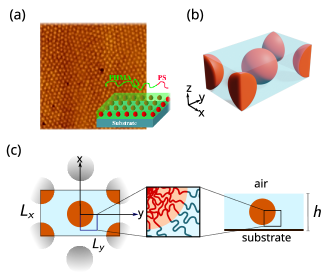
Experiment. The PS-PHMA diblock employed here was synthesized via sequential living anionic polymerization of styrene and n-hexyl methacrylate, in tetrahydrofuran at -78∘C, using 10 eq of LiCl to s-butyllithium initiator. The sphere-forming diblock had block molar masses of 18 and 95 kg/mol (see refs. 26, 10, 27 for more details ). A monolayer of diblock copolymer was made by spin-coating a solution of PS-PHMA in toluene ( 1 wt. ) onto silicon wafer (SiliconQuest, with native oxide). The thickness of the film was controlled through the spin speed. The silicon wafer was pre-washed at least five times with toluene and dried under flowing nitrogen prior to use. The polymer film thickness was measured using a PHE101 ellipsometer (Angstrom Advanced Inc.; wavelength = 632.8 nm). The morphology was characterized at room temperature using atomic force microscopy (Innova, Bruker) operated in tapping mode using uncoated silicon tips having a cantilever length of 125 m, spring constant of 40 N/m, and resonant frequency of 60 90 kHz, purchased from NanoWorld. Since the PS spheres are glassy and the PHMA matrix rubbery at room temperature, AFM phase imaging of the films reveals the underlying structure and the local order developed by the block copolymer. To improve the image quality, the micrograph was flattened and filtered by performing a discrete Fourier transform to remove high and low frequency noise. Fig. 1a shows the pattern developed by the arrays of PS spheres after 12 hours of thermal annealing at 125 ∘C. Thin films thickness 35 nm.
SCF calculations. We consider a melt of coarse-grained, flexible AB diblock copolymer molecules with a degree of polymerization , symmetric segment length , and a volume fraction for the A-block. The interactions between the polymer chains are characterized by the dimensionless incompatibility parameter and compressibility parameter . We consider symmetric films, corresponding to a situation where the surface interactions on both sides of the films are identical, both showing a preference for A-blocks. The SCFT calculations are conducted in a periodic cuboid cell with a volume of (Fig. 1b-c) in the grand canonical ensemble, i.e., a fixed chemical potential of the copolymer melt is used. More details can be found in Supplementary Information S1.
We first obtain the stable sphere structure by minimizing the free energy per unit area of the melt, , with respect to the transverse periodicity of the sphere domains () and cell thickness (). The transverse cell shape in this case is fixed to , corresponding to a hexagonal pattern. We will see below that this indeed corresponds to the energetically preferred shape. In our calculation, the chemical potential of the copolymer melt is fixed to , where is the dimensionless Ginzburg parameter, is the average monomer density, and is the radius of gyration of one polymer chain. The modified diffusion equation is solved in real space using the Crank-Nicolson scheme and the alternative direction implicit (ADI) method (numerical details can be found in Supplementary Information S3). We use a contour discretization of and a spatial discretization using a grid system of . A finer discretization is chosen in the direction to minimize the discretization error arising from the external surface interaction potential applied at the interface.
3 Results and discussion
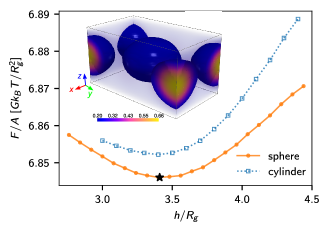
Previous SCFT calculations predict that the sphere phase exists in a very narrow window ( for ) in the bulk phase diagram of AB diblock-copolymers 21. Here we choose , , and . For this value of the compressibility parameter, the density inside the film is the same for all simulations within 0.03%. The strength of surface interaction between surface and copolymer blocks A and B per surface area is and , in units . Fig. 2 shows the SCFT results for the free energy per area as a function of the film thickness . In an SCFT study of a similar system, Li et al. obtained a transition from sphere (at small ) to cylindrical (at larger ) around 25. Our SCFT calculations, instead, predict a stable sphere phase for film thickness . We attribute this difference to the varied asymmetries in the surface interactions with A- and B-blocks, a factor we found to be critical in constructing the phase diagram of thin films. We have tested that the free energy of the (metastable) cylinder phase (blue dotted curve in Fig. 2) is indeed higher than that of the other phases with our choice of parameters. The optimal lateral inter-sphere spacing in our system is found to be and the optimum thickness is , corresponding to an incommensurability parameter of . This is in reasonably good agreement with our experimental result, . Matching the periodicity and the film thickness to the experiments, we can estimate , and thus , by assuming an average copolymer density of at room temperature 28.
To calculate the elastic constants, we analyze the free energy response of the system to small perturbations of the size or shape of the cell used in the SCFT calulations (Fig. 1b). In the linear regime, the general form of the resulting free energy change should take the form , where is the rank-four elastic modulus tensor, and is the strain tensor (). Since only in-plane extension/compression and shearing are considered, the elastic free energy for the BCP film can generally be decomposed as 29
| (1) |
where , , and are the extensional moduli and is the shear modulus. For simplicity purposes, we use the Voigt notations for the moduli, where the the subscripts 1, 2 and 6 correspond to , and . We calculate the elastic moduli by numerically evaluating the variation in the SCFT free energy of the BCP film after a small deformation, such that the film can still re-equilibrate. The second derivative of the free energy with respect to strain gives the elastic moduli. We impose seven different types of in-plane deformations to the film by varying cell size and shape as follows as shown in Fig. 3a. Table 1 summarizes different types of deformations and their associated strain components and the combined elastic moduli that contribute to the free energy change. The calculated free energy difference, , after deformation can be fitted with a parabolic function, , where is the relative deformation and is effective modulus for deformations type . We derive the effective elastic moduli, for each individual deformation from eq. 1. By fitting the SCFT data in Fig. 3b for all seven deformations collectively, we obtain the elastic modulus , , and . Each deformation also induces a small change in the film thickness, shown in Fig. 3b. Figure 3a shows the different types of deformations and the changes in free energy as a function of relative deformations.
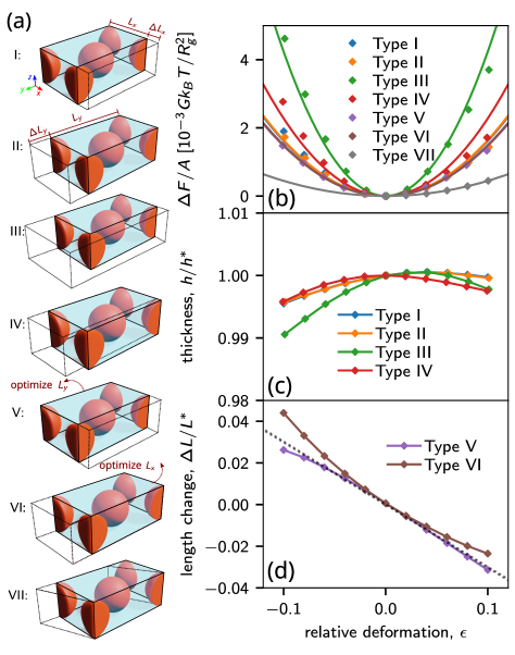
| Type | strain | ||
| I | |||
| II | |||
| III | |||
| IV | , | ||
| V | , | ||
| VI | , | ||
| VII | |||
For two-dimensional structures with six-fold or four-fold symmetry, one expects the elastic energy (1) to take the form 29
| (2) |
where is the compression modulus and , are the pure shear and the simple shear modulus, respectively. This implies , , and . In systems with hexagonal symmetry, one additionally expects the pure shear and the simple shear modulus to be identical, . Our results indeed confirm the relation within the error. However, the pure shear modulus, , differs from the simple shear modulus, . We attribute this unexpected discrepancy to nonlinear higher-order effects, which apparently influence the effective elastic constants already at small deformations. Nevertheless, since , the film still retains the characteristics of a square symmetry, which explains why shear-aligning such films is so difficult. The Poisson ratios along the x-axis and y-axis are given by and , which is consistent with Figure 3d.
Next we study the coupling between BCP films and curvature. To this end, we consider films that are confined between two coaxial cylinders with a middle-surface curvature of , as shown in the inset of Fig. 4. The bending free energy per unit area of an isotropic fluid-like membrane can be described by the Helfrich formula 30, 31: , where is the bending modulus, is the Gaussian (or saddle-splay) modulus for saddle-like deformations, , and are the mean, spontaneous, and Gaussian curvatures, respectively, while and are the principal curvatures. For cylindrical bending, we simply have , where is the corresponding curvature of the middle surface of the membranes, and the Gaussian saddle-like deformation vanishes, . Since we consider films with symmetric surface interactions, the spontaneous curvature vanishes as well, i.e., . Therefore, the overall bending free energy is simply a quadratic function of the curvature, with the bending constant .
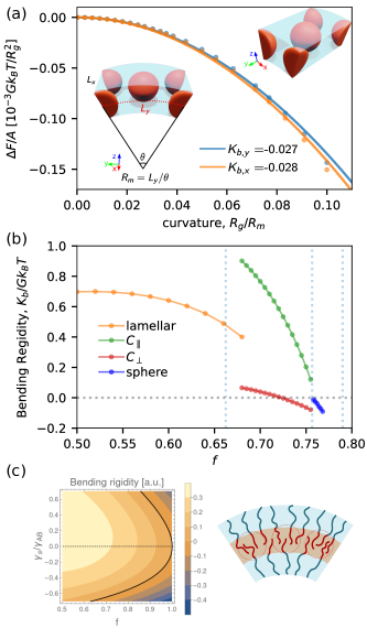
The SCFT calculations are done in cylindrical coordinates. The resulting free energy change per surface area is shown as a function of the curvature radius in Fig. 4 a. Surprisingly, the free energy decreases if the film is bent: A quadratic fit to the concave energy curves give two “negative” bending constants. This implies that free-standing symmetric sphere-patterned monolayer films are inherently unstable, according to the SCFT predictions, different from the cylindrically patterned monolayers which we studied previously 12. The two bending constants and for bending in the and directions are very close to each other, making it very unlikely that curvature could be used for pattern orientation. The BCP films show a very slight tendency of bending in the direction of the -axis, which is also the direction of nearest neighbors. We should note that the absolute value of is much smaller for sphere-patterned BCP films than for cylinder-forming films. Nevertheless, the change of sign leads to a fundamentally different qualitative behavior of the films.
To investigate the origin of this behavior, we have calculated the bending rigidities for a large range of block fractions , see Fig. 4b). As a function of , the BCP film undergoes a sequence of structural phase transitions from lamellar to cylinders (C) to sphere. The bending rigidity jumps at phase boundaries, but apart from these discontinuities, it generally decreases with increasing . We speculate that, as the copolymer becomes more asymmetric, the individual chains, under bending, tend to rearrange themselves to minimize the interfacial energies and the chain entropy. Strong stretching theory (SST) calculations32, 33, 34 for the lamellar structures (for derivations and equations see Supporting information S2) show that this indeed leads to a decrease of the bending constant and enables negative bending constants at large , see Fig. 4c.
4 Conclusions
In conclusion, we have determined the in-plane elastic moduli and the orientation dependent bending moduli of thin symmetric sphere-patterned films. Our results show that the film shows nearly isotropic behavior, and in particular, the coupling between curvature and in-plane structure is much weaker than in cylinder-forming BCP films. This explains the experimental observation that shear-alignment of sphere monolayer films seems almost impossible, and suggests that curvature-based alignment strategies will also not be successful. Most importantly, the calculations predict that the bending moduli of sphere monolayers are negative. This implies that a free-standing single-layered BCP film in the sphere phase should inherently be unstable towards bending, potentially explaining experimental challenges (see below) in achieving either curved crystal monolayers or stable free-standing monolayers at temperatures above the glass transition temperature of both blocks.
We have explored two different sphere forming block copolymers to obtain monolayers of free-standing membranes: poly(styrene)-block-poly(ethylene-alt-propylene) and poly(styrene)-block- poly(n-hexylmethacrylate). In both cases, we found that the free standing films become unstable upon increasing the temperature well above 100, transitioning the diblock copolymer into a molten state. In addition, we have also explored the stability of a monolayer of sphere forming PE-PEP block copolymer deposited via spin casting onto a curved substrate. While in this case, polymer-substrate and polymer-air interfaces has different surface energies, we found that the polymer film becomes unstable and dewets even at regions with shallow curvatures.
However, it’s important to note that Mansky et al.35 demonstrated that free-standing sphere-forming diblock copolymer films could be achieved using polystyrene-block-polybutadiene diblocks with a spherical microstructure. This implies that film stability may not be universally predetermined and could vary based on factors such as surface tension, TEM grid size, TEM grid-polymer interactions, and the stress-strain fields introduced during sample preparation. In order to stabilize self-assembled sphere-patterned monolayer films, special strategies will have to be applied, such as, early crosslinking36 , employing high molecular weight triblock copolymers or using selective and temperature-tunable solvent37, 38. Alternatively, it may be possible to obtain stable films from melts where the close-packed cubic phases have a wider range of stability, e.g., due to additives 39, 40, 41 or due to the effect of polydispersity of the different blocks 42, 43, 44.
This work was funded by the Deutsche Forschungsgemeinschaft (DFG, Germany), Grant number 248882694. We also gratefully acknowledge financial support from the Deutsche Froschungsgemeinschaft – SFB 1552, Grant Number 465145163, Project C01, from the National Science Foundation MRSEC Program through the Princeton Center for Complex Materials (DMR-1420541), Universidad Nacional del Sur, and the National Research Council of Argentina (CONICET). We thank Richard Register for providing us the diblock copolymer.
5 S1: Self-consistent field Theory (SCFT)
Self-consistent field theory has proven to be a powerful approach for describing and predicting equilibrium structures in inhomogeneous polymer systems. In this study, we consider a melt of asymmetric AB diblock copolymer molecules with a degree of polymerization , confined between two flat (coaxial cylindrical) surfaces separated by a distance of h. We assume that the majority block A takes a fraction of each diblock copolymer chain, and both blocks share the same monomer size . The microscopic concentration operators of A and B segments at a given point are given by:
| (3) | |||
| (4) |
where is the average copolymer density, is the total number of copolymer molecules and is the volume of the film. Here and throughout, we will set . The interaction potential of the melt is thus
| (5) |
where is the Flory-Huggins parameter specifying the repulsion of and segments. is the inverse of isothermal compressibility parameter and are surface energy fields. We assume that symmetric boundary wetting conditions, the surfaces interact energy with A and B segments are and , respectively. We choose a surface field of width , given by
| (6) |
In our model, we choose and is the radius of gyration of one polymer chain. In the grand canonical ensemble, the free energy has the form
| (7) |
where is chemical potential, is the partition function of a single non-interacting polymer chain,
| (8) |
and end-segment distribution functions and satisfy the modified diffusion equation
| (9) |
with
| (10) |
and the initial condition . The diffusion equation for is similar with replaced by and the same initial condition, . By finding the extremum of the free energy with respect to and , we get the self-consistent equations,
| (11) | ||||
| (12) | ||||
| (13) | ||||
| (14) |
6 S2: Strong-stretching theory (SST)
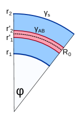
In the SST calculations, we consider the cylindrical geometry sketched in Fig. 5, and, for completeness, the corresponding spherical geometry. Two copolymer layers (labeled ) face each other at the radius . The two outer surfaces of the film are found at the radii and . The thickness of the film is thus , and the bilayer midplane is located at . Our goal is to minimize the grand canonical free energy per area as a function of with respect to and and expand it in powers of . This will allow us to calculate the bending rigidity and the Gaussian rigidity in the free energy expression.
| (15) |
for a general curved surface with total curvature and Gaussian curvature (the are the principal curvatures).
To proceed, we first calculate the canonical (Helmholtz) free energy. In SST approximation, it is given as the sum of the interfacial energies and stretching energies in the system47. The interfacial energy per area at the radius is given
where is the surface free energy per area of the film and the interfacial free energy between A and B domains ( in the Strong-stretching limit).
The total stretching energy in SST approximation can be calculated from 47
with . Since the copolymers are incompressible, the ratio of volumes and occupied by A monomers and all monomers is . This results in the cylindrical case in the constraints for , and in the spherical case . To account for them, we introduce the variable and , which is roughly (not exactly) the thickness of the monolayer . In terms of , taking into account the constraints, the radii , can be written as
with in the cylindrical case and in the spherical case. We insert these expressions in the above equations for the free energy and expand the result in powers of , which is a small parameter for weakly bent membranes. The result has the form
with the coefficients
| (16) |
The contact radius may deviate from the mid radius of the bilayer, , the reference plane for the definition of the bending rigidity. Therefore, in the next step, we rewrite the total free energy per area at the mid radius as an expansion in powers of , for given total thickness , and minimize it with respect to . To this end, we define a set of reduced quantities, (the new small parameter), (accounting for the fact that as ), and . Using these quantities, minimizing with respect to at fixed , and keeping only terms up to order , we get
| (17) |
with
| (18) | |||||
| (19) |
in the cylindrical and spherical geometry, respectively. From these two results, we can calculate the bending rigidity and the Gaussian rigidity for films of fixed thickness via and . The result is
| (20) | |||||
| (21) |
Finally, we switch to the grand canonical ensemble and minimize the grand canonical free energy
| (22) |
with respect to . Here is the chemical potential, is the monomer density, and is the film volume per area . We consider a general curved geometry with total curvature and mean curvature , assuming that both are small, i.e., and with . The general expression for the Helmholtz free energy per area of a film with given thickness is given by
| (23) |
The volume per area can be calculated from
| (24) |
We minimize with respect to and expand again in powers of the small parameter, . In the planar case, the minimization gives
| (25) |
and the corresponding planar free energy is
| (26) |
In curved films, the optimal thickness deviates from by an amount which is proportional to , . Since is a minimum with respect to , this correction only contributes to quadratic order, hence order , to , and can be neglected. Thus we obtain
| (27) |
Following Ajdari and Leibler33, we now consider specifically the chemical potential where the planar film just becomes stable, i.e., , which implies
| (28) |
(with the statistical segment length ). The latter expression is also given in Ref. 33 for . At this value of , the thickness and in particular the reduced parameter take the simple form
| (29) |
Inserting this in the equations for and , we finally obtain the following expressions for the bending rigidity and the effective Gaussian rigidity:
| (30) | |||||
| (31) |
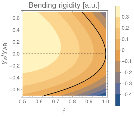
in the free energy expansion (15) (at ). In the special case , these equations reproduce the result of Ajdari and Leibler33 (taking into account that these authors define as in our notation). Inspecting the free energy expression (15) reveals two stability conditions for a flat bilayer: and . Figure 6 shows the rescaled results for and as a function of and , also indicating this stability region. The rescaling constant is .

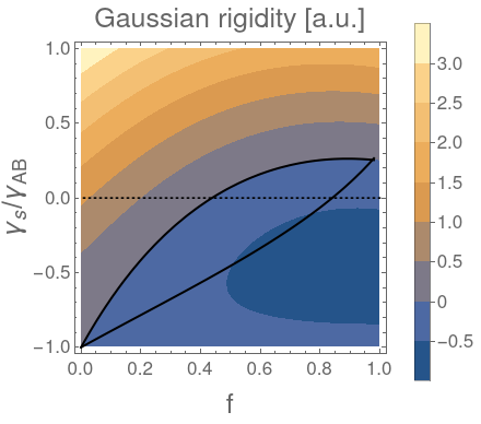
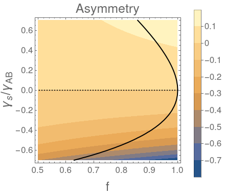
In the lamellar state, for , the bending rigidity generally decreases with , and eventually becomes negative for all values of surface tension except . To rationalize this behavior, it is instructive to investigate the asymmetry of the bent film in the cylindrical geometry, i.e., the extent to which the contact surface between the monolayers, located at , deviates from the mid surface of the bilayer, . We define the asymmetry parameter via (recalling ). Its value is obtained as
| (32) |
and shown in Figure 7(right). The asymmetry of the film results from two opposing driving factors: At fixed , the interfacial energy due to AB incompatibility () can be reduced if is driven inwards, towards smaller values, because this reduces the total AB interfacial area. (At constant , the total outer surface area is constant in the cylindrical geometry). On the other hand, the stretching energy benefits if is driven outwards: Single copolymers in the inner monolayer are more stretched (lose energy), whereas single copolymers in the outer monolayer are less stretched (gain energy). Since the outer layer contains more copolymers, the net effect is positive for . This latter factors dominates if the film thickness is large, i.e., is large. Then we find . If is small, i.e., is small, the effect of the interfacial energy dominates, and we find . It is interesting to note that the two effects exactly compensate each other in the case . In that case, and the bending rigidity is always positive.
Finally, we note that instead of minimizing the grand canonical free energy per area with respect to the film thickness , we could also minimize the canonical Helmholtz free energy per chain, i.e., per volume. In the planar case, this results in the same optimal thickness (Eq. (29)) than before, and the Helmholtz free per chain reads
| (33) |
where and are given by Eqs. (30), (31). Hence the results from the two approaches are consistent.
7 S3: Numerical Details of ADI Method
The SCFT calculations are done in Cartesian and Cylindrical coordinates with Dirichlet boundary conditions in the direction normal to the surface and periodic boundary conditions in two in-plane directions. The modified diffusion equation is solved numerically using the Crank-Nicolson scheme and alternative direction implicit (ADI) method.
7.1 3D ADI Algorithm: Cartesian Coordinate
The three dimensional diffusion equation of the propagator in Cartesian coordinate has the form
| (34) |
In order to solve eq. 34, we apply the Crank-Nicolson scheme in using Douglas-Gunn ADI scheme by introducing two intermediate variables and . The discretization of eq. 34 is done by splitting into three subset of equations:
| (35) | ||||
| (36) | ||||
| (37) |
where denotes the grid points in -direction, denotes the grid points in the -direction, and denotes the grid points in the -direction. , , and are interval sizes in space. Using the second-order central difference algorithm, the second derivative with respect to can be approximated as
| (38) |
Approximate and rearrange above equations, we obtain the three-step ADI
| (39) |
| (40) |
| (41) |
7.2 3D ADI: Cylindrical coordinates
The modified diffusion equation in three Dimensional Cylindrical Coordinates reads;
| (42) |
Applying the ADI method to the CN scheme, we split the calculation into 3 sub-steps to implicitly solve eq. 42 in , and directions at step , and , The discretization of eq. 42 gives
| (43) | ||||
| (44) | ||||
| (45) | ||||
where , , and , are the grid points in , and directions, respectively. Again using the second-order central difference algorithm, the operator is simply,
| (46) | |||
| (47) |
Combining and rearranging eqs. 43-45, we have
| (48) | |||
| (49) | |||
| (50) | |||
7.3 Shear transformation: Cartesian Coordinates
To find the shear elasticity of the monolayer film, we do a simple shear transformation of the Laplacian by applying the Laplace-Beltrami operator to eq. 34
| (51) |
where is the metric tensor and is its inverse. The shear transformation to the orthogonal coordinate in matrix form is
| (52) |
where and is the shear angle in x-direction. The metric tensor is thus given by
| (53) |
Here the determinant of the Jacobian and the metric tensor are and respectively, and the inverse is given by
| (54) |
The transformed Laplacian is thus
| (55) |
7.3.1 Splitting scheme
In the presence of the mixed derivative term in eq. 55, we use the splitting scheme proposed by Hundsdorfer 45, 46, which solves explicitly and the rest implicitly.
| (56) |
The fourth-order approximation of the mixed derivative term is simply
| (57) | ||||
| (58) |
where denotes a real parameter with . The right-hand side is the most general form of a second-order approximation for the cross derivative based on a centered 9-point stencil. When reduces to the standard 4-point stencil
| (59) |
References
- Yang et al. 2022 Yang, G. G.; Choi, H. J.; Han, K. H.; Kim, J. H.; Lee, C. W.; Jung, E. I.; Jin, H. M.; Kim, S. O. Block Copolymer Nanopatterning for Nonsemiconductor Device Applications. ACS Appl. Mater. Interfaces 2022, 14, 12011–12037
- Karayianni and Pispas 2021 Karayianni, M.; Pispas, S. Block Copolymer Solution Self-Assembly: Recent Advances, Emerging Trends, and Applications. J. Polym. Sci. 2021, 59, 1874–1898
- Kulkarni and Doerk 2022 Kulkarni, A. A.; Doerk, G. S. Thin Film Block Copolymer Self-Assembly for Nanophotonics. Nanotechnology 2022, 33, 292001
- Huang et al. 2021 Huang, C.; Zhu, Y.; Man, X. Block Copolymer Thin Films. Phys. Rep. 2021, 932, 1–36
- Albert and Epps 2010 Albert, J. N. L.; Epps, T. H. Self-Assembly of Block Copolymer Thin Films. Mater. Today 2010, 13, 24–33
- Li and Müller 2015 Li, W.; Müller, M. Defects in the Self-Assembly of Block Copolymers and Their Relevance for Directed Self-Assembly. Annu. Rev. Chem. Biomol. Eng. 2015, 6, 187–216
- García et al. 2015 García, N. A.; Pezzutti, A. D.; Register, R. A.; Vega, D. A.; Gómez, L. R. Defect Formation and Coarsening in Hexagonal 2D Curved Crystals. Soft Matter 2015, 11, 898–907
- Morkved et al. 1996 Morkved, T. L.; Lu, M.; Urbas, A. M.; Ehrichs, E. E.; Jaeger, H. M.; Mansky, P.; Russell, T. P. Local Control of Microdomain Orientation in Diblock Copolymer Thin Films with Electric Fields. Science 1996, 273, 931–933
- Marencic et al. 2007 Marencic, A. P.; Wu, M. W.; Register, R. A.; Chaikin, P. M. Orientational Order in Sphere-Forming Block Copolymer Thin Films Aligned under Shear. Macromolecules 2007, 40, 7299–7305
- Kwon et al. 2014 Kwon, H.-K.; Lopez, V. E.; Davis, R. L.; Kim, S. Y.; Burns, A. B.; Register, R. A. Polystyrene-poly(2-ethylhexylmethacrylate) block copolymers: Synthesis, bulk phase behavior, and thin film structure. Polymer 2014, 55, 2059–2067
- Nowak and Yager 2020 Nowak, S. R.; Yager, K. G. Photothermally Directed Assembly of Block Copolymers. Adv. Mater. Interfaces 2020, 7, 1901679
- Vu et al. 2018 Vu, G. T.; Abate, A. A.; Gómez, L. R.; Pezzutti, A. D.; Register, R. A.; Vega, D. A.; Schmid, F. Curvature as a Guiding Field for Patterns in Thin Block Copolymer Films. Phys. Rev. Lett. 2018, 121, 087801
- Kossuth et al. 1999 Kossuth, M. B.; Morse, D. C.; Bates, F. S. Viscoelastic Behavior of Cubic Phases in Block Copolymer Melts. J. Rheol. 1999, 43, 167–196
- Tyler and Morse 2003 Tyler, C. A.; Morse, D. C. Linear Elasticity of Cubic Phases in Block Copolymer Melts by Self-Consistent Field Theory. Macromolecules 2003, 36, 3764–3774
- Thompson et al. 2004 Thompson, R. B.; Rasmussen, K. O.; Lookman, T. Elastic Moduli of Multiblock Copolymers in the Lamellar Phase. J. Chem. Phys. 2004, 120, 3990–3996
- Li et al. 2013 Li, J.; Pastor, K. A.; Shi, A.-C.; Schmid, F.; Zhou, J. Elastic Properties and Line Tension of Self-Assembled Bilayer Membranes. Phys. Rev. E 2013, 88, 012718
- Bates and Fredrickson 1999 Bates, F. S.; Fredrickson, G. H. Block Copolymers—Designer Soft Materials. Phys. Today 1999, 52, 32–38
- Saito et al. 2022 Saito, M.; Ito, K.; Yokoyama, H. Film Thickness and Strain Rate Dependences of the Mechanical Properties of Polystyrene-b-Polyisoprene-b-Polystyrene Block Copolymer Ultrathin Films Forming a Spherical Domain. Polymer 2022, 258, 125302
- Marencic et al. 2010 Marencic, A. P.; Adamson, D. H.; Chaikin, P. M.; Register, R. A. Shear Alignment and Realignment of Sphere-Forming and Cylinder-Forming Block-Copolymer Thin Films. Phys. Rev. E 2010, 81, 011503
- Angelescu et al. 2005 Angelescu, D. E.; Waller, J. H.; Register, R. A.; Chaikin, P. M. Shear-Induced Alignment in Thin Films of Spherical Nanodomains. Adv. Mater. 2005, 17, 1878–1881
- Matsen 2009 Matsen, M. W. Fast and Accurate SCFT Calculations for Periodic Block-Copolymer Morphologies Using the Spectral Method with Anderson Mixing. Eur. Phys. J. E 2009, 30, 361
- Geisinger et al. 1999 Geisinger, T.; Müller, M.; Binder, K. Symmetric Diblock Copolymers in Thin Films. I. Phase Stability in Self-consistent Field Calculations and Monte Carlo Simulations. J. Chem. Phys. 1999, 111, 5241–5250
- Hur et al. 2009 Hur, S.-M.; García-Cervera, C. J.; Kramer, E. J.; Fredrickson, G. H. SCFT Simulations of Thin Film Blends of Block Copolymer and Homopolymer Laterally Confined in a Square Well. Macromolecules 2009, 42, 5861–5872
- Mishra et al. 2011 Mishra, V.; Fredrickson, G. H.; Kramer, E. J. SCFT Simulations of an Order–Order Transition in Thin Films of Diblock and Triblock Copolymers. Macromolecules 2011, 44, 5473–5480
- Li et al. 2013 Li, W.; Liu, M.; Qiu, F.; Shi, A.-C. Phase Diagram of Diblock Copolymers Confined in Thin Films. J. Phys. Chem. B 2013, 117, 5280–5288
- Varshney et al. 1990 Varshney, S. K.; Hautekeer, J.; Fayt, R.; Jérôme, R.; Teyssié, P. Anionic polymerization of (meth) acrylic monomers. 4. Effect of lithium salts as ligands on the” living” polymerization of methyl methacrylate using monofunctional initiators. Macromolecules 1990, 23, 2618–2622
- García et al. 2014 García, N. A.; Davis, R. L.; Kim, S. Y.; Chaikin, P. M.; Register, R. A.; Vega, D. A. Mixed-morphology and mixed-orientation block copolymer bilayers. RSC Adv. 2014, 4, 38412–38417
- Kim et al. 2014 Kim, S. Y.; Nunns, A.; Gwyther, J.; Davis, R. L.; Manners, I.; Chaikin, P. M.; Register, R. A. Large-Area Nanosquare Arrays from Shear-Aligned Block Copolymer Thin Films. Nano Lett. 2014, 14, 5698–5705
- Boal 2002 Boal, D. Mechanics of the Cell; Cambridge University P: Cambridge, 2002
- Helfrich 1973 Helfrich, W. Elastic Properties of Lipid Bilayers: Theory and Possible Experiments. Z. Naturforsch. C 1973, 28, 693–703
- Safran 1999 Safran, S. A. Curvature Elasticity of Thin Films. Adv. Phys. 1999, 48, 395–448
- Milner and Witten 1988 Milner, S.; Witten, T. Bending Moduli of Polymeric Surfactant Interfaces. J. de Physique 1988, 49, 1951–1962
- Ajdari and Leibler 1991 Ajdari, A.; Leibler, L. Bending Moduli and Stability of Copolymer Bilayers. Macromolecules 1991, 24, 6803–6804
- Wang 1992 Wang, Z. Curvature Instability of Diblock Copolymer Bilayers. Macromolecules 1992, 25, 3702–3705
- Mansky et al. 1995 Mansky, P.; haikin, P.; Thomas, E. L. Monolayer Films of Diblock Copolymer Microdomains for Nanolithographic Applications. J. Mater. Sci. 1995, 30, 1987–1992
- Quémener et al. 2010 Quémener, D.; Bonniol, G.; Phan, T. N. T.; Gigmes, D.; Bertin, D.; Deratani, A. Free-Standing Nanomaterials from Block Copolymer Self-Assembly. Macromolecules 2010, 43, 5060–5065
- Sohn et al. 2001 Sohn, B.-H.; Yoo, S.-I.; Seo, B.-W.; Yun, S.-H.; Park, S.-M. Nanopatterns by Free-Standing Monolayer Films of Diblock Copolymer Micelles with in Situ Core-Corona Inversion. J. Am. Chem. Soc. 2001, 123, 12734–12735
- Lu et al. 2010 Lu, H.; Lee, D. H.; Russell, T. P. Temperature Tunable Micellization of Polystyrene- Block -Poly(2-Vinylpyridine) at Si-Ionic Liquid Interface. Langmuir 2010, 26, 17126–17132
- Matsen 1995 Matsen, M. W. Stabilizing New Morphologies by Blending Homopolymer with Block Copolymer. Phys. Rev. Lett. 1995, 74, 4225
- Huang et al. 2003 Huang, Y.-Y.; Chen, H.-L.; Hashimoto, T. Face-centered Cubic Lattice of Spherical Micelles in Block Copolymer-homopolymer Blends. Macromolecules 2003, 36, 764–770
- Chen et al. 2019 Chen, L.-T.; Chen, C.-Y.; Chen, H.-L. FCC or HCP: The Stable Close-packed Lattice of Crystallographically Equivalent Spherical Micelles in Block copolymer/homopolymer Blends. Polymer 2019, 169, 131–137
- Matsen 2007 Matsen, M. W. Polydispersity-induced Macrophase Separation in Diblock copolymer melts. Phys. Rev. Lett. 2007, 99, 148304
- Matsen 2013 Matsen, M. W. Comparison of A-block Polydispersity Effects on BAB Triblock and B Diblock Copolymer Melts. Eur. Phys. J. E 2013, 36, 44
- Zhang et al. 2021 Zhang, C.; Vigil, D. L.; Sun, D.; Bates, M. W.; Loman, T.; Murphy, E. A.; Barbon, S. M.; Song, J.-A.; Yu, B.; Fredrickson, G. H.; Whittaker, A. K.; Hawker, C. J.; Bates, C. M. Emergence of Hexagonally Close-Packed Spheres in Linear Block Copolymer Melts. J. Am. Chem. Soc. 2021, 143, 14106–14114
- Hundsdorfer 2002 Hundsdorfer, W. Accuracy and Stability of Splitting with Stabilizing Corrections. Appl. Numer. Math. 2002, 42, 213–233
- in ’t Hout and Welfert 2007 in ’t Hout, K. J.; Welfert, B. D. Stability of ADI Schemes Applied to Convection–Diffusion Equations with Mixed Derivative Terms. Appl. Numer. Math. 2007, 57, 19–35
- Matsen 2001 Matsen, M. W. The Standard Gaussian Model for Block Copolymer Melts. J. Phys.: Cond. Matter 2001, 14, R21