An Arbitrarily High-Order Fully Well-balanced Hybrid Finite Element-Finite Volume Method for a One-dimensional Blood Flow Model

Abstract

In this paper, we propose an arbitrarily high-order accurate fully well-balanced numerical method for the one-dimensional blood flow model. The developed method is based on a continuous representation of the solution and a natural combination of the conservative and primitive formulations of the studied PDEs. The degrees of freedom are defined as point values at cell interfaces and moments of the conservative variables inside the cell, drawing inspiration from the discontinuous Galerkin method. The well-balanced property, in the sense of an exact preservation of both the zero and non-zero velocity equilibria, is achieved by a well-balanced approximation of the source term in the conservative formulation and a well-balanced residual computation in the primitive formulation. To lowest (3rd) order this method reduces to the method developed in [Abgrall and Liu, A New Approach for Designing Well-Balanced Schemes for the Shallow Water Equations: A Combination of Conservative and Primitive Formulations, arXiv preprint, arXiv:2304.07809]. Several numerical tests are shown to prove its well-balanced and high-order accuracy properties.

Key words: Blood flows, Well-balanced schemes, Arbitrarily high-order methods, Moments of conservative variables, Finite element-Finite volume method

AMS subject classification: 35L60, 65M08, 65M60, 76M10, 76M12

1 Introduction

One-dimensional (1-D) blood flow models have proven to be valuable tools for mathematically understanding and numerically addressing fundamental aspects of pulse wave propagation in the human cardiovascular system; see, e.g., [38, 5, 39]. 1-D models with averaged quantities are simpler, and they are also useful in numerical simulation of blood flow, as shown in [46, 47]. One key advantage of 1-D models is their lower computational cost, which allows for the study of wave effects in isolated arterial segments or systemic arterial systems (i.e. in the aorta and systemic arteries) [37, 41, 42, 45]. Furthermore, 1-D models can be easily coupled with lumped-parameter models [44, 47] and three-dimensional fluid-structure models [24, 25, 43, 9, 8], making them a powerful tool for constructing comprehensive models of the human cardiovascular system.

A well-established partial differential equation (PDE) model for the 1-D blood flow through human arteries takes the form (see, e.g., [10], the review paper [48] and references therein):

$$\left\{\begin{aligned} &A_{t}+Q_{x}=0,\\ &Q_{t}+\Big{(}\widehat{\alpha}\frac{Q^{2}}{A}\Big{)}_{x}+\frac{A}{\rho}p_{x}=0,\end{aligned}\right.$$ (1.1)

where $A(x,t)=\pi R^{2}(x,t)$ is the cross-sectional area of the vessel with $R(x,t)>0$ being the radius and $Q(x,t)=A(x,t)u(x,t)$ is the discharge with $u(x,t)$ being the averaged velocity of blood at a cross section. $\rho$ represents the fluid density which is assumed to be constant and $p(x,t)$ denotes the averaged internal pressure which will be given later to close the description of the system (1.1). The parameter $\widehat{\alpha}$ is the momentum-flux correction coefficient that depends on the assumed velocity profile. For simplicity, in this paper we take $\widehat{\alpha}\equiv 1$, which corresponds to a blunt velocity profile.

Note that there are more unknowns than equations in (1.1) and hence a closure condition linking the pressure with the displacement of the vessel will be needed. From mechanical consideration, in the present work, a simple tube law describing the elastic behaviour of the arterial wall is given by

$$p(x,t)=p_{\rm ext}+\frac{\kappa}{\sqrt{\pi}}\Big{(}\sqrt{A(x,t)}-\sqrt{A_{0}(x)}\Big{)},$$ (1.2)

where $p_{\rm ext}$ is the external pressure and assumed to be constant, the constant parameter $\kappa$ stands for arterial stiffness, and $A_{0}(x)=\pi(R_{0}(x))^{2}$ is the cross-section at rest (when $u=0$) with $R_{0}(x)$ being its radius. Using the usual tube law (1.2), we can rewrite the 1-D blood flow model (1.1) in the form of hyperbolic balance laws:

$$\left\{\begin{aligned} &A_{t}+Q_{x}=0,\\ &Q_{t}+\Big{(}\frac{Q^{2}}{A}+\frac{\beta}{3}A^{\frac{3}{2}}\Big{)}_{x}=\frac{\beta A}{2\sqrt{A_{0}}}(A_{0})_{x},\end{aligned}\right.$$ (1.3)

where $\beta=\frac{\kappa}{\rho\sqrt{\pi}}$. For details, we refer to the review paper [48] and references therein. In Figure 1.1, we present a 1-D blood flow model diagram with the cross-sectional radius $(R)$, the radius at rest $(R_{0})$, and velocity $(u)$.

Figure 1.1: Diagram (also see [10, Figure 1]) of the 1-D blood flow model with the cross-sectional radius ($R$), the radius at rest ($R_{0}$), and velocity $u$.

The momentum balance equation in (1.3) contains source terms that rely on the spatial derivatives of tube law parameters. These terms, also known as geometric source terms, are similar to those present in shallow water equations with non-flat bottom topography,as can be seen in references, e.g., [32, 18, 15, 33, 17, 51]. Both the shallow water equations and the blood flow system (1.3) belong to the family of hyperbolic balance laws, which often have non-trivial steady-state solutions. These solutions respect a delicate balance between the flux gradients and the source terms of the studied system at PDE level. In practical simulations with affordable mesh refinement, a good numerical method is required to exactly preserve the perfect cancellation of the flux gradients and the source terms at the discrete level as well as accurately capture the nearly equilibrium flow. Such method is often referred to as a well-balanced (WB) method.

Various WB numerical methods have been developed for the 1-D shallow water equations; see, e.g., [12, 13, 14, 16, 15, 17, 29, 36, 51, 11]. These methods usually involve either a non-trivial root-finding mechanism based on energy balance, or significant effort in local reconstruction of the conservative variables or complex reconstruction of the geometric source terms. In a recent work [32], the authors proposed a partial relaxation scheme to preserve moving-water equilibria of the shallow water equations, which avoids the aforementioned complexities at least for flows that are in the subcritical regime. It is worth mentioning that a very recent study [4] developed a new approach for designing a fully WB scheme of the shallow water equations that can overcome the complexities mentioned above for any flow. The key idea of this new approach is to work with both the conservative and primitive formulations of the studied PDE and develop a combined method in a WB manner.

The literature on well-balanced schemes for modeling 1-D blood flow through arteries is extensive, with numerous methods having been thoroughly studied over the past decade. For instance, in [21], WB first- and second-order finite volume schemes were developed to exactly preserve the zero-velocity stationary solutions. In [34], an Arbitrary high-order DERivatives (ADER) finite volume framework was utilized to construct a WB numerical scheme for 1-D blood flow in elastic vessels with varying mechanical properties. In [50], high-order WB finite difference weighted essentially non-oscillatory (WENO) schemes for the blood flow model were derived based on a specific splitting of the source term into two parts, which were then discretized separately with compatible WENO operators. Additionally, in [31], the hydrostatic reconstruction was used to construct high-order discontinuous Galerkin (DG) and finite volume WENO schemes, which can exactly preserve the zero-velocity steady states. However, the above-mentioned works only aimed at maintaining the simple stationary zero-velocity steady states and as explained in [26] such steady states may be of limited relevance in actual medical applications. Consequently, there has been a growing interest in developing fully WB methods that can preserve both the zero velocity (“blood-at-rest”) and non-zero velocity (“moving-blood”) equilibria; see the definition in Section 3.1. In [35], the authors introduced an upwind discretization of the source term to create an energy-balanced numerical solver for the blood flow equation. Likewise, in [27], a positivity-preserving fully WB scheme was proposed for the 1-D blood flow model with friction. The authors in [10] proposed a fully WB DG scheme by decomposing the numerical solutions into the equilibrium and fluctuation parts of the frictionless version of the system (1.3). In [19], the authors developed a fully WB central-upwind scheme for the 1-D blood flow based on the flux globalization technique. In [40], based on a combination of the generalized hydrostatic reconstruction and well-balanced reconstruction operators, the authors proposed high-order fully well-balanced numerical methods for the 1-D blood flow model with discontinuous mechanical and geometrical properties. There are many related works, we have only named a few here.

The aim of this paper is to develop an arbitrarily high-order, fully WB, and positivity-preserving numerical method for the 1-D blood flow model that can handle both the “blood-at-rest” and general “moving-blood” steady states, which are defined in Section 3.1. To achieve this goal, we follow the idea introduced in [1, 4] and demonstrate how to deal with both the balance laws (1.3) and the following primitive formulation of the PDE,

$$\left\{\begin{aligned} &A_{t}+(Au)_{x}=0,\\ &u_{t}+\Big{(}\frac{u^{2}}{2}+\beta\big{(}\sqrt{A}-\sqrt{A_{0}}\big{)}\Big{)}_{x}=0,\end{aligned}\right.$$ (1.4)

in a natural and WB manner. The developed numerical methods are summarized as follows.

We first assume that the numerical solution is globally continuous and can be described by a combination of point values and moments of the solution. The point values correspond to the primitive variables in (1.4), while the moments are related to the conservative variables in (1.3). Inspired by the approach introduced in [3, 2], we define the moments of the solution in a similar manner to the DG methods. The evolution of point values located at cell interfaces follows the primitive formulation (1.4), whereas the evolution of moments is governed by a “moments system” obtained by integrating the conservative formulation (1.3) over the cell. It is important to note that this is made possible by two sources of inspiration. First, the point values of primitive variables can always be transformed from the conservative variables at a specific point. Second, the cell averages are the lowest order moments and are updated conservatively. It has been proved that this new class of scheme satisfies a Lax-Wendroff-like theorem and guarantees convergence to a weak solution of the PDE [1] .

Next, we discretise the “moments system” associated with (1.3) and the primitive formulation (1.4) simultaneously using the Active Flux scheme, similar to the new version proposed in [4], in space. Once we obtain the corresponding semi-discretization forms, we apply the standard Runge-Kutta method to update the moments and point values. The updates of the point values and moments must ensure that the resulting method is WB. To achieve this, we use the point values of the equilibrium variables as defined in (2.4) to approximate the spatial derivatives present in (1.4) and also utilize the local reference equilibrium states to derive a WB and exact conservation property enhanced quadrature of the source term in (1.3). Moreover, the usage of moments of the solution gives us as many degrees of freedom as we require, enabling us to construct an arbitrarily high-order method.

Finally, the proposed method should preserve the positivity of both the point values and cell averages of cross-sectional area $A(x,t)>0$ for $t>0$. To accomplish this, we adopt a simple multi-dimensional optimal order detection (MOOD) paradigm from [20, 49, 4] equipped with a first-order scheme that has a Local Lax-Friedrichs’ flavour for the updates of average and point values. It is worth noting that if only the zeroth moment (cell average) and point values are taken into account, the proposed method is similar to active flux methods [22, 28, 6, 23, 7] and the recently proposed method in [4].

The proposed method has several innovative features. First, it does not require the special hydrostatic reconstructions to ensure the WB property of the numerical fluxes. Second, it is an arbitrarily high-order hybrid finite element/finite volume method that only relies on an evolution of point values at the cell interfaces and the moments of the solution. Finally, it is positivity-preserving, guaranteeing that both the cell average and point value of cross-sectional area of the vessel are non-negative.

The rest of the paper is structured as follows. In Section 2, we provide some notations, introduce the degrees of freedom required for the proposed method, and describe the corresponding polynomial approximation space. In Section 3, we begin by investigating the steady-state solutions of the 1-D blood flow system. Next, we introduce the WB reconstruction of the equilibrium variable, which plays a crucial role in designing the proposed fully WB numerical methods. After that, we present a WB update for the “moment system” associated with (1.3), as well as a WB update for (1.4). The presentation of numerical results demonstrating the high-order accuracy (with a focus on third-, fourth-, and fifth-order), fully WB property, and the ability to provide good resolution for both smooth and discontinuous solutions is provided in Section 4.

2 Preliminaries

In this section, we introduce some notations for the sake of simplicity and to define the degrees of freedom, as well as the corresponding interpolation space. These will be used to construct arbitrarily high-order methods.

2.1 Notations

To begin, we rewrite the PDE model (1.3) in the convenient vector form:

$$\bm{U}_{t}+\bm{F}(\bm{U})_{x}=\bm{S}(\bm{U}),$$ (2.1)

where

$$\bm{U}=\begin{pmatrix}A\\ Q\end{pmatrix},\quad\bm{F}(\bm{U})=\begin{pmatrix}Q\\ \frac{Q^{2}}{A}+\frac{\beta}{3}A^{\frac{3}{2}}\end{pmatrix},\quad\bm{S}(\bm{U})=\begin{pmatrix}0\\ \frac{\beta A}{2\sqrt{A_{0}}}(A_{0})_{x}\end{pmatrix}$$ (2.2)

are the conservative variables, flux functions, and the source term, respectively. At the same time, we also rewrite the primitive formulation (1.4) in a vector form:

$$\bm{V}_{t}+\bm{E}_{x}=0,$$ (2.3)

where

$$\bm{V}=\begin{pmatrix}A\\ u\end{pmatrix},\quad\bm{E}:=\begin{pmatrix}Q\\ E\end{pmatrix}=\begin{pmatrix}Au\\ \frac{u^{2}}{2}+\beta\big{(}\sqrt{A}-\sqrt{A_{0}}\big{)}\end{pmatrix}$$ (2.4)

is the primitive and introduced equilibrium variables, respectively. We note that the conservative variable $\bm{U}\in\mathcal{D}_{\bm{U}}$, where

$$\mathcal{D}_{\bm{U}}=\{\bm{U}=(A,Q)^{\top}\in\mathbb{R}^{2}:A>0\}.$$

It is easy to find a mapping $\Psi$, which is assumed to be one-to-one and $C^{1}$ as well as invertible, so that the primitive variable $\bm{V}$ can be transformed from the conservative ones. Namely, $\bm{V}=\Psi(\bm{U})\in\mathcal{D}_{\bm{V}}$, where

$$\mathcal{D}_{\bm{V}}=\{\bm{V}=(A,u)^{\top}\in\mathbb{R}^{2}:A>0\}.$$

Finally, to describe the numerical methods, we divide the computational domain into a sequence of finite-volume cells denoted by $K_{j}:=[x_{j-\frac{1}{2}},x_{j+\frac{1}{2}}]$, where $j=1,\ldots,N$ with $N$ being the total number of finite volume cells. Each cell has a uniform size $\Delta x=x_{j+\frac{1}{2}}-x_{j-\frac{1}{2}}$, with the center located at $x_{j}=(x_{j-\frac{1}{2}}+x_{j+\frac{1}{2}})/2$, and the cell interfaces at $x_{j-\frac{1}{2}}$ and $x_{j+\frac{1}{2}}$.

2.2 Degrees of freedom and interpolation polynomial space

In this subsection, we declare higher moments to be new degrees of freedom and construct the high-order interpolation polynomial space, inspired by finite element methods.

Following the approach in [3, Sections 2 and 3], we first consider a basis $(b_{\ell})_{\ell\geq 0}$ and $b_{\ell}:[-\frac{\Delta x}{2},\frac{\Delta x}{2}]\rightarrow\mathbb{R}$ of some linear space $W\subset C^{1}$ of differentiable functions. We multiply both sides of (2.1) by $b_{\ell}(x-x_{j})$ and integrate by parts over the cell $K_{j}$ to obtain

$$\frac{{\rm d}}{{\rm d}t}\int_{K_{j}}{\bm{U}}(x)b_{\ell}(x-x_{j})\,{\rm d}x+\bm{F}\big{(}\bm{U}(x_{{j+\frac{1}{2}}})\big{)}b_{\ell}\Big{(}\frac{\Delta x}{2}\Big{)}-\bm{F}\big{(}\bm{U}(x_{j-\frac{1}{2}})\big{)}b_{\ell}\Big{(}-\frac{\Delta x}{2}\Big{)}$$ (2.5)

$$\quad-\int_{K_{j}}\bm{F}(\bm{U}(x))\partial_{x}b_{\ell}(x-x_{j})\,{\rm d}x=\int_{K_{j}}\bm{S}(\bm{U}(x))b_{\ell}(x-x_{j})\,{\rm d}x$$

component-wise. In (2.5), all of the indexed quantities are time-dependent, but from here on, we omit this dependence for the sake of brevity. In DG methods, the expansion coefficients of components of $\bm{U}$ with respect to some basis are considered as degrees of freedom, and the flux $\bm{F}\big{(}\bm{U}(x_{j+\frac{1}{2}})\big{)}$ is replaced by some numerical flux obtained from the solution of a Riemann problem at $x=x_{j+\frac{1}{2}}$. Instead, in the proposed new method, we consider the $\ell$-th moments

$$\bm{U}^{(\ell)}_{j}:=C_{\ell}\int_{K_{j}}{\bm{U}}(x)b_{\ell}(x-x_{j})\,{\rm d}x,\quad\ell\geq 0,$$ (2.6)

as the new degrees of freedom and $C_{\ell}$ is a normalization constant that we will determine later. Multiplying both sides of (2.5) by $C_{\ell}$ and using the definition of moments in (2.6), we can rewrite (2.5) as

$$\frac{{\rm d}\bm{U}^{(\ell)}_{j}}{{\rm d}t}+C_{\ell}\Big{[}\bm{F}_{j+\frac{1}{2}}b_{\ell}\Big{(}\frac{\Delta x}{2}\Big{)}-\bm{F}_{j-\frac{1}{2}}b_{\ell}\Big{(}-\frac{\Delta x}{2}\Big{)}\Big{]}$$ (2.7)

$$\quad-C_{\ell}\int_{K_{j}}\bm{F}(\bm{U}(x))\partial_{x}b_{\ell}(x-x_{j})\,{\rm d}x=C_{\ell}\int_{K_{j}}\bm{S}(\bm{U}(x))b_{\ell}(x-x_{j})\,{\rm d}x,$$

where $\bm{F}_{j+\frac{1}{2}}=\bm{F}\big{(}\bm{U}_{j+\frac{1}{2}}\big{)}$. Note that the proposed method is like an Active Flux method which maintains continuity across cell interface and introduces new independent point values $\bm{U}_{j+\frac{1}{2}}=\Psi^{-1}(\bm{V}_{j+\frac{1}{2}})$ as additional degrees of freedom, where $\bm{V}_{j+\frac{1}{2}}\approx\bm{V}(x_{j+\frac{1}{2}})$ is governed by (2.3).

Next, we give the definition of the finite element approximation.

Definition 2.1 ([3])

Let $(b_{\ell})_{\ell\geq 0}$ be a basis of some linear space $W\subset C^{1}$ of functions, and let $(C_{\ell})_{\ell\geq 0}$ be a sequence of non-zero real numbers. We consider the finite element triple $(K,V,\Sigma)$, where:

• $K$ is the interval $[-\frac{\Delta x}{2},\frac{\Delta x}{2}]$;

• $V$ is the space of real-valued polynomials on $K$ of degree at most $r\geq 2$, denoted by $\mathbb{P}^{r}$;

• $\Sigma\subset V^{\prime}$, the dual space of $V$, consisting of degrees of freedom spanned by the set $\big{\{}\sigma_{-\frac{1}{2}},\sigma_{\frac{1}{2}},\sigma_{0},\sigma_{1},\cdots,\sigma_{r-2}\big{\}}$, where $\sigma_{-\frac{1}{2}}$, $\sigma_{\frac{1}{2}}$, and $\sigma_{\ell}$ are defined as

  $$\sigma_{\pm\frac{1}{2}}(v):=v\Big{(}\pm\frac{\Delta x}{2}\Big{)},\quad\sigma_{\ell}(v):=C_{\ell}\int_{-\frac{\Delta x}{2}}^{\frac{\Delta x}{2}}b_{\ell}(x)v(x)\,{\rm d}x,$$ (2.8)

  for all $\ell=0,1,\cdots,r-2$ and any $v\in V$.

Then, we equip the space $V$ of shape functions with a basis

$$\big{\{}B_{-\frac{1}{2}},B_{\frac{1}{2}},B_{0},B_{1},\cdots,B_{r-2}\big{\}},$$

satisfying the following conditions:

$$\sigma_{\ell}(B_{s})=\delta_{\ell s},\quad\forall\ell,s\in\Big{\{}-\frac{1}{2},\frac{1}{2},0,1,\cdots,r-2\Big{\}},$$ (2.9)

where $\delta$ is the Kronecker function. Note that we will use the same names to refer to the extensions of elements of $\Sigma$ to $L^{1}(K)$. Using this notation, the interpolation operator $I:L^{1}(K)\rightarrow V$ is defined as

$$I(v)(x):=\sum_{\ell\in\{-\frac{1}{2},\frac{1}{2},0,1,\ldots,r-2\}}\sigma_{\ell}(v)B_{\ell}(x),\quad\forall x\in K.$$ (2.10)

Similarly, we define the reconstruction operator $R:\mathbb{R}^{r}\rightarrow V$ as

$$R\big{(}a_{-\frac{1}{2}},a_{\frac{1}{2}},a_{0},a_{1},\ldots,a_{r-2}\big{)}(x):=\sum_{\ell\in\{-\frac{1}{2},\frac{1}{2},0,1,\ldots,r-2\}}a_{\ell}B_{\ell}(x),\quad\forall x\in K.$$ (2.11)

Finally, we give a set of monomial basis functions $(b_{\ell})_{\ell\geq 0}$, the corresponding normalization constant $C_{\ell}$, and the shape functions.

Definition 2.2 ([3, 2])

Let $W=\bigcup_{r\in\mathbb{Z}}\mathbb{P}^{r}$ be a union of polynomial spaces, with $(b_{\ell})=(1,x,x^{2},\ldots)$ as its monomial basis. We define the normalization constant as

$$C_{\ell}:=\frac{(\ell+1)2^{\ell}}{\Delta x^{\ell+1}}=\left(\frac{1}{\Delta x},\frac{4}{\Delta x^{2}},\frac{12}{\Delta x^{3}},\frac{32}{\Delta x^{4}},\frac{80}{\Delta x^{5}},\ldots\right),$$ (2.12)

such that $\sigma_{\ell}(1)=1$, $\forall\ell\in 2\mathbb{Z}$. We can then define the following shape functions (with $\xi:=(x-x_{j})/\Delta x\in[-\frac{1}{2},\frac{1}{2}]$) for third-, fourth-, and fifth-order methods:

• when $r=2$, a parabolic polynomial space is considered, and the corresponding basis that satisfies (2.8)–(2.9) is given by

  $$\left\{\begin{aligned} &B_{-\frac{1}{2}}=\frac{1}{4}(2\xi-1)(1+6\xi),\\ &B_{0}=-\frac{3}{2}(2\xi-1)(1+2\xi),\\ &B_{\frac{1}{2}}=\frac{1}{4}(1+2\xi)(6\xi-1);\end{aligned}\right.$$ (2.13)

• when $r=3$, a cubic polynomial space is considered, ad the corresponding basis that satisfies (2.8)–(2.9) is given by:

  $$\left\{\begin{aligned} &B_{-\frac{1}{2}}=-\frac{1}{4}(2\xi-1)(-1+4\xi+20\xi^{2}),\\ &B_{0}=-\frac{3}{2}(2\xi-1)(1+2\xi),\\ &B_{1}=-\frac{15}{2}\xi(2\xi-1)(1+2\xi),\\ &B_{\frac{1}{2}}=\frac{1}{4}(1+2\xi)(-1-4\xi+20\xi^{2});\end{aligned}\right.$$ (2.14)

• when $r=4$, a quartic polynomial space is considered, and the corresponding basis that satisfies (2.8)–(2.9) is given by:

  $$\left\{\begin{aligned} &B_{-\frac{1}{2}}=\frac{1}{16}(2\xi-1)(-3-30\xi+60\xi^{2}+280\xi^{3}),\\ &B_{0}=\frac{15}{16}(2\xi-1)(1+2\xi)(-3+28\xi^{2}),\\ &B_{1}=-\frac{15}{2}\xi(2\xi-1)(1+2\xi),\\ &B_{2}=-\frac{35}{16}(2\xi-1)(1+2\xi)(20\xi^{2}-1),\\ &B_{\frac{1}{2}}=\frac{1}{16}(1+2\xi)(3-30\xi-60\xi^{2}+280\xi^{3}).\end{aligned}\right.$$ (2.15)

Remark 2.3

One can construct arbitrarily higher order basis functions that satisfy the interpolation conditions (2.8)–(2.9) and these can be found in [3, Section 3]. However, our focus in this paper, as mentioned in Section 1, is on numerical methods of third-, fourth-, and fifth-order accuracy. Thus, we limit our consideration to basis functions of degree $r=2$, $r=3$, and $r=4$.

3 An arbitrarily high-order fully well-balanced method

In this section, we present a novel arbitrarily high-order, fully WB active flux method. This method can accurately preserve both the simpler “blood-at-rest” steady states and the more complex general “moving-blood” steady states of the 1-D blood flow model. Our approach is built upon the two different forms of the studied PDE model, namely (2.1)–(2.2) and (2.3)–(2.4).

3.1 Steady states

Before introducing the numerical method, we analyze the steady-state solutions of interest [10, 19]. By definition, a smooth steady-state solution satisfies the time-independent system

$$\left\{\begin{aligned} &Q_{x}=0,\\ &\Big{(}\frac{Q^{2}}{A}+\frac{\beta}{3}A^{\frac{3}{2}}\Big{)}_{x}=\frac{\beta A}{2\sqrt{A_{0}}}(A_{0})_{x}.\end{aligned}\right.$$

After some simple algebraic manipulations or directly observed from (2.4), we obtain the general steady-state solutions with non-zero velocity, which are referred to as “moving-blood” equilibria:

$$Q=Au\equiv{\rm Const}\neq 0,\quad E=\frac{u^{2}}{2}+\beta\big{(}\sqrt{A(x)}-\sqrt{A_{0}(x)}\big{)}\equiv\rm Const.$$ (3.1)

If $u\equiv 0$, the general steady-state solution (3.1) simplifies to a steady state known as the (non-zero pressure) “blood-at-rest” equilibrium in the literature:

$$u(x)\equiv 0,\quad E=\beta\Big{(}\sqrt{A(x)}-\sqrt{A_{0}(x)}\Big{)}=\rm Const.$$ (3.2)

A special case of this equilibrium occurs when the pressure in (1.2) is zero, indicating that $p_{\rm ext}=0$ and $A(x,t)$ reduces to $A_{0}(x)$:

$$u(x)\equiv 0,\quad A(x)=A_{0}(x).$$ (3.3)

The remainder of this section is dedicated to introducing the arbitrarily high-order fully WB numerical method, which is capable of exactly preserving the steady states mentioned above: (3.1), (3.2), and (3.3).

3.2 WB reconstruction of equilibrium variable

We assume that at a certain time $t\geq 0$, the $\ell$-th moments ${\bm{U}}^{(\ell)}_{j}$ defined in (2.6) and the point values $\bm{V}_{j\pm\frac{1}{2}}\approx\bm{V}(x_{j\pm\frac{1}{2}})$ are available. We can immediately obtain $\bm{U}_{j\pm\frac{1}{2}}=\Psi^{-1}(\bm{V}_{j\pm\frac{1}{2}})$ thanks to the invertibility of $\Psi$. Therefore, for a $(r+1)$-th order numerical method, in each cell $K_{j}$, we have $\ell$-th moments $\{{\bm{U}}^{(\ell)}_{j}\}_{\ell=0}^{r-2}$ and two point values placed at cell interfaces and shared by adjacent cells (see Figure 3.1 for $r=4$). From the figure, we can observe that every cell has access to $r+1$ pieces of interpolation information. Hence, in every cell, we can use (2.11) to construct a $r$-th degree polynomial interpolant $\widetilde{\bm{U}}(x)$:

$$\widetilde{\bm{U}}(x)=\bm{U}_{j-\frac{1}{2}}B_{-\frac{1}{2}}(\xi)+\bm{U}_{j+\frac{1}{2}}B_{\frac{1}{2}}(\xi)+\sum_{\ell=0}^{r-2}{\bm{U}}_{j}^{(\ell)}B_{\ell}(\xi),\quad\forall x\in K_{j},$$ (3.4)

where the basis functions are given in (2.13), (2.14), and (2.15), with respect to $r=2$, $r=3$, and $r=4$.

Figure 3.1: Five degrees of freedom and a unique continuous polynomial interpolant.

In order to make the developed method fully WB, it is well-known that one has to perform reconstruction on the equilibrium variable $\bm{E}=(Q,E)^{\top}$; see, e.g., [30, 19, 11, 52, 4]. To this end, we first compute the point values of $\bm{E}$ at three, four, and five Gauss Lobatto nodes (in $[-\frac{1}{2},\frac{1}{2}]$) and then construct the corresponding Lagrange polynomial spaces, with respect to the third-, fourth-, and fifth-order schemes. The interpolant functions of $\bm{E}$ are

• third-order scheme:

  $$R_{\bm{E}}=\bm{E}_{j-\frac{1}{2}}L_{-\frac{1}{2}}+\bm{E}_{j}L_{0}+\bm{E}_{j+\frac{1}{2}}L_{\frac{1}{2}}$$ (3.5)

  with

  $$L_{-\frac{1}{2}}(\xi)=\xi(2\xi-1),\quad L_{0}(\xi)=(1+2\xi)(1-2\xi),\quad L_{\frac{1}{2}}(\xi)=\xi(2\xi+1);$$

• fourth-order scheme:

  $$R_{\bm{E}}=\bm{E}_{j-\frac{1}{2}}L_{-\frac{1}{2}}+\bm{E}_{j-\sqrt{\frac{1}{20}}}L_{-\sqrt{\frac{1}{20}}}+\bm{E}_{j+\sqrt{\frac{1}{20}}}L_{\sqrt{\frac{1}{20}}}+\bm{E}_{j+\frac{1}{2}}L_{\frac{1}{2}}$$ (3.6)

  with

  $$\left\{\begin{aligned} &L_{-\frac{1}{2}}(\xi)=-5\xi^{3}+\frac{5}{2}\xi^{2}+\frac{1}{4}\xi-\frac{1}{8},\\ &L_{-\sqrt{\frac{1}{20}}}(\xi)=5\sqrt{5}\xi^{3}-\frac{5}{2}\xi^{2}-\frac{5\sqrt{5}}{4}\xi+\frac{5}{8},\\ &L_{\sqrt{\frac{1}{20}}}(\xi)=-5\sqrt{5}\xi^{3}-\frac{5}{2}\xi^{2}+\frac{5\sqrt{5}}{4}\xi+\frac{5}{8},\\ &L_{\frac{1}{2}}(\xi)=5\xi^{3}+\frac{5}{2}\xi^{2}-\frac{1}{4}\xi-\frac{1}{8};\end{aligned}\right.$$

• fifth-order scheme:

  $$R_{\bm{E}}=\bm{E}_{j-\frac{1}{2}}L_{-\frac{1}{2}}+\bm{E}_{j-\sqrt{\frac{3}{28}}}L_{-\sqrt{\frac{3}{28}}}+\bm{E}_{j}L_{0}+\bm{E}_{j+\sqrt{\frac{3}{28}}}L_{\sqrt{\frac{3}{28}}}+\bm{E}_{j+\frac{1}{2}}L_{\frac{1}{2}},$$ (3.7)

  with

  $$\left\{\begin{aligned} &L_{-\frac{1}{2}}(\xi)=\xi\left(\frac{3}{4}-\frac{3}{2}\xi-7\xi^{2}+14\xi^{3}\right),\\ &L_{-\sqrt{\frac{3}{28}}}(\xi)=\frac{7\xi}{3}\left(-\frac{\sqrt{21}}{4}+\frac{7}{2}\xi+\sqrt{21}\xi^{2}-14\xi^{3}\right),\\ &L_{0}(\xi)=1-\frac{40}{3}\xi^{2}+\frac{112}{3}\xi^{4},\\ &L_{\sqrt{\frac{3}{28}}}(\xi)=\frac{7\xi}{3}\left(\frac{\sqrt{21}}{4}+\frac{7}{2}\xi-\sqrt{21}\xi^{2}-14\xi^{3}\right),\\ &L_{\frac{1}{2}}(\xi)=\xi\left(-\frac{3}{4}-\frac{3}{2}\xi+7\xi^{2}+14\xi^{3}\right),\end{aligned}\right.$$

In (3.5), (3.6), and (3.7), the point values of $\bm{E}$ at any position can be computed by applying the definition in (3.1) to the point values of $\bm{U}$, obtained from the polynomial interpolant (3.4).

3.3 WB update of moments

In this subsection, we describe how to update the $\ell$-th moment over time in an arbitrarily high-order WB manner. This involves solving the semi-discretization (2.7), i.e.,

$$\frac{{\rm d}\bm{U}^{(\ell)}_{j}}{{\rm d}t}+C_{\ell}\Big{[}\bm{F}_{j+\frac{1}{2}}b_{\ell}\big{(}\frac{\Delta x}{2}\big{)}-\bm{F}_{j-\frac{1}{2}}b_{\ell}\big{(}-\frac{\Delta x}{2}\big{)}\Big{]}={\bm{F}}^{(\ell)}_{j}+{\bm{S}}^{(\ell)}_{j},\quad\ell=0,1,\ldots,r-2,$$ (3.8)

where

$$\bm{F}_{j+\frac{1}{2}}=\bm{F}(\bm{U}_{j+\frac{1}{2}})=\begin{pmatrix}\bm{F}^{[1]}(\bm{U}_{j+\frac{1}{2}})\\ \bm{F}^{[2]}(\bm{U}_{j+\frac{1}{2}})\end{pmatrix}\stackrel{{\scriptstyle(\ref{2.2})}}{{=}}\begin{pmatrix}Q_{j+\frac{1}{2}}\\ \frac{Q_{j+\frac{1}{2}}^{2}}{A_{j+\frac{1}{2}}}+\frac{\beta}{3}(A_{j+\frac{1}{2}})^{\frac{3}{2}}\end{pmatrix},$$ (3.9)

${\bm{F}}^{(\ell)}_{j}$ and ${\bm{S}}^{(\ell)}_{j}$ are the bulk terms involving the flux function and the source term, defined as:

$${\bm{F}}^{(\ell)}_{j}:=C_{\ell}\int\limits_{K_{j}}\bm{F}(\bm{U})\partial_{x}b_{\ell}(x-x_{j})\,{\rm d}x$$ (3.10)

and

$${\bm{S}}^{(\ell)}_{j} :=C_{\ell}\int\limits_{K_{j}}\bm{S}(\bm{U})b_{\ell}(x-x_{j})\,{\rm d}x$$ (3.11)

$$=C_{\ell}\begin{pmatrix}0\\ \int\limits_{K_{j}}\beta A(\sqrt{A_{0}})_{x}b_{\ell}(x-x_{j}){\rm d}x\end{pmatrix},$$

respectively.

The integrals (3.10) will be computed directly based on the high order Gauss-Lobatto quadrature while the integral (3.11) should be evaluated in a proper way to ensure the WB property. To this end, we decompose the conservative unknow variables $\bm{U}=(A,Q)^{\top}$ into the sum of a smooth local reference equilibrium state $\bm{U}^{e,j}(x)=(A^{e,j}(x),Q^{e,j}(x))^{\top}$ and a fluctuation part $\bm{U}(x)-\bm{U}^{e,j}(x)$ and then express the term $\beta A(\sqrt{A_{0}})_{x}$ appearing in (3.11) as

$$\beta A(\sqrt{A_{0}})_{x}=\beta\big{[}A(x)-A^{e,j}(x)\big{]}(\sqrt{A_{0}})_{x}+\beta A^{e,j}(x)(\sqrt{A_{0}})_{x},$$ (3.12)

which can be further rewritten as

$$\beta A(\sqrt{A_{0}})_{x}=\beta\big{[}A(x)-A^{e,j}(x)\big{]}(\sqrt{A_{0}})_{x}+{\bm{F}}^{[2]}(\bm{U}^{e,j})_{x},$$ (3.13)

due to the fact that $A^{e,j}(x)$ is a smooth local reference equilibrium state satisfying

$$\beta A^{e,j}(x)(\sqrt{A_{0}})_{x}=\left[\frac{\big{(}Q^{e,j}(x)\big{)}^{2}}{A^{e,j}(x)}+\frac{\beta}{3}\big{(}A^{e,j}(x)\big{)}^{\frac{3}{2}}\right]_{x}={\bm{F}}^{[2]}(\bm{U}^{e,j})_{x}.$$

Substituting (3.13) into (3.11) and applying integral by parts on the smooth local equilibrium part, we obtain

$$\bm{S}_{j}^{(\ell)} =C_{\ell}\int\limits_{K_{j}}\Big{(}\bm{S}(\bm{U})-\bm{S}(\bm{U}^{e,j})\Big{)}b_{\ell}(x-x_{j}){\rm d}x+C_{\ell}\int\limits_{K_{j}}\bm{F}(\bm{U}^{e,j})_{x}b_{\ell}(x-x_{j}){\rm d}x$$ (3.14)

$$=C_{\ell}\int\limits_{K_{j}}\Big{(}\bm{S}(\bm{U})-\bm{S}(\bm{U}^{e,j})\Big{)}b_{\ell}(x-x_{j}){\rm d}x-C_{\ell}\int\limits_{K_{j}}\bm{F}(\bm{U}^{e,j})\partial_{x}b_{\ell}(x-x_{j}){\rm d}x$$

$$\quad+C_{\ell}\Big{[}\bm{F}^{e,j}_{j+\frac{1}{2}}b_{\ell}\big{(}\frac{\Delta x}{2}\big{)}-\bm{F}^{e,j}_{j-\frac{1}{2}}b_{\ell}\big{(}-\frac{\Delta x}{2}\big{)}\Big{]}$$

where ${\bm{F}}^{e,j}_{j+\frac{1}{2}}={\bm{F}}\big{(}\bm{U}^{e,j}(x_{j+\frac{1}{2}})\big{)}$. According to (3.10), (3.14), and Definition 2.2, we can write each component of the right-hand-side (RHS) of (3.8); see Appendix A.

Similar to (3.10), we also apply the Gauss-Lobatto quadrature rule to approximate the integrals in (3.14). To this end, we need to define the values of the local reference equilibrium state $\bm{U}^{e,j}$ on the $(r+1)$ Gauss-Lobatto points. That is, $\bm{U}_{m}^{e,j}\approx\bm{U}^{e,j}(X_{m}^{j})$, $m=1,\cdots,(r+1)$, where $X_{m}^{j}\in K_{j}$ are the Gauss-Lobatto points. Following the idea presented in [53, 54], we first define the local equilibrium variable:

$$\widehat{Q}^{e,j}=Q_{\ell},\quad\widehat{E}^{e,j}=E_{\ell},\quad\ell=\mathop{argmax}\limits_{1\leq m\leq(r+1)}A_{0}(X_{m}^{j}).$$

Then, we take $Q_{m}^{e,j}\equiv\widehat{Q}^{e,j}$ and solve the following nonlinear equations to obtain $\{A_{m}^{e,j}\}$:

$$\widehat{E}^{e,j}=\frac{(\widehat{Q}^{e,j})^{2}}{2(A_{m}^{e,j})^{2}}+\beta\Big{(}\sqrt{A_{m}^{e,j}}-\sqrt{(A_{0})_{m}}\Big{)},\quad m=1,\cdots,r+1,$$ (3.15)

where $(A_{0})_{m}=A_{0}(X_{m}^{j})$. Since the blood flow is always in the subcritical regime, we can easily use the Newton’s solver to solve the nonlinear equations (3.15) and select the subcritical root.

3.4 WB update of point values

In this subsection, we precisely follow the approach outlined in [4] and solve the system (2.3) to evolve the point value $\bm{V}_{j+\frac{1}{2}}$ in time. The semi-discrete form is given by

$$\frac{\rm d}{{\rm d}t}\,{\bm{V}}_{j+\frac{1}{2}}=-(\overleftarrow{\Phi}_{j+1}^{\bm{V}}+\overrightarrow{\Phi}_{j}^{\bm{V}}),$$ (3.16)

where $\overleftarrow{\Phi}_{j+1}^{\bm{V}}+\overrightarrow{\Phi}_{j}^{\bm{V}}$ is a consistent approximation of $\frac{\partial\bm{E}}{\partial x}(x_{j+\frac{1}{2}})$ and defined as

$$\overleftarrow{\Phi}_{j+1}^{\bm{V}}=(\widetilde{J}(\bm{V}_{j+\frac{1}{2}}))^{-}\delta_{j+\frac{1}{2}}^{-}{\bm{E}},\quad\overrightarrow{\Phi}_{j}^{\bm{V}}=(\widetilde{J}(\bm{V}_{j+\frac{1}{2}}))^{+}\delta_{j+\frac{1}{2}}^{+}{\bm{E}},$$ (3.17)

where $\widetilde{J}(\bm{V}_{j})^{\pm}$ is the “sign” of the Jacobian defined as follows:

$$\widetilde{J}(\bm{V}_{j+\frac{1}{2}})^{\pm}=\Upsilon_{j+\frac{1}{2}}\begin{pmatrix}\frac{\lambda_{1}^{\pm}}{\lambda_{1}}&0\\ 0&\frac{\lambda_{2}^{\pm}}{\lambda_{2}}\end{pmatrix}\Upsilon_{j+\frac{1}{2}}^{-1}:=\Upsilon_{j+\frac{1}{2}}\widetilde{\Lambda}^{\pm}\Upsilon_{j+\frac{1}{2}}^{-1},$$

with $\lambda_{1}=u_{j+\frac{1}{2}}-\sqrt{\frac{\beta}{2}}(A_{j+\frac{1}{2}})^{\frac{1}{4}}$, $\lambda_{2}=u_{j+\frac{1}{2}}+\sqrt{\frac{\beta}{2}}(A_{j+\frac{1}{2}})^{\frac{1}{4}}$, and the corresponding eigenvector matrix

$$\Upsilon_{j+\frac{1}{2}}=\left(\begin{array}[]{cc}-\sqrt{\frac{2}{\beta}}(A_{j+\frac{1}{2}})^{\frac{3}{4}}&\sqrt{\frac{2}{\beta}}(A_{j+\frac{1}{2}})^{\frac{3}{4}}\\ 1&1\end{array}\right).$$ (3.18)

In order to complete the computation in (3.17), we still need to compute the left- and right-biased finite difference (FD) approximations $\delta_{j+\frac{1}{2}}^{\pm}{\bm{E}}$. This can be achieved by taking the derivative of $R_{\bm{E}}$ in either (3.5), (3.6), or (3.7) at $x_{j+\frac{1}{2}}$ from the left- and right-side cells. Consequently, we obtain

$$\delta_{j+\frac{1}{2}}^{+}\bm{E}=\frac{1}{\Delta x}\big{(}\bm{E}_{j-\frac{1}{2}}-4\bm{E}_{j}+3\bm{E}_{j+\frac{1}{2}}\big{)},\quad\delta_{j+\frac{1}{2}}^{-}\bm{E}=\frac{1}{\Delta x}\big{(}-3\bm{E}_{j+\frac{1}{2}}+4\bm{E}_{j+1}-\bm{E}_{j+\frac{3}{2}}\big{)}$$

for the third-order scheme,

$$\delta_{j+\frac{1}{2}}^{+}\bm{E}=\frac{1}{\Delta x}\Big{(}-\bm{E}_{j-\frac{1}{2}}+c_{1}\bm{E}_{j-\sqrt{\frac{1}{20}}}-c_{2}\bm{E}_{j+\sqrt{\frac{1}{20}}}+6\bm{E}_{j+\frac{1}{2}}\Big{)},$$

$$\delta_{j+\frac{1}{2}}^{-}\bm{E}=\frac{1}{\Delta x}\Big{(}-6\bm{E}_{j+\frac{1}{2}}+c_{2}\bm{E}_{j+1-\sqrt{\frac{1}{20}}}-c_{1}\bm{E}_{j+1+\sqrt{\frac{1}{20}}}+\bm{E}_{j+\frac{3}{2}}\Big{)},$$

$$\quad c_{1}=\frac{5(\sqrt{5}-1)}{2},\quad c_{2}=\frac{5(\sqrt{5}+1)}{2},$$

for the fourth-order scheme, and

$$\delta_{j+\frac{1}{2}}^{+}\bm{E}=\frac{1}{\Delta x}\Big{(}\bm{E}_{j-\frac{1}{2}}+c_{3}\bm{E}_{j-\sqrt{\frac{3}{28}}}+\frac{16}{3}\bm{E}_{j}-c_{4}\bm{E}_{j+\sqrt{\frac{3}{28}}}+10\bm{E}_{j+\frac{1}{2}}\Big{)},$$

$$\delta_{j+\frac{1}{2}}^{-}\bm{E}=\frac{1}{\Delta x}\Big{(}-10\bm{E}_{j+\frac{1}{2}}+c_{4}\bm{E}_{j+1-\sqrt{\frac{3}{28}}}-\frac{16}{3}\bm{E}_{j+1}-c_{3}\bm{E}_{j+1+\sqrt{\frac{3}{28}}}-\bm{E}_{j+\frac{3}{2}}\Big{)},$$

$$\quad c_{3}=\frac{7(\sqrt{21}-7)}{6},\quad c_{4}=\frac{7(\sqrt{21}+7)}{6},$$

for the fifth-order scheme.

3.5 Well-balanced property

In this subsection, we show the WB property of the proposed high-order scheme by proving the following proposition.

Proposition 3.1

Consider the numerical initial data given by the moments

$$\begin{aligned} A^{(\ell)}_{j}&\stackrel{{\scriptstyle(\ref{2.6})}}{{=}}C_{\ell}\int_{K_{j}}A(x)b_{\ell}(x-x_{j}){\rm d}x\approx C_{\ell}\sum_{m=1}^{r+1}\omega_{m}^{j}A_{m}^{j}b_{\ell}(X_{m}^{j}-x_{j}),\\ Q^{(\ell)}_{j}&\stackrel{{\scriptstyle(\ref{2.6})}}{{=}}C_{\ell}\int_{K_{j}}Q(x)b_{\ell}(x-x_{j}){\rm d}x\approx C_{\ell}\sum_{m=1}^{r+1}\omega_{m}^{j}Q_{m}^{j}b_{\ell}(X_{m}^{j}-x_{j}),\end{aligned}\quad\ell\geq 0,$$

and the point values

$$A_{j-\frac{1}{2}}=A_{1}^{j},\quad A_{j+\frac{1}{2}}=A_{r+1}^{j}$$

$$u_{j-\frac{1}{2}}=\frac{Q_{1}^{j}}{A_{1}^{j}},\quad u_{j+\frac{1}{2}}=\frac{Q_{r+1}^{j}}{A_{r+1}^{j}},$$

where $(X_{m}^{j},\omega_{m}^{j})_{m=1}^{r+1}$ are the Gauss-Lobatto quadrature pairs in cell $K_{j}$ and $(A_{m}^{j},Q_{m}^{j})$ are the discrete initial point values of $\bm{U}$ at the $(r+1)$ Gauss-Lobatto points, i.e., $A_{m}^{j}\approx A(X_{m}^{j})$ and $Q_{m}^{j}\approx Q(X_{m}^{j})$, fulfill

$$Q_{m}^{j}=\rm{Const},\quad E_{m}^{j}=\frac{(Q_{m}^{j})^{2}}{2(A_{m}^{j})^{2}}+\beta\big{(}\sqrt{A_{m}^{j}}-\sqrt{A_{0}(X_{m}^{j})}\big{)}=\rm{Const}.$$ (3.19)

Then, upon usage of the numerical method (3.8)–(3.10), (3.14) and (3.16)–(3.17), the moments $\bm{U}_{j}^{(\ell)}=(A_{j}^{(\ell)},Q_{j}^{(\ell)})$ and the point values $\bm{V}_{j\pm\frac{1}{2}}=(A_{j\pm\frac{1}{2}},u_{j\pm\frac{1}{2}})$ remain stationary. Namely, $\frac{{\rm d}}{{\rm d}t}\bm{U}_{j}^{(\ell)}=0$ and $\frac{{\rm d}}{{\rm d}t}\bm{V}_{j+\frac{1}{2}}=0$ hold at the steady state.

Proof. According to the definition of local reference equilibrium state in Section 3.3 and (3.19), we can find that $\bm{U}_{m}^{j}=\bm{U}_{m}^{e,j}$. Therefore, after we apply the Gauss-Lobatto quadrature to approximate the integrals in (3.10) and (3.14), the RHS of (3.8) reduces to

$$\bm{F}_{j}^{(\ell)}+\bm{S}_{j}^{(\ell)}=C_{\ell}\Big{[}\bm{F}^{e,j}_{j+\frac{1}{2}}b_{\ell}\big{(}\frac{\Delta x}{2}\big{)}-\bm{F}^{e,j}_{j-\frac{1}{2}}b_{\ell}\big{(}-\frac{\Delta x}{2}\big{)}\Big{]}$$

Substituting the yields into (3.8) and using the fact that $\bm{U}_{j-\frac{1}{2}}=\bm{U}_{1}^{j}=\bm{U}_{1}^{e,j}=\bm{U}_{j-\frac{1}{2}}^{e,j}$ as well as $\bm{U}_{j+\frac{1}{2}}=\bm{U}_{r+1}^{j}=\bm{U}_{r+1}^{e,j}=\bm{U}_{j+\frac{1}{2}}^{e,j}$, we can obtain $\frac{{\rm d}}{{\rm d}t}\bm{U}_{j}^{(\ell)}=0$. Furthermore, since (3.19) holds at all Gauss-Lobatto points, all the point values of the equilibrium variables $\bm{E}$ used in Section 3.4 are constants, we easily get $\delta_{j+\frac{1}{2}}^{\pm}\bm{E}=0$. Therefore, $\overleftarrow{\Phi}_{j+1}^{\bm{V}}=0$ and $\overrightarrow{\Phi}_{j}^{\bm{V}}=0$, which implies that $\frac{{\rm d}}{{\rm d}t}\bm{V}_{j+\frac{1}{2}}=0$. $\hfill\blacksquare$

Remark 3.2 (Positivity-preserving and nonlinear stability)

In order to preserve the positivity of cross-sectional area as well as reduce the oscillations, as it was done in [4, Section 2.1], we adopt the MOOD paradigm to detect the troubled cells and then apply a lower order scheme to replace the high-order ones and recompute the solutions in the troubled cells. The lowest order scheme is Local-Lax-Friedrichs first-order scheme and the cascading follows as: 5th-order $\rightarrow$ 4th-order $\rightarrow$ 3rd-order $\rightarrow$ 1st-order.

4 Numerical Examples

In this section, we provide several numerical examples to demonstrate the performance of the proposed hybrid finite element-finite volume WB schemes of third-, fourth-, and fifth-order of accuracy. In all numerical experiments, unless specified otherwise, we assume a blood density of $\rho=1060\frac{kg}{{m}^{3}}$, a arterial stiffness of $\kappa=10^{8}\frac{Pa}{{m}}$, use zero-order extrapolation boundary conditions, and plot the cell average values in all figures. We consider spatial discretizations of third, fourth, and fifth order of accuracy. The semi-discrete ODE systems are integrated using the three-stage third-order strong stability preserving (SSP) Runge-Kutta method with an adaptive time step computed at every time level using the CFL number $0.1$.

Example 1—Accuracy Test

In the first example, we evaluate the accuracy of the proposed high-order hybrid finite element-finite volume WB schemes on a problem with smooth solutions. To this end, we consider the initial conditions defined over the interval $[0,10]$ as follows:

$$A(x,0)=\sin(0.2\pi x)+10,\quad Q(x,0)=e^{\cos(0.2\pi x)},\quad A_{0}(x)=\frac{1}{2}\cos^{2}(0.2\pi x)+5.$$

The periodic boundary conditions are employed and the numerical solutions are computed until the final time $t=0.01$. we measure the discrete $L^{1}$-errors and the experimental convergence rate using the Runge formulae, as detailed in [19], and then report the obtained results in Table 4.1. It is evident from the findings that, for each $r$-degree polynomial space, the $(r+1)$-th order of accuracy is achieved.

Table 4.1: Example 1: $L^{1}$-errors and experimental convergence rates computed with parabolic, cubic, and quartic polynomials.

Var.	$N$	$r=2$		$r=3$		$r=4$
		$L^{1}$-error	rate	$L^{1}$-error	rate	$L^{1}$-error	rate
$A$	40	4.07e-03	2.88	8.22e-06	4.54	5.44e-07	5.04
	80	4.63e-04	3.00	5.45e-07	4.23	1.73e-08	5.01
	160	5.60e-05	3.02	3.53e-08	4.09	7.34e-10	4.78
	320	6.98e-06	3.01	2.21e-09	4.05	4.82e-11	4.37
$Q$	40	7.08e-01	2.60	3.54e-03	4.02	1.14e-04	4.86
	80	9.01e-02	2.77	2.22e-04	4.01	3.26e-06	4.99
	160	1.09e-02	2.90	1.37e-05	4.01	9.99e-08	5.01
	320	1.35e-03	2.95	8.39e-07	4.02	3.24e-09	4.98

Example 2—Zero and non-zero pressure “blood-at-rest” equilibria

In the second example, we showcase the capability of the proposed high-order WB scheme to exactly preserve the zero and non-zero pressure “blood-at-rest” steady states, as denoted by (3.3) and (3.2), respectively. To this end, we consider a cross-sectional area at rest given by:

$$A_{0}(x)=\pi\big{(}R_{0}(x)\big{)}^{2},$$

where

$$R_{0}(x)=\left\{\begin{aligned} &\widetilde{R},&&x\in[0,x_{1}]\cup[x_{4},L],\\ &\widetilde{R}+\frac{\Delta R}{2}\left[\sin\Big{(}\frac{x-x_{1}}{x_{2}-x_{1}}\pi-\frac{\pi}{2}\Big{)}+1\right],&&x\in[x_{1},x_{2}],\\ &\widetilde{R}+\Delta R,&&x\in[x_{2},x_{3}],\\ &\widetilde{R}+\frac{\Delta R}{2}\left[\cos\Big{(}\frac{x-x_{3}}{x_{4}-x_{3}}\pi\Big{)}+1\right],&&x\in[x_{3},x_{4}],\end{aligned}\right.$$ (4.1)

for the zero pressure steady state, and

$$R_{0}(x)=\left\{\begin{aligned} &\widetilde{R}+\Delta R,&&x\in[0,x_{1}]\cup[x_{4},L],\\ &\widetilde{R}-\frac{\Delta R}{2}\left[\sin\Big{(}\frac{x-x_{1}}{x_{2}-x_{1}}\pi-\frac{\pi}{2}\Big{)}-1\right],&&x\in[x_{1},x_{2}],\\ &\widetilde{R},&&x\in[x_{2},x_{3}],\\ &\widetilde{R}-\frac{\Delta R}{2}\left[\cos\Big{(}\frac{x-x_{3}}{x_{4}-x_{3}}\pi\Big{)}-1\right],&&x\in[x_{3},x_{4}],\end{aligned}\right.$$ (4.2)

for the non-zero pressure steady state. The parameters in (4.1) and (4.2) are detailed in Table 4.2, while the initial conditions for the cross-sectional area and discharge are determined by the equilibria (3.3) and (3.2), expressed as:

$$A(x,0)=\left\{\begin{aligned} &\pi\big{(}R_{0}(x)\big{)}^{2},&&\mbox{for zero pressure},\\ &\big{(}0.001+\sqrt{\pi}R_{0}(x)\big{)}^{2},&&\mbox{for non-zero pressure},\end{aligned}\right.\quad Q(x,0)\equiv 0.$$ (4.3)

Table 4.2: Example 2: parameters in the profile of $r_{0}(x)$.

$r_{0}(x)$	$\widetilde{R}$	$\Delta R$	$L$	$x_{1}$	$x_{2}$	$x_{3}$	$x_{4}$
(4.1)	$0.004m$	$0.001m$	$0.14m$	$0.01m$	$0.0305m$	$0.0495m$	$0.07m$
(4.2)				$0.0315m$	$0.035m$	$0.105m$	$0.1085m$

The numerical solutions for the aforementioned both two cases are computed using the proposed arbitrarily high-order schemes until reaching a final time $t=5$ on mesh size of $50$ uniform cells in the computational domain $[0,L]$. The errors are reported in Tables 4.3 and 4.4 for zero and non-zero pressure equilibria, respectively. These results clearly show that the developed arbitrarily high-order schemes capable of exactly preserving the steady states at the discrete level, even with a coarse mesh resolution.

Table 4.3: Example 2: $L^{1}$- and $L^{\infty}$-errors for zero pressure equilibrium and computed with parabolic, cubic, and quartic polynomials.

Var.	$r=2$		$r=3$		$r=4$
	$L^{1}$-error	$L^{\infty}$-error	$L^{1}$-error	$L^{\infty}$-error	$L^{1}$-error	$L^{\infty}$-error
$A$	2.75e-21	4.07e-20	1.53e-17	1.28e-16	6.61e-17	5.51e-16
$Q$	2.53e-17	2.01e-16	9.47e-17	6.83e-16	1.12e-17	8.39e-17

Table 4.4: Example 2: Same as in Table 4.3 but for non-zero pressure equilibrium.

Var.	$r=2$		$r=3$		$r=4$
	$L^{1}$-error	$L^{\infty}$-error	$L^{1}$-error	$L^{\infty}$-error	$L^{1}$-error	$L^{\infty}$-error
$A$	4.07e-20	3.25e-19	2.80e-17	2.21e-16	1.20e-16	9.44e-16
$Q$	3.25e-17	2.64e-16	2.79e-18	3.68e-17	5.76e-18	4.91e-17

Example 3—Perturbation of a non-zero pressure “blood-at-rest” equilibrium

In the third example, we assess the ability of the proposed schemes to accurately track the propagation of an initial small perturbation from the non-zero pressure “blood-at-rest” steady state given in Example 2. Maintaining the same radius at rest and initial discharge as specified in (4.2) and (4.3), respectively, we introduce a small perturbation at the cross-sectional area given by:

$$A(x,0)=\left\{\begin{aligned} &A_{\rm eq}(x)\Big{[}1-10^{-3}\sin\Big{(}\frac{500}{7}\pi(x-0.063)\Big{)}\Big{]}^{2}&&\mbox{if}~{}x\in[0.063,0.077],\\ &A_{\rm eq}(x)&&\mbox{otherwise},\end{aligned}\right.$$

where $A_{\rm eq}(x)=\big{(}0.001+\sqrt{\pi}R_{0}(x)\big{)}^{2}$ with $R_{0}(x)$ defined as (4.2).

We compute the solution until a final time $t=0.0016$ using two different mesh sizes, $N=50$ and $N=200$ uniform cells. The time snapshots of the variation $A(x,t)-A_{\rm eq}(x)$ are plotted in Figure 4.1. As anticipated, the initial perturbation imposed at the center of the artery divides into two humps propagating in opposite directions. Remarkably, regardless of the order of the scheme or the mesh size employed here, the propagation process is accurately captured. When employing a coarse mesh with $N=50$ uniform cells, we observe that among the three studied schemes with different orders of accuracy, the fifth-order scheme yields the most accurate results, with the fourth-order scheme outperforming the third-order scheme. Upon refining the mesh to $N=200$ uniform cells, the results obtained by the three different schemes are nearly identical, with minor distinctions discernible only through local zooms.

    

    

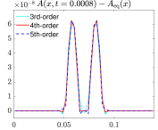
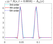
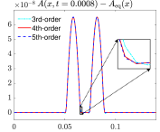
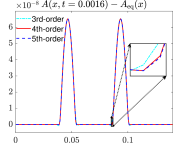
Figure 4.1: Example 3: Time snapshots of the difference $A(x,t)-A_{\rm eq}(x)$ computed on a coarse mesh (top row) and a fine mesh (bottom row).

Example 4—Non-zero-velocity “moving-blood” steady states

In the fourth example, we demonstrate how the proposed hybrid WB schemes preserve the non-zero steady state (3.1). We examine three distinct cases corresponding to the physiological conditions of an aneurysm, a stenosis, and a decreasing step. The initial conditions for each case are determined from the steady-state condition (3.1), which is expressed as

$$Q_{\rm s}=Q_{\rm in},\quad E_{\rm s}=\frac{(Q_{\rm in})^{2}}{2(A_{\rm out})^{2}}+\beta(\sqrt{A_{\rm out}}-\sqrt{A_{0}(L)}),$$ (4.4)

where the subscripts “in” and “out” denote values at the inlet (left side) and outlet (right side) of the domain, respectively, with $L$ representing the length of the artery (set to $0.16m$ in this example). In (4.4), the values of $A_{\rm in}$, $A_{\rm out}$, and $Q_{\rm in}$ are given by

$$A_{\rm in}=A_{0}(0)[1+S_{\rm in}]^{2},\quad A_{\rm out}=A_{0}(L)[1+S_{\rm in}]^{2},\quad Q_{\rm in}=A_{\rm in}S_{\rm in}C_{\rm in},$$

where $S_{\rm in}$ is the Shapiro number at the inlet, equivalent to the Froude number for the shallow water equations. For all test cases considered here, we set $S_{\rm in}=\{0.5,0.1,0.01\}$, given that blood flow is typically subcritical. Additionally, $C_{\rm in}$ denotes the Moens-Korteweg velocity at the inlet, defined as

$$C_{\rm in}=\sqrt{\frac{\kappa\sqrt{A_{\rm in}}}{2\rho\sqrt{\pi}}}.$$

Test 1: An aneurysm

In this test, we simulate an artery with an aneurysm by defining the cross-sectional radius at rest (see Figure 4.2, left) as

$$R_{0}(x)=\left\{\begin{aligned} &R_{\rm in},&&x\in[0,x_{1}]\cup[x_{4},L],\\ &R_{\rm in}+\frac{\Delta R}{2}\left[1-\cos\Big{(}\frac{x-x_{1}}{x_{2}-x_{1}}\pi\Big{)}\right],&&x\in[x_{1},x_{2}],\\ &R_{\rm in}+\Delta R,&&x\in[x_{2},x_{3}],\\ &R_{\rm in}+\frac{\Delta R}{2}\left[1+\cos\Big{(}\frac{x-x_{3}}{x_{4}-x_{3}}\pi\Big{)}\right],&&x\in[x_{3},x_{4}],\end{aligned}\right.$$

where $R_{\rm in}=4\times 10^{-3}m$, $\Delta R=1\times 10^{-3}m$, $x_{1}=\frac{9L}{40}$, $x_{2}=\frac{L}{4}$, $x_{3}=\frac{3L}{4}$, $x_{4}=\frac{31L}{40}$, and the cross-sectional area at rest is given by $A_{0}(x)=\pi(R_{0}(x))^{2}$. The initial profile of cross-sectional area $A(x,0)$ is determined by solving (4.4). With the obtained $A(x,0)$ and $Q(x,0)=Q_{\rm in}$, we run the simulation on a uniform mesh of $50$ cells until a final time $t=5$. The $L^{1}$- and $L^{\infty}$-errors are shown in Table 4.5, indicating that all errors are within machine accuracy, thus demonstrating the well-balanced property for “moving-blood” flow with an aneurysm is indeed maintained.

Table 4.5: Example 4—Test 1: $L^{1}$- and $L^{\infty}$-errors computed with parabolic, cubic, and quartic polynomials, for the equilibrium flow in an aneurysm.

$S_{\rm in}$	Var.	$r=2$		$r=3$		$r=4$
		$L^{1}$-error	$L^{\infty}$-error	$L^{1}$-error	$L^{\infty}$-error	$L^{1}$-error	$L^{\infty}$-error
$0.5$	$A$	9.54e-22	1.36e-20	2.07e-16	1.59e-15	2.65e-16	2.00e-15
	$Q$	3.47e-22	1.08e-19	4.88e-15	3.05e-14	5.67e-15	3.54e-14
$0.1$	$A$	1.17e-21	1.36e-20	3.45e-17	2.39e-16	7.72e-17	5.31e-16
	$Q$	1.47e-19	1.95e-18	2.34e-16	1.47e-15	2.38e-16	1.49e-15
$0.01$	$A$	7.28e-20	5.42e-19	2.03e-17	1.40e-16	7.09e-17	4.89e-16
	$Q$	2.48e-17	1.58e-16	1.33e-16	3.68e-17	3.00e-17	1.95e-16

Test 2: A Stenosis

In this test, we simulate an artery with a stenosis by defining the cross-sectional radius at rest (see Figure 4.2, middle) as

$$R_{0}(x)=\left\{\begin{aligned} &R_{\rm in},&&x\in[0,x_{1}]\cup[x_{2},L],\\ &R_{\rm in}-\frac{\Delta R}{4}\bigg{[}1-\cos\Big{(}2\pi\frac{x-x_{1}}{x_{2}-x_{1}}\Big{)}\bigg{]},&&x\in[x_{1},x_{2}],\end{aligned}\right.$$

where $x_{1}=\frac{3L}{10}$ and $x_{2}=\frac{7L}{10}$. We repeat the simulation as in Test 1, and show the $L^{1}$- and $L^{\infty}$-errors in Table 4.6, which validates the well-balanced property for “moving-blood” flow with a stenosis.

Table 4.6: Example 4—Test 2: Same as in Table 4.5 but for the flow in a stenosis.

$S_{\rm in}$	Var.	$r=2$		$r=3$		$r=4$
		$L^{1}$-error	$L^{\infty}$-error	$L^{1}$-error	$L^{\infty}$-error	$L^{1}$-error	$L^{\infty}$-error
$0.5$	$A$	2.04e-21	2.71e-20	1.30e-16	9.62e-16	1.81e-16	1.30e-15
	$Q$	2.08e-21	1.08e-19	4.97e-15	3.11e-14	5.88e-15	3.67e-14
$0.1$	$A$	2.60e-22	2.03e-20	2.54e-17	1.64e-16	6.24e-17	4.00e-16
	$Q$	4.64e-21	4.34e-19	1.92e-16	1.20e-15	2.23e-16	1.40e-15
$0.01$	$A$	6.85e-21	7.45e-20	1.08e-17	6.93e-17	5.40e-17	3.47e-16
	$Q$	4.06e-17	2.59e-16	1.38e-17	8.95e-17	1.72e-17	1.09e-16

Test 3: A decreasing step

In this test, we examine a scenario where the artery’s radius undergoes an instantaneous reduction, representing the transition from a parent to a daughter artery. This idealized transition results in a sudden change in the cross-sectional radius at a specific location. The radius at rest (see Figure 4.2, right) is defined as

$$R_{0}(x)=\left\{\begin{aligned} &R_{\rm in},&&x<\frac{L}{2},\\ &R_{\rm in}-\frac{\Delta R}{2},&&x\geq\frac{L}{2}.\end{aligned}\right.$$

Following the procedures of Tests 1 and 2, we compute the numerical solution up to a final time $t=5$ and present the $L^{1}$ and $L^{\infty}$ errors in Table 4.7. These results confirm the exact preservation of the “moving-blood” flow during the decreasing step.

Table 4.7: Example 4—Test 3: Same as in Tables 4.5 and 4.6 but for the flow in a decreasing step.

$S_{\rm in}$	Var.	$r=2$		$r=3$		$r=4$
		$L^{1}$-error	$L^{\infty}$-error	$L^{1}$-error	$L^{\infty}$-error	$L^{1}$-error	$L^{\infty}$-error
$0.5$	$A$	1.08e-21	1.36e-20	1.91e-16	1.45e-15	2.64e-16	1.95e-15
	$Q$	8.67e-21	1.08e-19	4.00e-15	2.52e-14	4.98e-15	3.12e-14
$0.1$	$A$	0	0	2.15e-17	1.46e-16	6.36e-17	4.23e-16
	$Q$	0	0	2.59e-16	1.62e-15	1.72e-16	1.08e-15
$0.01$	$A$	1.04e-21	1.36e-20	3.69e-17	2.45e-16	6.40e-17	4.26e-16
	$Q$	2.63e-19	3.96e-18	3.58e-16	2.24e-15	1.58e-16	9.90e-16

     

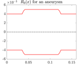
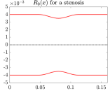
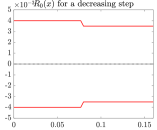
Figure 4.2: Example 4: Radii at rest for the artery with an aneurysm (left), a stenosis (middle), and a decreasing step (right).

Example 5—Small perturbation of “moving-blood” equilibrium in an aneurysm

In the fifth example, we demonstrate that the ability of the proposed arbitrarily high-order schemes in handling small perturbation to “moving-blood” steady state flow in an aneurysm. The background steady-state solution is given in Example 4, Test 1. We will denote the steady-state cross-sectional area as $A_{\rm eq}(x)$ and the steady-state discharge as $Q_{\rm eq}(x)$ here. We then introduce the perturbed initial conditions as follows:

$$A(x,0)=A_{\rm eq}(x)+\left\{\begin{aligned} &\varepsilon\pi\cos^{2}\Big{(}\frac{125\pi}{2}x\Big{)}&&\mbox{if}~{}x\in[0.072,0.088],\\ &0&&\mbox{otherwise},\end{aligned}\right.\quad Q(x,0)=Q_{\rm eq}(x),$$

defined within a computational domain $[0,0.16]$. Here, $\varepsilon=5\times 10^{-5}$ is a small magnitude number.

We compute the numerical solution by the third-, fourth-, and fifth-order schemes with either 50 or 200 uniform cells. The time snapshots of solution at $t=0.0025$ and $t=0.005$ are presented in Figures 4.3, 4.4, and 4.5, corresponding to $S_{\rm in}=0.5$, $0.1$, and $0.01$, respectively. As one can see, the proposed arbitrarily high-order schemes accurately capture the perturbations, consistent with results reported in [10]. Differences between the schemes are more pronounced with coarse mesh resolutions but diminish as the mesh is refined.

    

    

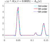
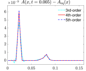
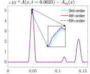
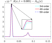
Figure 4.3: Example 5: Time snapshots of the difference $A(x,t)-A_{\rm eq}(x)$ for $S_{\rm in}=0.5$ and computed on a coarse mesh with 50 uniform cells (top row) and a fine mesh with 200 uniform cells (bottom row).

    

    

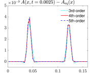
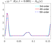
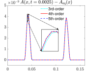
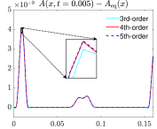
Figure 4.4: Example 5: Same as in Figure 4.3 but for $S_{\rm in}=0.1$.

    

    

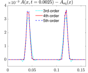
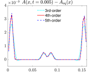
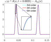
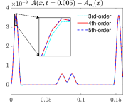
Figure 4.5: Example 5: Same as in Figures 4.3 and 4.4 but for $S_{\rm in}=0.01$.

Example 6—An ideal tourniquet problem

In the sixth example, we investigate the dynamics of an ideal tourniquet problem in blood flow. This is a scenario where a tourniquet is promptly applied and then subsequently removed. It is similar to the dam break problem in shallow water equations and the Sod tube problem in compressible gas dynamics. The computational domain spans $[-0.04,0.04]$, with the arterial stiffness number set to $\kappa=10^{7}\frac{Pa}{m}$, and the cross-sectional area at rest set as $A_{0}(x)=0$. The initial conditions are given by

$$A(x,0)=\left\{\begin{aligned} &\pi(5\times 10^{-3})^{2},&&x\in[-0.04,0],\\ &\pi(4\times 10^{-3})^{2},&&x\in[0,0.04],\end{aligned}\right.\quad Q(x,0)=0.$$

We compute the numerical solutions using the proposed third-, fourth-, and fifth-order schemes up to a final time $t=0.005$, employing a mesh size consisting of 50 uniform cells. Additionally, a reference solution is computed by the first-order Local Lax Fridriches’ scheme with 10000 uniform cells. Figure 4.6 presents the solutions, showcasing the well capture of the right-going shock wave and the left-going rarefaction. Moreover, the superiority of the high-order scheme becomes apparent upon closer inspection of the smooth rarefaction waves in the zoomed-in views.

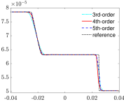
(a) A(x,t)

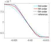
(b) zoom of A(x,t)

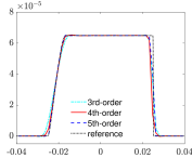
(c) Q(x,t)

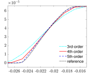
(d) zoom of Q(x,t)

Figure 4.6: Example 6: Numerical solutions of the cross-sectional area $A(x,t)$ (top row) and discharge $Q(x,t)$ (bottom row).

Example 7—Riemann problems

In the final example, we take the arterial stiffness number as $\kappa=5.87\times 10^{6}\frac{Pa}{m}$ and conduct numerical computations for two Riemann problems within the computational domain $[0,0.2]$. The cross-sectional area at rest is $A_{0}(x)=0$ and the initial conditions are given by

$$A(x,0)=6.28\times 10^{-4},\quad Q(x,0)=\left\{\begin{aligned} &-6.28\times 10^{-4},&&x\in[0,0.1],\\ &6.28\times 10^{-4},&&x\in[0.1,0.2],\end{aligned}\right.$$ (4.5)

and

$$A(x,0)=6.28\times 10^{-4},\quad Q(x,0)=\left\{\begin{aligned} &6.28\times 10^{-4},&&x\in[0,0.1],\\ &-6.28\times 10^{-4},&&x\in[0.1,0.2].\end{aligned}\right.$$ (4.6)

We perform numerical simulations using $100$ uniform cells for each of these two Riemann problems at final times $t=0.009$ and $t=0.012$, correspondingly. The computed results are presented in Figures 4.7 and 4.8, along with reference solutions obtained through the first-order Local Lax-Friedrichs’ scheme, employing a mesh comprising 10000 uniform cells. In Figure 4.7, the solution contains two rarefaction waves. Upon closer examination in the zoomed-in sections (right column of Figure 4.7), the superiority of high-order schemes is once again underscored. In Figure 4.8, the solution consists of two shock waves which are well captured without generating spurious oscillations by all three schemes.

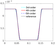
(a) A(x,t)

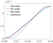
(b) zoom of A(x,t)

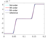
(c) Q(x,t)

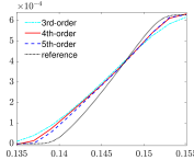
(d) zoom of Q(x,t)

Figure 4.7: Example 7: Numerical solutions of the cross-sectional area $A(x,t)$ (top row) and discharge $Q(x,t)$ (bottom row) for initial conditions (4.5).

(a) A(x,t)

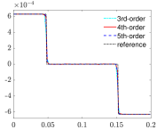
(b) Q(x,t)

Figure 4.8: Example 7: Numerical solutions of the cross-sectional area $A(x,t)$ (left) and discharge $Q(x,t)$ (right) for initial conditions (4.6).

Appendix A The RHS of (3.8)

In this appendix, we give the component-wise formulae of the RHS of (3.8). When a third-order scheme is considered, we have

$$\left\{\begin{aligned} &\big{(}F_{j}^{(0)}\big{)}^{[1]}+\big{(}S_{j}^{(0)}\big{)}^{[1]}=\frac{1}{\Delta x}\Big{[}Q_{e}^{j}(x_{j+\frac{1}{2}})-Q_{e}^{j}(x_{j-\frac{1}{2}})\Big{]},\\ &\big{(}F_{j}^{(0)}\big{)}^{[2]}+\big{(}S_{j}^{(0)}\big{)}^{[2]}=\frac{1}{\Delta x}\int_{K_{j}}\beta(A-A_{e}^{j})\big{(}\sqrt{A_{0}}\big{)}_{x}{\rm d}x\\ &\quad+\frac{1}{\Delta x}\left[\Big{(}\frac{(Q_{e}^{j}(x_{j+\frac{1}{2}}))^{2}}{A_{e}^{j}(x_{j+\frac{1}{2}})}+\frac{\beta}{3}\big{(}A_{e}^{j}(x_{j+\frac{1}{2}})\big{)}^{\frac{3}{2}}\Big{)}-\Big{(}\frac{(Q_{e}^{j}(x_{j-\frac{1}{2}}))^{2}}{A_{e}^{j}(x_{j-\frac{1}{2}})}+\frac{\beta}{3}\big{(}A_{e}^{j}(x_{j-\frac{1}{2}})\big{)}^{\frac{3}{2}}\Big{)}\right]\\ \end{aligned}\right.$$

When a fourth- and fifth-order schemes are taken into account, we additionally obtain

$$\left\{\begin{aligned} &\big{(}F_{j}^{(1)}\big{)}^{[1]}+\big{(}S_{j}^{(1)}\big{)}^{[1]}=\frac{4}{\Delta x^{2}}\int\limits_{K_{j}}\big{(}Q(x)-Q_{e}^{j}(x)\big{)}\,{\rm d}x+\frac{2}{\Delta x}\Big{[}Q_{e}^{j}(x_{j+\frac{1}{2}})+Q_{e}^{j}(x_{j-\frac{1}{2}})\Big{]},\\ &\big{(}F_{j}^{(1)}\big{)}^{[2]}+\big{(}S_{j}^{(1)}\big{)}^{[2]}=\frac{4}{\Delta x^{2}}\int\limits_{K_{j}}\left[\frac{Q^{2}}{A}+\frac{\beta}{3}A^{\frac{3}{2}}-\Big{(}\frac{(Q_{e}^{j})^{2}}{A_{e}^{j}}+\frac{\beta}{3}(A_{e}^{j})^{\frac{3}{2}}\Big{)}\right]\,{\rm d}x\\ &+\frac{2}{\Delta x}\left[\Big{(}\frac{(Q_{e}^{j}(x_{j+\frac{1}{2}}))^{2}}{A_{e}^{j}(x_{j+\frac{1}{2}})}+\frac{\beta}{3}\big{(}A_{e}^{j}(x_{j+\frac{1}{2}})\big{)}^{\frac{3}{2}}\Big{)}+\Big{(}\frac{(Q_{e}^{j}(x_{j-\frac{1}{2}}))^{2}}{A_{e}^{j}(x_{j-\frac{1}{2}})}+\frac{\beta}{3}\big{(}A_{e}^{j}(x_{j-\frac{1}{2}})\big{)}^{\frac{3}{2}}\Big{)}\right]\\ &+\frac{4}{\Delta x^{2}}\int_{K_{j}}\beta(A-A_{e}^{j})\big{(}\sqrt{A_{0}}\big{)}_{x}(x-x_{j}){\rm d}x,\end{aligned}\right.$$

and

$$\left\{\begin{aligned} &\big{(}F_{j}^{(2)}\big{)}^{[1]}+\big{(}S_{j}^{(2)}\big{)}^{[1]}=\frac{24}{\Delta x^{3}}\int\limits_{K_{j}}\big{(}Q(x)-Q_{e}^{j}(x)\big{)}(x-x_{j})\,{\rm d}x\\ &\quad+\frac{3}{\Delta x}\Big{[}Q_{e}^{j}(x_{j+\frac{1}{2}})-Q_{e}^{j}(x_{j-\frac{1}{2}})\Big{]},\\ &\big{(}F_{j}^{(2)}\big{)}^{[2]}+\big{(}S_{j}^{(2)}\big{)}^{[2]}=\frac{24}{\Delta x^{3}}\int\limits_{K_{j}}\left[\frac{Q^{2}}{A}+\frac{\beta}{3}A^{\frac{3}{2}}-\Big{(}\frac{(Q_{e}^{j})^{2}}{A_{e}^{j}}+\frac{\beta}{3}(A_{e}^{j})^{\frac{3}{2}}\Big{)}\right](x-x_{j})\,{\rm d}x\\ &+\frac{3}{\Delta x}\left[\Big{(}\frac{(Q_{e}^{j}(x_{j+\frac{1}{2}}))^{2}}{A_{e}^{j}(x_{j+\frac{1}{2}})}+\frac{\beta}{3}\big{(}A_{e}^{j}(x_{j+\frac{1}{2}})\big{)}^{\frac{3}{2}}\Big{)}-\Big{(}\frac{(Q_{e}^{j}(x_{j-\frac{1}{2}}))^{2}}{A_{e}^{j}(x_{j-\frac{1}{2}})}+\frac{\beta}{3}\big{(}A_{e}^{j}(x_{j-\frac{1}{2}})\big{)}^{\frac{3}{2}}\Big{)}\right]\\ &+\frac{12}{\Delta x^{3}}\int_{K_{j}}\beta(A-A_{e}^{j})\big{(}\sqrt{A_{0}}\big{)}_{x}(x-x_{j})^{2}{\rm d}x\end{aligned}\right.$$

References

- [1] R. Abgrall, A combination of Residual Distribution and the Active Flux formulations or a new class of schemes that can combine several writings of the same hyperbolic problem: application to the 1D Euler equation, Commun. Appl. Math. Comput., 5 (2023), pp. 370–402.
- [2] R. Abgrall and W. Barsukow, Extensions of Active Flux to arbitrary order of accuracy, ESAIM: Mathematical Modelling and Numerical Analysis, 57 (2023), pp. 991–1027.
- [3] , A hybrid finite element–finite volume method for conservation laws, Appl. Math. Comput., 447 (2023), p. 127846.
- [4] R. Abgrall and Y. Liu, A new approach for designing well-balanced schemes for the shallow water equations: a combination of conservative and primitive formulations. https://doi.org/10.48550/arXiv.2304.07809.
- [5] A. P. Avolio, Multi-branched model of the human arterial system, Med Biol Eng Comput, 18 (1980), pp. 709–718.
- [6] W. Barsukow, The active flux scheme for nonlinear problems, J. Sci. Comput., 86 (2021), p. 34. Paper No. 3.
- [7] W. Barsukow and J. P. Berberich, A well-balanced Active Flux method for the shallow water equations with wetting and drying, Commun. Appl. Math. Comput., (2023). https://doi.org/10.1007/s42967-022-00241-x.
- [8] P. J. Blanco, G. D. Ares, S. A. Urquiza, and R. A. Feijóo, On the effect of preload and pre-stretch on hemodynamic simulations: an integrative approach, Biomech Model Mechan, 15 (2016), pp. 593–627.
- [9] P. J. Blanco and R. A. Feijóo, A dimensionally-heterogeneous closed-loop model for the cardiovascular system and its applications, Med Eng Phys, 35 (2013), pp. 652–667.
- [10] J. Britton and Y. Xing, Well-balanced discontinuous Galerkin methods for the one-dimensional blood flow through arteries model with man-at-eternal-rest and living-man equilibria, Comput. Fluids, 203 (2020), p. 104493.
- [11] Y. Cao, A. Kurganov, Y. Liu, and R. Xin, Flux globalization based well-balanced path-conservative central-upwind schemes for shallow water models, J. Sci. Comput, 92 (2022). Paper No. 69, 31 pp.
- [12] M. J. Castro, A. Pardo Milanés, and C. Parés, Well-balanced numerical schemes based on a generalized hydrostatic reconstruction technique, Math. Models Methods Appl. Sci., 17 (2007), pp. 2055–2113.
- [13] M. J. Castro Díaz, J. A. López-García, and C. Parés, High order exactly well-balanced numerical methods for shallow water systems, J. Comput. Phys., 246 (2013), pp. 242–264.
- [14] L. Cea and M. E. Vázquez-cendón, Unstructured finite volume discretisation of bed frictionand convective flux in solute transport models linked to the shallow water equations, J.Comput. Phys., 231 (2012), pp. 3317–3339.
- [15] Y. Cheng, A. Chertock, M. Herty, A. Kurganov, and T. Wu, A new approach for designing moving-water equilibria preserving schemes for the shallow water equations, J. Sci. Comput., 80 (2019), pp. 538–554.
- [16] Y. Cheng and A. Kurganov, Moving-water equilibria preserving central-upwind schemes for the shallow water equations, Commun. Math. Sci., 14 (2016), pp. 1643–1663.
- [17] A. Chertock, S. Cui, A. Kurganov, and T. Wu, Well-balanced positivity preserving central-upwind scheme for the shallow water system with friction terms, Int. J. Numer. Methods Fluids, 78 (2015), pp. 355–383.
- [18] A. Chertock, A. Kurganov, X. Liu, Y. Liu, and T. Wu, Well-balancing via flux globalization: Applications to shallow water equations with wet/dry fronts, J. Sci. Comput., 90 (2022). Paper No. 9, 21 pp.
- [19] S. Chu and A. Kurganov, Flux globalization based well-balanced central-upwind scheme for one-dimensional blood flow models, Calcolo, 60 (2023), p. 2.
- [20] S. Clain, S. Diot, and R. Loubère, A high-order finite volume method for systems of conservation laws—multi-dimensional optimal order detection (MOOD), J. Comput. Phys., 230 (2011), pp. 4028–4050.
- [21] O. Delestre and P.-Y. Lagrée, A ’well-balanced’ finite volume scheme for blood flow simulation, Int. J. Numer. Methods Fluids, 72 (2013), pp. 177–205.
- [22] T. A. Eyman and P. L. Roe, Active flux, in 49th AIAA Aerospace Science Meeting, 2011.
- [23] , Active flux for systems, in 20th AIAA Computational Fluid Dynamics Conference, 2011.
- [24] L. Formaggia, J. Gerbeau, F. Nobile, and A. Quarteroni, On the coupling of 3D and 1D navier-Stokes equations for flow problems in compliant vessels, Comput. Methods Appl. Mech. Engrg., 191 (2001), pp. 561–582.
- [25] L. Formaggia, J. F. Gerbeau, F. Nobile, and A. Quarteroni, Numerical treatment of defective boundary conditions for the navier–Stokes equations, SIAM J. Numer. Anal., 40 (2002), pp. 376–401.
- [26] A. R. Ghigo, O. Delestre, J.-M. Fullana, and P.-Y. Lagré, Low-Shapiro hydrostatic reconstruction technique for bloodflow simulation in large arteries with varying geometrical andmechanical properties, J. Comput. Phys., 331 (2017), pp. 108–136.
- [27] B. Ghitti, C. Berthon, M. H. Le, and E. F. Toro, A fully well-balanced scheme for the 1D blood flow equations with friction source term, J. Comput. Phys., 421 (2020), p. 109750.
- [28] C. Helzel, D. Kerkmann, and L. Scandurra, A new ADER method inspired by the active flux method, J. Sci. Comput., 80 (2019), pp. 35–61.
- [29] C. Klingenberg, A. Kurganov, Y. Liu, and M. Zenk, Moving-water equilibria preserving HLL-type schemes forthe shallow water equations, Commun. Math. Res., 36 (2020), pp. 247–271.
- [30] A. Kurganov, Y. Liu, and R. Xin, Well-balanced path-conservative central-upwind schemes based on flux globalization, J. Comput. Phys., 474 (2023), p. 111773. 32 pp.
- [31] G. Li, O. Delestre, and L. Yuan, Well-balanced discontinuous Galerkin method and finite volume WENO scheme based on hydrostatic reconstruction for blood flow model in arteries., Int. J. Numer. Methods Fluids, 86 (2018), pp. 491–508.
- [32] X. Liu, X. Chen, S. Jin, A. Kurganov, and H. Yu, Moving-water equilibria preserving partial relaxation scheme for the Saint-Venant system, SIAM J. Sci. Comput., 42 (2020), pp. A2206–A2229.
- [33] V. Michel-Dansac, C. Berthon, S. Clain, and F. Foucher, A well-balanced scheme for the shallow-water equations with topography or Manning friction, J. Comput. Phys., 335 (2017), pp. 115–154.
- [34] L. O. Müller, C. Parés, and E. F. Toro, Well-balanced high-order numerical schemes for one-dimensional blood flow in vessels with varying mechanical properties, J. Comput. Phys., 242 (2013), pp. 53–85.
- [35] J. Murillo and P. García-Navarro, A Roe type energy balanced solver for 1d arterial blood flow and transport, Comput. Fluids, 117 (2015), pp. 149–167.
- [36] S. Noelle, Y. Xing, and C.-W. Shu, High-order well-balanced finite volume WENO schemes for shallow water equation with moving water, J. Comput. Phys., 226 (2007), pp. 29–58.
- [37] M. S. Olufsen, C. S. Peskin, W. Y. Kim, E. M. Pedersen, A. Nadim, and J. Larsen, Numerical simulation and experimental validation of blood flow in arteries with structured-tree outflow conditions, Ann Biomed Eng, 28 (2000), pp. 1281–1299.
- [38] M. F. O’Rourke and A. P. Avolio, Pulsatile flow and pressure in human systemic arteries: studies in man and in a multibranched model of the human systemic arterial tree, Circ. Res., 46 (1980), pp. 363–372.
- [39] K. H. Parker and C. J. H. Jones, Forward and backward running waves in the arteries: analysis using the method of characteristics, J. Biomech. Eng., 112 (1990), pp. 322–326.
- [40] E. Pimentel-García, L. O. Müller, E. F. Toro, and Parés, High-order fully well-balanced numerical methods for one-dimensional blood flow with discontinuous properties, J. Comput. Phys., 475 (2023), p. 111869.
- [41] G. Pontrelli, A mathematical model of flow in a liquid-filled visco-elastic tube, Med Biol Eng Comput, 40 (2002), pp. 550–556.
- [42] , Nonlinear pulse propagation in blood flow problems, (2002), pp. 630–635. In: Anile AM, Capasso V, Greco A, editors. Progress in Industrial Mathematics at ECMI 2000. Berlin, Heidelberg: Springer Berlin Heidelberg.
- [43] A. Quarteroni, A. Manzoni, and C. Vergara, The cardiovascular system: mathematical modelling, numerical algorithms and clinical applications, Acta Numerica, 26 (2017), pp. 365–590.
- [44] A. Quarteroni, M. Tuveri, and A. Veneziani, Computational vascular fluid dynamics: problems, models and methods, Comput. Vis. Sci., 2 (2000), pp. 163–197.
- [45] S. J. Sherwin, L. Formaggia, J. Peiró, and V. Franke, Computational modelling of 1d blood flow with variable mechanical properties and its application to the simulation of wave propagation in the human arterial system, Internat. J. Numer. Methods Fluids, 43 (2003), pp. 673–700.
- [46] S. J. Sherwin, V. Franke, J. Peiró, and K. Parker, One-dimensional modelling of a vascular network in space-time variables, J. Engrg. Math., 47 (2003), pp. 217–250.
- [47] Y. Shi, P. Lawford, and R. Hose, Review of Zero-D and 1-D models of blood flow in the cardiovascular system, Biomed. Eng. Online, 10 (2011), p. 33.
- [48] E. F. Toro, Brain venous haemodynamics, neurological diseases and mathematical modelling. a review, Appl. Math. Comput., 272 (2016), pp. 542–579.
- [49] F. Vilar, A posterior correction of high-order discontinuous Galerkin scheme through subcell finite volume formulation and flux reconstruction, J. Comput. Phys., 387 (2019), pp. 245–279.
- [50] Z. Wang, G. Li, and O. Delestre, Well-balanced finite difference weighted essentially non-oscillatory schemes for the blood flow model, Internat. J. Numer. Methods Fluids, 82 (2016), pp. 607–622.
- [51] Y. Xing, Exactly well-balanced discontinuous Galerkin methods for the shallow water equations with moving water equilibrium, J. Comput. Phys., 257 (2014), pp. 536–553.
- [52] Y. Xing and C.-W. Shu, A survey of high order schemes for the shallow water equations, J. Math. Study, 47 (2014), pp. 221–249.
- [53] Z. Xu and C.-W. Shu, A high-order well-balanced alternative finite difference WENO (A-WENO) method with the exact conservation property for systems of hyperbolic balance laws, (2024). https://bpb-us-w2.wpmucdn.com/sites.brown.edu/dist/0/348/files/2023/07/A-high-order-well-balanced-alternative-finite-difference-WENO-A-WENO-method-with-the-exact-conservation-property.pdf.
- [54] , A high-order well-balanced discontinuous Galerkin method for hyperbolic balance laws based on the Gauss-Lobatto quadrature rules, (2024). https://bpb-us-w2.wpmucdn.com/sites.brown.edu/dist/0/348/files/2023/09/A-high-rder-well-balanced-discontinuous-Galerkin-method-for-hyperbolic-balance-laws.pdf.