Azimuthal geodesics in closed FLRW cosmologies II
Abstract
We study azimuthal geodesics in closed Friedmann-Lemâitre-Robertson-Walker (FLRW) cosmological models and give the angular distance travelled by a test particle moving along such a geodesic during one cycle of expansion and re-collapse of the universe. We extend previous results regarding the path followed by light rays to the two-fluid case, also including a cosmological constant, as well as to massive test particles.
1 Introduction
The Friedmann-Lemaître-Robertson-Walker (FLRW) spacetimes are four-dimensional models satisfying the cosmological principle, which states that the universe is homogeneous and isotropic. They are solutions to the Einstein field equations of General Relativity (GR) with energy-momentum content given by perfect, barotropic fluids, with linear equation of state , for a constant . They provide a robust mathematical framework for modelling the large-scale structure of our expanding universe[1, 2, 3, 4, 5]. Named after its contributors [6, 7, 8, 9, 10, 11], the FLRW metric describes a maximally symmetric space of constant curvature evolving in size. The curvature of the spatial surfaces dictates the geometry of the universe on cosmic scales [12, 13, 14], and the size is governed by a scale factor which appears in the metric.
The spatial curvature can take one of three forms: negative, zero, or positive, corresponding to an open, flat, or closed universe, respectively. The geometry of a closed universe, which is spatially a sphere, allows for a scenario in which the universe expands up to a maximum size, before recollapsing during the so-called big crunch. This oscillatory behaviour was first noted by Friedmann [6]. In the realm of cosmology, the concept of oscillating universes has been a subject of theoretical exploration. Notably, in [15], Harrison provided a classification for FLRW models, including oscillatory universes. These models of a universe undergoing cycles of expansion and contraction were also further explored in [16, 17, 18, 19]. In particular, in [20], the closed-universe recollapse conjecture—which states that, under certain conditions, the expanding universe could eventually reverse its course, contracting back to a highly dense state, and initiating a new cycle of expansion and contraction—was proposed as a potential solution to cosmological issues, such as the singularity problem.
To obtain information regarding the scale factor, one can solve the Einstein field equations in the context of the FLRW metric. Some of the solutions to the cosmological field equations can be found in terms of elementary functions, see e.g. [21, 22]. However, in some cases (for example, involving terms such a cosmological constant, non-zero curvature, and a cosmological fluid) explicit solutions to the cosmological field equations have been obtained in terms of special functions, often encountered in problems within mathematical physics [23, 24, 25], such as elliptic functions [26, 27, 28, 29, 30, 31, 32].
While the prevailing observational evidence has strongly favoured a spatially flat universe over a closed one, recent observations have prompted a reconsideration of the possibility that the universe may in fact exhibit a closed geometry [33, 34, 35, 36, 37, 38, 39, 40, 41]. In this geometric setting, it is possible to study azimuthal geodesics, geodesics with constant azimuthal angle. In GR, azimuthal geodesics have been extensively studied in the context of rotating systems and settings involving spherical symmetry, for example the movement around massive objects such as black holes, e.g.[42], where special functions arise [43, 44]. Azimuthal geodesics within closed FLRW models were discussed in our recent work [45], which specifically focused on azimuthal null geodesics. We found that the angular distance travelled by a ray of light starting at the beginning of the universe during the expansion and recollapse is given by , for an arbitrary linear equation of state parameter . We now broaden the scope to encompass several other cases.
In particular, we begin our discussion, in Sec. 2, with azimuthal geodesics as well as the general formula for the angular distance travelled by a geodesic test particle in a closed FLRW spacetime. We first focus on the azimuthal distance travelled by a massless test particle in two-fluid cosmologies extending previous results, in Sec. 3. In Sec. 4, we consider the case in which one of the two fluids represents a cosmological constant. Einstein first introduced a positive cosmological constant in his field equations to achieve a static universe [46], and it is now a potential candidate for dark energy, responsible for the accelerated expansion of the universe, for a review see [47]. In Sec. 5, we turn to massive test particles in single fluid cosmologies. In most cases, these results have to be expressed in terms of special functions, in particular, elliptic and hypergeometric functions.
Notation.
In the following, we will set the speed of light and Newton’s constant to unity.
2 Azimuthal geodesics in closed FLRW spacetimes
In what follows, we are concerned with azimuthal geodesics in the closed () FLRW spacetime, described by the line element
| (2.1) |
A constant time slice of this spacetime corresponds to a 3-sphere, , a maximally symmetric three-dimensional space with constant positive curvature. The so-called scale factor evolves according to the Friedmann equations
| (2.2) | ||||
| (2.3) |
where the dot denotes the derivative with respect to cosmic time . The evolution of is determined by the energy-momentum content and we assume the universe to be filled with two perfect, barotropic fluids with equation of state , for , where is the energy density, is the pressure, and is the equation of state parameter. Equations (2.2) and (2.3) imply the energy-momentum conservation,
| (2.4) |
which is satisfied by each fluid component, and yields
| (2.5) |
where , for , is a constant of integration. We now define , and , for , and re-write Eq. (2.2) as
| (2.6) |
We can use Eq. (2.6) to derive the value of the angle travelled by a particle on an azimuthal geodesic during one cycle of expansion and re-collapse for a closed FLRW universe in terms of , for . The geodesic equations can be derived by considering the Lagrangian
| (2.7) |
with affine parameter . Note that for null geodesics and for timelike geodesics, respectively. For the metric (2.1), we have the Lagrangian
| (2.8) |
where the prime denotes the derivative with respect to .
We are interested in motion along the azimuthal -direction only, i.e. at constant values of and . For simplicity, we set and .
The Euler-Lagrange equation of the Lagrangian for the -coordinate, on the other hand, implies the existence of a constant of motion , which reads
| (2.9) |
and can be associated with the angular momentum of the particle moving along the geodesic. By combining together with Eq. (2.8), we find
| (2.10) |
By separating the variables, we then obtain the expression for the angle travelled by a particle moving along an azimuthal geodesic during the expansion and subsequent re-collapse of the universe. Assuming and symmetry with respect to the value of the cosmic time at which attains its maximum value , we find
| (2.11) |
By employing Eq. (2.6), this can be rewritten as
| (2.12) |
where the maximum value of the scale factor satisfies the conditions in Eq. (2.2) and in Eq. (2.3).
3 Massless particles in two-fluid cosmologies
As we can see from (2.5), the energy-momentum density evolves differently according to the equation of state parameter. In the case of a universe filled with two barotropic fluids, this means that one of the fluids may prevail for some time in the universe’s evolution. This approach allows for a more comprehensive understanding of the dynamics of the universe. For a review on multifluid cosmologies see e.g. [31]. Azimuthal geodesics for light-like particles in single-fluid cosmologies have been discussed previously [45]. Here, we return to the case of massless particles and now extend the approach to the two-fluid case.
For convenience, we use the rescaling
| (3.1) |
such that Eq. (2.6) can be re-written in terms of , and reads
| (3.2) |
Moreover, since is for null geodesics, Eq. (2.12) becomes
| (3.3) |
This integral can be given in terms of elementary functions only for specific choices of and . This is related to the Theorem of Chebyshev, see Appendix A.1.
3.1 Dust and radiation
For a universe filled with dust (, i.e. ) and radiation (, i.e. ), Eq. (3.3) yields
| (3.4) |
The maximum value of the scale factor can be found from Eq. (3.2) and is given by
| (3.5) |
Inserting this into Eq. (3.4) gives
| (3.6) |
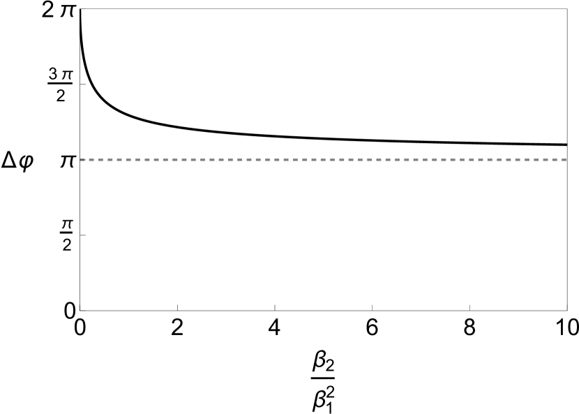
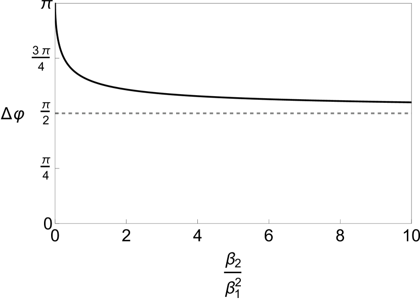
In Fig. 1(a) on p. 1, we show as a function of . The limit corresponds to a universe that contains only dust, for which we obtain , as expected. In the limit , which corresponds to a universe that contains only radiation, we find the known result .
3.2 Radiation and stiff matter
For a universe filled with radiation (, i.e. ) and stiff matter (, i.e. ), we find from Eq. (3.3)
| (3.7) |
The maximum value of the scale factor can be found from (3.2) and reads
| (3.8) |
Inserting this into Eq. (3.7) gives
| (3.9) |
In Fig. 1(b), we show in function of . The limit corresponds to a universe that contains only radiation, for which . In the limit , i.e. the limit corresponding to a universe filled only with stiff matter, we obtain .
Note that, mathematically, the case discussed here is similar to that for a dust and radiation filled universe, see Sec. 3.1. The reason is that the ratio in both cases.
3.3 Dust and stiff matter
Here, we consider a universe filled with dust (, i.e. ) and stiff matter (, i.e. ). Unlike the cases studied in Sec. 3.1 and Sec. 3.2, respectively, we now have and . The expression (3.3) then becomes
| (3.10) |
and is one of the roots of the polynomial
| (3.11) |
This is an integral which cannot be given in terms of elementary functions, but is elliptic.
The analytic expression for in this case is quite complicated since it involves a combination of the incomplete elliptic integrals of the first kind and of the third kind (see Appendix A.2 for more details), containing all the roots of . We remark that the discriminant of this polynomial is given by , since , this means that the polynomial has two real roots (one positive and one negative), and two complex conjugate roots. We denote these roots by , for , and is the largest positive real root, and find
| (3.12) |
where
| (3.13) |
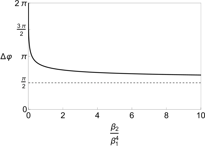
Noting that, for , the upper integration boundary gives the complete elliptic integrals of the first and third kind. We provide a plot of as a function of in Fig. 1(c). The behaviour of the function for small and large values of can be easily examined. As , we have
| (3.14) |
where we note that in this limit. We thus find that for ,
which is indeed consistent with the fact that as , we are in the limit .
For large values of , it is more helpful to return to the integral form containing and , and note that as , the integral becomes
4 Masless particle in a fluid with a cosmological constant
We will now discuss the azimuthal geodesics of a massless particle in a universe filled by matter, radiation, or stiff matter, together with a cosmological constant. To this end, we note that, for a cosmological constant , we can use (2.6) where we set and , or, equivalently, , effectively treating the cosmological constant as a fluid. In the following, we also set , , and, thus, . Note that for .
Before proceeding with our analysis, we seek the condition that the solution has to satisfy in order for it to be a positive real maximum. Equations (2.6) and (2.3) read
| (4.1) | ||||
| (4.2) |
Positive cosmological constant.
First we note that if is a (positive) maximum, then from Eq. (4.1), we can write
| (4.3) |
whence Eq. (4.2) reads
| (4.4) |
To ensure the existence of a (positive) maximum we require , which implies
| (4.5) |
In order to be able to make some more concrete statements, we need to fix the value of , and thus , and discuss the number of roots of Eq. (4.3).
Negative cosmological constant
We note that Eq. (4.2) does not yield a constraint for a maximum as for all , , and . However, this does not constitute a problem as it will be straightforward to identify the maximum in the specific scenarios.
4.1 Dust and cosmological constant
We now discuss the case of a universe filled with dust (, i.e. ) and a cosmological constant (, i.e. ). Equation (3.3) then reads
| (4.6) |
where . By letting , which implies , Eq. (4.6) becomes
| (4.7) |
where . We have thus obtained an elliptic integral in Weierstrass form (see Appendix A.3 for more details). Hence,
| (4.8) |
where is the inverse Weierstrass -function. The value of can be found from Eq. (3.2) by determining the roots of the third-degree polynomial in the scale factor , that is,
| (4.9) |
In the following, we will discuss the cases of the positive and the negative cosmological constant separately. The discriminant of the polynomial on the left-hand side of Eq. (4.9) is given by .
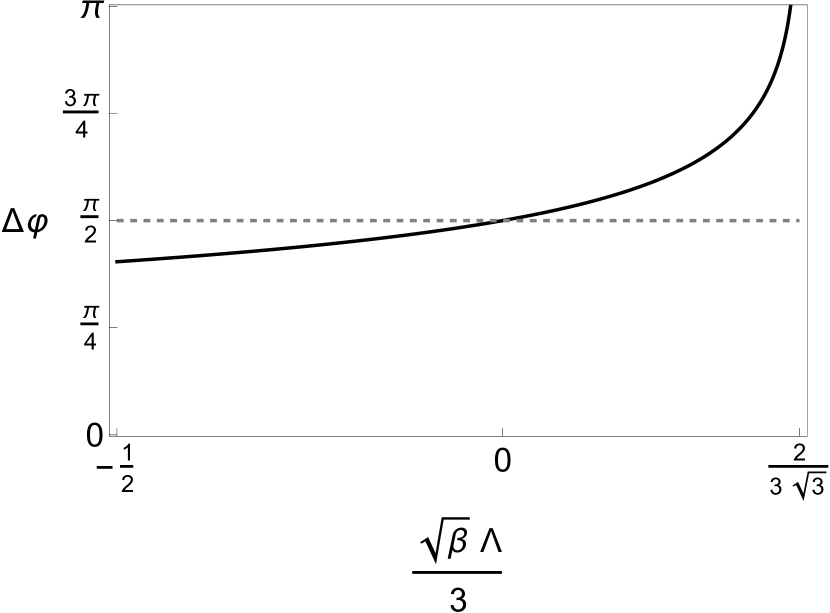
Positive cosmological constant ()
One can easily see that the depressed cubic polynomial in Eq. (4.9) has at least one negative real root and two complex conjugate roots if , i.e. ; and it has three real roots if , i.e. . We can therefore restrict our attention to the case , as other values would not lead to a closed universe. In the present case, from Eq. (4.5), we have an additional constraint on the value of
| (4.10) |
It can than be verified that the value of is given by
| (4.11) |
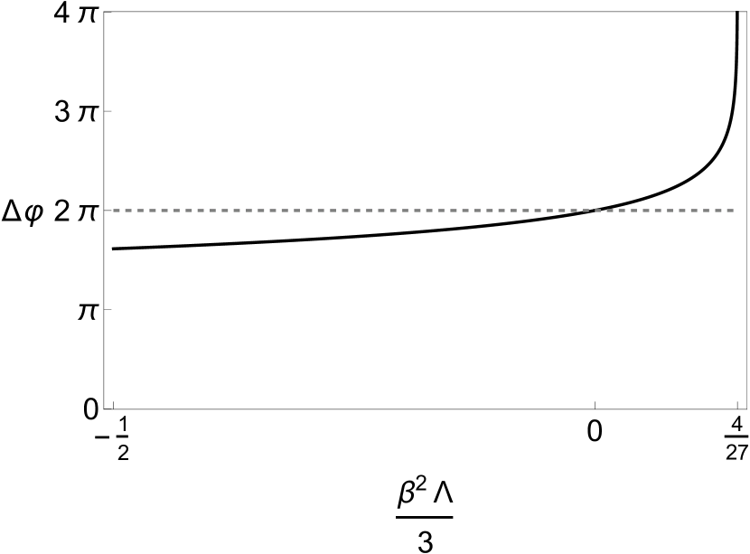
Note that although, at first glance, Eq. (4.11) appears to be complex (due to the square roots of negative terms), it is indeed real. In Fig. 2(a), we show the value of as a function of . We note that as , , while for , . This can also be verified by setting in the initial integral, Eq. (4.6). Physically, this means that, if the positive cosmological constant is dominant in the universe, closed universe solutions are no longer possible and, hence, the angular distance travelled by a massless particle on an azimuthal geodesic diverges.
Negative cosmological constant ()
We note that the discriminant, , is always negative in this case. This means that there is only one positive real root, which is our maximum, and two complex conjugate roots. In other words, for a negative cosmological constant, the universe always exhibits oscillatory behaviour. The value of is thus given by
| (4.12) |
We remark that, as , .
4.2 Radiation and cosmological constant
We now turn our attention to the case of a universe filled with radiation (, i.e. ) and a cosmological constant (, i.e. ). This gives
| (4.13) |
where , and is computed from
| (4.14) |
Equation (4.14) is bi-quadratic in , and the maximum real root is given by
| (4.15) |
for all values of . The value of then is
| (4.16) |
where is the complete elliptic integral of the first kind (see Appendix A.2).
Positive cosmological constant ()
It is clear that we require
| (4.17) |
Note that the root (4.15) satisfies the condition , from Eq. (4.5), and hence is, indeed, a maximum. The dependence of on is shown in Fig. 2(b). In the limit , we see that as expected. As , . The divergence again relates to the fact that, when the positive cosmological constant becomes too large, closed universe solutions no longer exist.
Negative cosmological constant ()
In this case, we have again no restriction on , and the universe always exhibits oscillatory behaviour. As , then decays to zero.
4.3 Stiff matter and cosmological constant
For stiff matter (, i.e. ) and a cosmological constant (, i.e. ), we get
| (4.18) |
where . The maximum value of corresponds to one of the roots of
| (4.19) |
and we denote it by , as usual. Let us perform the substitution
| (4.20) |
which allows us to re-write Eq. (4.18) as
| (4.21) | ||||
| (4.22) |
Note that if we take the limit in Eq. (4.18), we can easily find the value of which corresponds to that of a universe without a cosmological constant. Indeed, from Eq. (4.19) as , the maximum value of , and we have
Positive cosmological constant ()
We need to find a condition on which guarantees that the polynomial in Eq. (4.19) has a positive real root. This polynomial can be reduced to a cubic polynomial by letting , which is . A positive real root of Eq. (4.19) can arise only as the positive square root of a positive real root of . It is easy to check that it has exactly one negative real root, and so it has a positive real root if and only if it has more than one real root, i.e. if and only if it has non-negative discriminant. Its discriminant is , which is non-negative only if .
Therefore, when , the polynomial in Eq. (4.19) has two positive roots and two negative roots (these will be repeated roots when ). Further, we have the constraint from Eq. (4.5). It can be verified that the value of is given by
| (4.23) |
where . As in the case of Eq. 4.11, this is real-valued, despite appearing to be complex. Once again, this is a constraint on the positive cosmological constant. For larger values of , and hence of the cosmological constant, we do not have re-collapsing universes. In Fig. 2(c), we show as a function of .
Negative cosmological constant ()
Again, there is no restriction on and the only real positive root is given by
| (4.24) |
where is defined as above. As , then decays to zero.

5 Massive particles in single-fluid cosmologies
We shift our focus to the case of a massive particle in a closed FLRW universe, i.e. we choose in (2.11) and (2.12). We restrict our attention to single-fluid cosmologies, i.e. we set , , and , while . In this context, we do not study the case of a cosmological constant, since the physically relevant case of a positive cosmological constant does not lead to closed universe solutions. Recall that for dust, radiation, and stiff matter, respectively, the maximum value of the scale factor is given by
| (5.1) |
as shown in [45].
5.1 Dust
Here , i.e. , and consequently the integral to be evaluated reads
| (5.2) |
Recall that, in Sec. 2, we assumed to derive an expression for , and as it is an energy density. Note also that the integral is elliptic. We hence obtain
| (5.3) |
where is the complete elliptic integral of the first kind. In Fig. 3(a), we show as a function of the ratio between angular momentum and energy density . We find that as then . This is indeed consistent with the well-known result and the more general one we obtained in our recent work.
5.2 Radiation
In this case , i.e. , and hence
| (5.4) |
provided that . This integral is again elliptic. In Fig. 3(b) we show as a function of . For we find , as expected.
5.3 Stiff matter
For , i.e. , we have
| (5.5) | ||||
| (5.6) |
provided . Here is the generalised hypergeometric function (see A.4 for more details). In Fig. 3(c), we show as a function of . In the limit , this returns , which is consistent with our previous results.


6 Discussion and Conclusions
In this paper, we have extended our previous work [45] to find a closed formula for the azimuthal distance travelled by a massless or massive test particle, respectively, in a closed universe during one cycle of expansion and re-collapse. While an FLRW model does not allow closed universe solutions for a universe solely filled with a positive cosmological constant , two-fluid cosmologies allow us to include . This is, of course, possible as long as the positive cosmological constant does not dominate over the second fluid in such a way as to render closed universe solutions impossible. In our computations, we find that, as expected, diverges when we reach this limit. When considering a massless test particle moving in two-fluid cosmologies, we find that the integrals determining can be solved in terms of elementary functions only for a universe filled with (a) dust and radiation or (b) radiation and stiff matter (see Appendix A.1). All other cases lead to elliptic integrals. Extending these results to a massive test particle in a one-fluid model we find that for dust and radiation the value of is given in terms of the complete elliptic integral of the first kind with elliptic modulus depending on the energy density of the fluid and the angular momentum of the particle. For stiff matter, is a sum of such an elliptic integral and a generalised hypergeometric function with argument given in terms of the energy density of the stiff matter and the angular momentum of the test particle.
In principle, this work could be extended to other possible set-ups, e.g. to the motion of a massive test particle in two-fluid cosmologies. As suggested by the general expression for given here, this would likely involve hyperelliptic integrals or would require numerical tools.
Acknowledgments
Antonio d’Alfonso del Sordo is supported by the Engineering and Physical Sciences Research Council EP/R513143/1 & EP/T517793/1.
References
- [1] Supernova Search Team Collaboration, A. G. Riess et al., Observational evidence from supernovae for an accelerating universe and a cosmological constant, Astron. J. 116 (1998) 1009–1038, [astro-ph/9805201].
- [2] Supernova Cosmology Project Collaboration, S. Perlmutter et al., Measurements of and from 42 High Redshift Supernovae, Astrophys. J. 517 (1999) 565–586, [astro-ph/9812133].
- [3] E. L. Wright et al., Interpretation of the Cosmic Microwave Background radiation anisotropy detected by the COBE differential microwave radiometer, Astrophys. J. Lett. 396 (1992) L13–L18.
- [4] WMAP Collaboration, D. N. Spergel et al., Wilkinson Microwave Anisotropy Probe (WMAP) three year results: implications for cosmology, Astrophys. J. Suppl. 170 (2007) 377, [astro-ph/0603449].
- [5] Planck Collaboration, Y. Akrami et al., Planck 2018 results. VII. Isotropy and Statistics of the CMB, Astron. Astrophys. 641 (2020) A7, [arXiv:1906.02552].
- [6] A. Friedman, On the Curvature of space, Z. Phys. 10 (1922) 377–386.
- [7] G. Lemaitre, A Homogeneous Universe of Constant Mass and Growing Radius Accounting for the Radial Velocity of Extragalactic Nebulae, Annales Soc. Sci. Bruxelles A 47 (1927) 49–59.
- [8] H. P. Robertson, Kinematics and World-Structure, Astrophys. J. 82 (1935) 284–301.
- [9] H. P. Robertson, Kinematics and World-Structure. 2, Astrophys. J. 83 (1935) 187–201.
- [10] H. P. Robertson, Kinematics and World-Structure. 3, Astrophys. J. 83 (1936) 257–271.
- [11] A. G. Walker, On Milne’s Theory of World-Structure, Proc. Lond. Math. Soc. s 2–42 (1937), no. 1 90–127.
- [12] M. Lachieze-Rey and J.-P. Luminet, Cosmic topology, Phys. Rept. 254 (1995) 135–214, [gr-qc/9605010].
- [13] S. W. Hawking and G. F. R. Ellis, The Large Scale Structure of Space-Time. Cambridge Monographs on Mathematical Physics. Cambridge University Press, 2, 2023.
- [14] J. B. Griffiths and J. Podolsky, Exact Space-Times in Einstein’s General Relativity. Cambridge Monographs on Mathematical Physics. Cambridge University Press, Cambridge, 2009.
- [15] E. R. Harrison, Classification of Uniform Cosmological Models, Mon. Not. Roy. Astron. Soc. 137 (1967) 69–79.
- [16] J. D. Barrow and M. P. Dabrowski, Oscillating Universes, Mon. Not. Roy. Astron. Soc. 275 (1995) 850–862.
- [17] J. D. Barrow, D. Kimberly, and J. Magueijo, Bouncing universes with varying constants, Class. Quant. Grav. 21 (2004) 4289–4296, [astro-ph/0406369].
- [18] R. Brandenberger and P. Peter, Bouncing Cosmologies: Progress and Problems, Found. Phys. 47 (2017), no. 6 797–850, [arXiv:1603.05834].
- [19] J. D. Barrow and C. Ganguly, The Shape of Bouncing Universes, Int. J. Mod. Phys. D 26 (2017), no. 12 1743016, [arXiv:1705.06647].
- [20] J. D. Barrow, G. J. Galloway, and F. J. Tipler, The closed-universe recollapse conjecture., Mon. Not. Roy. Astron. Soc. 223 (Dec., 1986) 835–844.
- [21] C. G. Böhmer, Introduction to General Relativity and Cosmology. Essential Textbooks in Physics. World Scientific, 12, 2016.
- [22] D. Baumann, Cosmology. Cambridge University Press, 7, 2022.
- [23] G. E. Andrews, R. Askey, R. Roy, R. Roy, and R. Askey, Special functions, vol. 71. Cambridge University Press, 1999.
- [24] J. V. Armitage and W. F. Eberlein, Elliptic functions, vol. 67. Cambridge University Press, 2006.
- [25] R. Halburd, Special functions, in LTCC Advanced Mathematics Series: Volume 6 Analysis and Mathematical Physics, ch. 4, pp. 109–138. World Scientific, 2017.
- [26] D. Edwards, Exact expressions for the properties of the zero-pressureFriedmann models, Mon. Not. Roy. Astron. Soc. 159 (Jan., 1972) 51.
- [27] D. Edwards, Exact Solutions for Friedmann Models with Radiation, Astrophys. Space Sci. 24 (Oct., 1973) 563–575.
- [28] R. Coquereaux and A. Grossmann, Analytic Discussion of Spatially Closed Friedmann Universes With Cosmological Constant and Radiation Pressure, Annals Phys. 143 (1982) 296.
- [29] J. D’Ambroise, Applications of Elliptic and Theta Functions to Friedmann-Robertson-Lemaitre-Walker Cosmology with Cosmological Constant, in MSRI summer graduate workshop: A Window into Zeta and Modular Physics, 8, 2009. arXiv:0908.2481.
- [30] S. Chen, G. W. Gibbons, Y. Li, and Y. Yang, Friedmann’s Equations in All Dimensions and Chebyshev’s Theorem, JCAP 12 (2014) 035, [arXiv:1409.3352].
- [31] V. Faraoni, S. Jose, and S. Dussault, Multi-fluid cosmology in Einstein gravity: analytical solutions, Gen. Rel. Grav. 53 (2021), no. 12 109, [arXiv:2107.12488].
- [32] A. E. Pavlov, Friedmann Cosmology in Elliptic Functions, Grav. Cosmol. 27 (2021), no. 4 403–408.
- [33] E. Di Valentino, A. Melchiorri, and J. Silk, Planck evidence for a closed Universe and a possible crisis for cosmology, Nature Astron. 4 (2019), no. 2 196–203, [arXiv:1911.02087].
- [34] W. Handley, Curvature tension: evidence for a closed universe, Phys. Rev. D 103 (2021), no. 4 L041301, [arXiv:1908.09139].
- [35] S. Vagnozzi, E. Di Valentino, S. Gariazzo, A. Melchiorri, O. Mena, and J. Silk, The galaxy power spectrum take on spatial curvature and cosmic concordance, Phys. Dark Univ. 33 (2021) 100851, [arXiv:2010.02230].
- [36] S. Vagnozzi, A. Loeb, and M. Moresco, Eppur è piatto? The Cosmic Chronometers Take on Spatial Curvature and Cosmic Concordance, Astrophys. J. 908 (2021), no. 1 84, [arXiv:2011.11645].
- [37] E. Di Valentino, A. Melchiorri, and J. Silk, Investigating Cosmic Discordance, Astrophys. J. Lett. 908 (2021), no. 1 L9, [arXiv:2003.04935].
- [38] S. Dhawan, J. Alsing, and S. Vagnozzi, Non-parametric spatial curvature inference using late-Universe cosmological probes, Mon. Not. Roy. Astron. Soc. 506 (2021), no. 1 L1–L5, [arXiv:2104.02485].
- [39] S. Anselmi, M. F. Carney, J. T. Giblin, S. Kumar, J. B. Mertens, M. O’Dwyer, G. D. Starkman, and C. Tian, What is flat CDM, and may we choose it?, JCAP 02 (2023) 049, [arXiv:2207.06547].
- [40] A. Glanville, C. Howlett, and T. M. Davis, Full-shape galaxy power spectra and the curvature tension, Mon. Not. Roy. Astron. Soc. 517 (2022), no. 2 3087–3100, [arXiv:2205.05892].
- [41] A. Semenaite, A. G. Sánchez, A. Pezzotta, J. Hou, A. Eggemeier, M. Crocce, C. Zhao, J. R. Brownstein, G. Rossi, and D. P. Schneider, Beyond – CDM constraints from the full shape clustering measurements from BOSS and eBOSS, Mon. Not. Roy. Astron. Soc. 521 (2023), no. 4 5013–5025, [arXiv:2210.07304].
- [42] S. Chandrasekhar, The mathematical theory of black holes. Oxford University Press, 1985.
- [43] C. Lämmerzahl and E. Hackmann, Analytical Solutions for Geodesic Equation in Black Hole Spacetimes, Springer Proc. Phys. 170 (2016) 43–51, [arXiv:1506.01572].
- [44] A. Cieślik and P. Mach, Revisiting timelike and null geodesics in the Schwarzschild spacetime: general expressions in terms of Weierstrass elliptic functions, Class. Quant. Grav. 39 (2022), no. 22 225003, [arXiv:2203.12401].
- [45] C. G. Boehmer, A. d’Alfonso del Sordo, and B. Hartmann, Azimuthal geodesics in closed FLRW cosmologies, arXiv:2401.04597.
- [46] A. Einstein, Cosmological Considerations in the General Theory of Relativity, Sitzungsber. Preuss. Akad. Wiss. Berlin (Math. Phys. ) 1917 (1917) 142–152.
- [47] E. J. Copeland, M. Sami, and S. Tsujikawa, Dynamics of dark energy, Int. J. Mod. Phys. D 15 (2006) 1753–1936, [hep-th/0603057].
- [48] P. Tchebichef, Sur l’intégration des différentielles irrationnelles., Journal de Mathématiques Pures et Appliquées (1853) 87–111.
- [49] E. A. Marchisotto and G.-A. Zakeri, An invitation to integration in finite terms, The College Mathematics Journal 25 (1994), no. 4 295–308.
- [50] P. F. Byrd and M. D. Friedman, Handbook of Elliptic Integrals for Engineers and Scientists, vol. 67 of Grundlehren der mathematischen Wissenschaften. Springer, 1971.
Appendix A Special functions
Special functions arise as indefinite integrals which cannot be expressed in terms of elementary functions and are ubiquitous in mathematical physics.
A.1 Chebyshev’s Theorem
Theorem 1.
The integral
| (A.1) |
admits a representation in terms of elementary functions if and only if at least one of , , is an integer.
All the other cases require the use of special functions.
A.2 Elliptic integrals
The incomplete elliptic integral of the first kind is defined as
| (A.2) |
The incomplete elliptic integral of the third kind is defined as
| (A.3) |
where in both cases . Note that both integrals are said to be complete when , i.e. when .
The complete elliptic integral of the first kind, , is defined as , and the complete elliptic integral of the third kind is defined as .
A.3 Inverse Weierstrass elliptic function
A.4 Hypergeometric function
The generalised hypergeometric function is defined by the power series
where . Here is the (rising) Pochhammer symbol, which is given by