Approximations of Rockafellians, Lagrangians, and Dual Functions Julio Deride Johannes O. Royset Department of Mathematics Daniel J. Epstein Department of Industrial and Systems Engineering Universidad Técnica Federico Santa María University of Southern California julio.deride@usm.cl royset@usc.edu

Abstract.  Solutions of an optimization problem are sensitive to changes caused by approximations or parametric perturbations, especially in the nonconvex setting. This paper investigates the ability of substitute problems, constructed from Rockafellian functions, to provide robustness against such perturbations. Unlike classical stability analysis focused on local changes around (local) minimizers, we employ epi-convergence to examine whether the approximating problems suitably approach the actual one globally. We show that under natural assumptions the substitute problems can be well-behaved in the sense of epi-convergence even though the actual one is not. We further quantify the rates of convergence that often lead to Lipschitz-kind stability properties for the substitute problems.

Keywords: stability, approximation theory, epi-convergence, Rockafellian, Lagrangian, duality. Date:

1 Introduction

Given the problem of minimizing $\varphi:\mathbb{R}^{n}\to\overline{\mathbb{R}}=[-\infty,\infty]$, we are often compelled to consider one or more approximating problems. The approximations may stem from imprecise implementation of conceptual operations such as integration of nontrivial functions and maximization over uncountable sets or from smoothing methods and penalty functions. Approximations also arise in sensitivity analysis as model parameters are perturbed, for example in an effort to identify the problem’s robustness to adversarial interference and data manipulation. Optimization problems are prone to instability, with seemingly minor approximations causing disproportional changes in minimizers, minimum values, and even level-sets; see for example [37, 40]. Fortunately, every optimization problem can be associated with many substitute problems, potentially possessing more desirable properties. In this context, we focus on the nonconvex case and develop sufficient conditions under which Rockafellian relaxations, Lagrangian relaxations, and dual problems are stable in a specific sense.

Stability of optimization problems can be viewed from different angles; see, for example, the monographs [33, 1, 10, 36, 16, 27]. Metric regularity and calmness give rise to local stability [23, 30]. Tilt-stability [31, 22, 26, 21] and full-stability [29, 28] endow local minimizers with Lipschitz-type properties under perturbations; see [14] for recent efforts in these directions. Aligned with the pioneering work in [7, 8, 9], this paper takes an alternative, global perspective afforded by epi-convergence and its quantification in terms of the truncated Hausdorff distance. With $\varphi^{\nu}:\mathbb{R}^{n}\to\overline{\mathbb{R}}$, $\nu\in\mathbb{N}=\{1,2,\dots\}$ being a sequence of approximating functions, a concerning situation arises when $\varphi^{\nu}$ fails to epi-converge to the actual function $\varphi$ as $\nu\to\infty$. In the absence of this basic convergence property, one cannot expect minimizers, minimum values, and level-sets of the approximations to approach those of the actual function; see [36, Chapter 7]. Nevertheless, Rockafellian relaxations, Lagrangian relaxations, and dual problems can be brought in and they often achieve the desirable convergence at quantifiable rates.

All these substitute problems stem from Rockafellian functions, which form the centerpiece of our development. By definition, a function $f:\mathbb{R}^{m}\times\mathbb{R}^{n}\to\overline{\mathbb{R}}$ is a Rockafellian for $g:\mathbb{R}^{n}\to\overline{\mathbb{R}}$ when $f(0,x)=g(x)$ for all $x\in\mathbb{R}^{n}$ [43, Section 5.A]. As seen below, epi-convergence of Rockafellians is a key property in the analysis of the various substitute problems and their approximations. This perspective can be traced back to [15], but was much extended, especially to infinite-dimensional spaces, by [3, 2, 4, 11, 12] using epi/hypo-convergence [6]. However, these references deal with convex Rockafellians and the resulting convex-concave Lagrangians. In the present paper, we examine Rockafellians in the nonconvex setting and also quantify the rate of convergence.

Suppose that $\{f,f^{\nu}:\mathbb{R}^{m}\times\mathbb{R}^{n}\to\overline{\mathbb{R}},\nu\in\mathbb{N}\}$ are Rockafellians for $\{\varphi,\varphi^{\nu},\nu\in\mathbb{N}\}$, respectively. They define the following substitute problems as alternatives to the actual problem of minimizing $\varphi$ and the approximating problem of minimizing $\varphi^{\nu}$; the notation applies throughout the paper:

The Rockafellian relaxations (given $y,y^{\nu}\in\mathbb{R}^{m}$)

$$\mathop{\rm minimize}_{u\in\mathbb{R}^{m},x\in\mathbb{R}^{n}}f_{y}(u,x), \mbox{ where }f_{y}(u,x)=f(u,x)-\langle y,u\rangle$$

$$\mathop{\rm minimize}_{u\in\mathbb{R}^{m},x\in\mathbb{R}^{n}}f^{\nu}_{y^{\nu}}(u,x), \mbox{ where }f^{\nu}_{y}(u,x)=f^{\nu}(u,x)-\langle y,u\rangle.$$

The Lagrangian relaxations (given $y,y^{\nu}\in\mathbb{R}^{m}$)

$$\mathop{\rm minimize}_{x\in\mathbb{R}^{n}}\,l(x,y), \mbox{ where }l(x,y)=\mathop{\rm inf}\nolimits_{u}f(u,x)-\langle y,u\rangle$$

$$\mathop{\rm minimize}_{x\in\mathbb{R}^{n}}\,l^{\nu}(x,y^{\nu}), \mbox{ where }l^{\nu}(x,y)=\mathop{\rm inf}\nolimits_{u}f^{\nu}(u,x)-\langle y,u\rangle.$$

The dual problems

$$\mathop{\rm maximize}_{y\in\mathbb{R}^{m}}\,\psi(y), \mbox{ where }\psi(y)=\mathop{\rm inf}\nolimits_{u,x}f(u,x)-\langle y,u\rangle$$

$$\mathop{\rm maximize}_{y\in\mathbb{R}^{m}}\,\psi^{\nu}(y), \mbox{ where }\psi^{\nu}(y)=\mathop{\rm inf}\nolimits_{u,x}f^{\nu}(u,x)-\langle y,u\rangle.$$

Since a Rockafellian is simply a parametrization of the underlying function, there are countless possible versions of these substitute problems with concrete examples following below. The concept of developing dual problems through parametrization was pioneered in [33, Chapter 29], with further developments in [34, 35], but the idea of embedding a problem within a parametric family extends back to [32]. The name “Rockafellian” emerges in [43, Chapter 5] and [38], with “bifunction,” “bivariate function,” and “perturbation function” also being used in the literature. At least for common choices of Rockafellians, the importance of Lagrangian relaxations and dual problems in optimization is well documented (see, e.g., [43, Chapter 5], [36, Chapter 11]). They often provide effective, alternative paths to solving and/or bounding the actual and approximating problems.

We refer to $f_{y}$ and $f^{\nu}_{y^{\nu}}$ as tilted Rockafellians as they are simply constructed from $f$ and $f^{\nu}$ by subtracting a linear term. The bivariate functions $l,l^{\nu}$ defining Lagrangian relaxations are called Lagrangians, with classical forms from nonlinear programming arising for special choices of Rockafellians; see Example 2.1 below. We refer to $y,y^{\nu}$ in Rockafellian and Lagrangian relaxations as multiplier vectors. The optimization of dual functions $\psi,\psi^{\nu}$ can be viewed as a process of finding the best multiplier vectors as Rockafellian and Lagrangian relaxations always provide lower bounds on the minimum value of their respective actual and approximating problems.

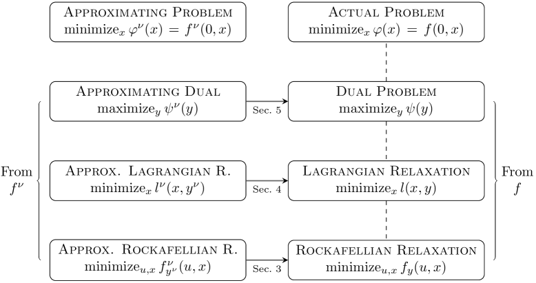
Figure 1: Actual and approximating problems and their substitutes defined by Rockafellians $f,f^{\nu}$.

Figure 1 provides a road map for the paper. The box in the upper-right corner represents an actual problem of minimizing $\varphi$. The absence of an arrow coming from the left indicates that the approximating functions $\varphi^{\nu}$ may fail to epi-converge to $\varphi$. A Rockafellian $f$ for $\varphi$ provides substitute problems listed on the right in Figure 1 that might be better behaved in the sense that if approximations are introduced in $f$ to produce $f^{\nu}$, a Rockafellian for $\psi^{\nu}$, then the resulting tilted Rockafellians $f_{y^{\nu}}^{\nu}$ epi-converge to $f_{y}$ and the Lagrangians $l^{\nu}(\cdot,y^{\nu})$ epi-converge to $l(\cdot,y)$ when $y^{\nu}\to y$. This is represented by the two lowest arrows in Figure 1. Likewise, we aspire to achieve hypo-convergence of the dual functions $\psi^{\nu}$ to $\psi$ as illustrated by a left-to-right arrow in the figure. (The shift from epi-convergence to hypo-convergence is dictated by the convention of stating dual problems in terms of maximization instead of minimization.) Without relying on convexity, we show that the convergences indicated by the horizontal arrows in the figure follow naturally when $f^{\nu}$ epi-converges to $f$ and that the rates can be quantified in a nonasymptotic analysis.

Even if the substitute problems on the left converge to those on the right in Figure 1 as just described, the fact remains that the substitute problems on the right are mere relaxations of the actual problem. However, we can rely on an extensive theory about strong duality (see, e.g., [36, Theorems 11.39, 11.59]), adjusted for our purpose in Definition 2.4 below, that posit conditions for “equivalence” among all four problems on the right-hand side in the figure as indicated by the dashed lines. Thus, we envision the analysis for an application to proceed in two steps: First, identify a Rockafellian $f$ such that equivalence is ensured on the right. Second, introduce the approximations to obtain $f^{\nu}$ and then confirm one or more of the “convergence arrows” from left to right. Even if the first step is not achieved, the substitute problems on the right-hand side are relaxations of the actual problem, and convergence to such relaxations by the approximations on the left-hand side can still be meaningful.

The paper summarizes the necessary background in Section 2. Section 3 addresses the convergence of tilted Rockafellians. Sections 4 and 5 discuss Lagrangians and dual functions, respectively.

Terminology. For any set $C$, $\iota_{C}(x)=0$ if $x\in C$ and $\iota_{C}(x)=\infty$ otherwise. We write $\operatorname{int}C$ for the interior of $C\subset\mathbb{R}^{n}$, $\operatorname{cl}C$ for the closure of $C$, and $\operatorname{bdry}C$ for the boundary of $C$, i.e., $\operatorname{bdry}C=\operatorname{cl}C\setminus\operatorname{int}C$. We write $X^{\nu}\,{\lower 1.0pt\hbox{$\rightarrow$}}\kern-10.0pt\hbox{\raise 4.0pt\hbox{$\,\scriptstyle s$}}\hskip 7.0ptX$ if the subsets $X^{\nu}\subset\mathbb{R}^{n}$ (Painlevé-Kuratowski) set-converges to $X\subset\mathbb{R}^{n}$.

For a function $g:\mathbb{R}^{n}\to\overline{\mathbb{R}}$, its domain $\operatorname{dom}g=\{x\in\mathbb{R}^{n}\,|\,g(x)<\infty\}$. Its epigraph is $\operatorname{epi}g=\{(x,\alpha)\in\mathbb{R}^{n}\times\mathbb{R}~{}|~{}f(x)\leq\alpha\}$. The minimum value of $g$ is $\inf g=\inf_{x}g(x)=\inf\{g(x)\,|\,x\in\mathbb{R}^{n}\}$ and the set of minimizers is written as $\mathop{\rm argmin}\nolimits g=\mathop{\rm argmin}\nolimits_{x}g(x)=\{x^{\star}\in\operatorname{dom}g\,|\,g(x^{\star})\leq\inf g\}$. For any $\varepsilon\in(0,\infty)$, the set of near-minimizers is written as $\varepsilon\mbox{-}\mathop{\rm argmin}\nolimits g=\{x^{\star}\in\operatorname{dom}g\,|\,g(x^{\star})\leq\inf g+\varepsilon\}$. We say that $g$ is proper when $g(x)>-\infty$ for all $x\in\mathbb{R}^{n}$ and $\operatorname{epi}g\neq\emptyset$. It is lower semicontinuous (lsc) when $\operatorname{epi}g$ is closed and it is convex if $\operatorname{epi}g$ is convex. We denote by $g^{*}$ the conjugate of $g$, i.e., $g^{*}(y)=\sup_{x}\langle x,y\rangle-g(x)$ for all $y\in\mathbb{R}^{n}$. The set of subgradients (in a general (limiting) sense) of $g$ at $x\in\mathbb{R}^{n}$ is denoted by $\partial g(x)$. A real-valued function $g:\mathbb{R}^{n}\to\mathbb{R}$ is Lipschitz continuous with modulus function $\kappa$ if $\kappa:[0,\infty)\to[0,\infty)$ and $|g(x)-g(\bar{x})|\leq\kappa(\rho)\|x-\bar{x}\|_{2}$ for all $x,\bar{x}\in\mathbb{B}(\rho)$ and $\rho\in[0,\infty)$.

For subsequence $N\subset\mathbb{N}$, we write $x^{\nu}\,{\raise 1.0pt\hbox{$\rightarrow$}}\kern-13.0pt\hbox{\lower 3.0pt\hbox{$\,\scriptstyle N$}}\hskip 7.0ptx$ when $\{x^{\nu},\nu\in N\}$ converges to $x$. We adopt the convention $\infty-\infty=\infty$; see also [43, Section 1.D]. Inequalities between vectors are interpreted componentwise.

2 Preliminaries

The dual function produced by a Rockafellian $f$ is $\psi=-f^{*}(\cdot,0)$ by definition, and the resulting Lagrangian $l$, for any $x$, has $-l(x,\cdot)$ as the conjugate of $f(\cdot,x)$. A concrete example from the far-reaching area of composite optimization (see, e.g., [19, 18, 39]) helps illustrate the concepts.

2.1 Example

(composite optimization). For $X,X^{\nu}\subset\mathbb{R}^{n}$, $g_{0},g_{0}^{\nu}:\mathbb{R}^{n}\to\mathbb{R}$, $G,G^{\nu}:\mathbb{R}^{n}\to\mathbb{R}^{m}$, and $h,h^{\nu}:\mathbb{R}^{m}\to\overline{\mathbb{R}}$, suppose that the actual and approximating problems are defined by

$$\varphi(x)=\iota_{X}(x)+g_{0}(x)+h\big{(}G(x)\big{)}~{}~{}~{}\mbox{ and }~{}~{}~{}\varphi^{\nu}(x)=\iota_{X^{\nu}}(x)+g_{0}^{\nu}(x)+h^{\nu}\big{(}G^{\nu}(x)\big{)}.$$

Even if each “component” $X$, $g_{0}$, $h$, and $G$ of the actual problem is approximated accurately by $X^{\nu}$, $g_{0}^{\nu}$, $h^{\nu}$, and $G^{\nu}$ respectively, $\varphi^{\nu}$ may not epi-converge to $\varphi$. For instance, this failure takes place in the simple nonlinear programming setting with $\varphi(x)=-x+\iota_{(-\infty,0]}(x^{3}-x^{2}-x+1)$ and $\varphi^{\nu}(x)=-x+\iota_{(-\infty,0]}(x^{3}-x^{2}-x+1+1/\nu)$; see [37, 39] for other problematic instances.

A possible Rockafellian for $\varphi$ and the resulting Lagrangian are given by

$$f(u,x)=\iota_{X}(x)+g_{0}(x)+h\big{(}G(x)+u\big{)}~{}~{}\mbox{ and }~{}~{}l(x,y)=\iota_{X}(x)+g_{0}(x)+\big{\langle}G(x),y\big{\rangle}-h^{*}(y),$$

with definitions of the approximating counterparts $f^{\nu}$ and $l^{\nu}$ following similarly. While $\varphi^{\nu}$ may not epi-converge to $\varphi$, we confirm that the resulting tilted Rockafellians $f_{y^{\nu}}^{\nu}$ epi-converge to $f_{y}$ (Proposition 3.2), the Lagrangians $l^{\nu}(\,\cdot\,,y^{\nu})$ epi-converge to $l(\,\cdot\,,y)$ (Subsection 4.2), and the dual functions $\psi^{\nu}$ hypo-converge to $\psi$ (Subsection 5.2) under natural assumptions. We also quantify the rate of convergence.

An explicit formula for the resulting dual function is available, for instance, when $X=\mathbb{R}^{n}$, $G(x)=Ax-b$, and $h(y)=\iota_{\{0\}^{m}}(y)$. Then, $\psi(y)=-\langle b,y\rangle-g_{0}^{*}(-A^{\top}y)$.

The main tool in the paper is epigraphical analysis; see [36, Chapter 7] for a comprehensive treatment. The functions $g^{\nu}:\mathbb{R}^{n}\to\overline{\mathbb{R}}$ epi-converge to $g:\mathbb{R}^{n}\to\overline{\mathbb{R}}$, written $g^{\nu}\,{\lower 1.0pt\hbox{$\rightarrow$}}\kern-10.0pt\hbox{\raise 4.0pt\hbox{$\,\scriptstyle e$}}\hskip 7.0ptg$, when

$$\forall x^{\nu}\to x,~{}~{}\mathop{\rm liminf}\nolimits g^{\nu}(x^{\nu})\geq g(x),$$ (2.1)

$$\forall x,~{}\exists x^{\nu}\to x\mbox{ with }\mathop{\rm limsup}\nolimits g^{\nu}(x^{\nu})\leq g(x).$$ (2.2)

We say that $\{g^{\nu},\nu\in\mathbb{N}\}$ is tight if for all $\varepsilon>0$, there exist compact $B_{\varepsilon}\subset\mathbb{R}^{n}$ and integer $\nu_{\varepsilon}\in\mathbb{N}$ such that $\mathop{\rm inf}\nolimits\{g^{\nu}(x)~{}|~{}x\in B_{\varepsilon}\}\leq\inf g^{\nu}+\varepsilon$ for all $\nu\geq\nu_{\varepsilon}$.

The consequences of epi-convergence are well known. The following facts can be proven using arguments nearly identical to those underpinning [43, Theorem 5.5].

2.2 Proposition

(consequences epi-convergence). For $\{g,g^{\nu}:\mathbb{R}^{n}\to\overline{\mathbb{R}},\nu\in\mathbb{N}\}$, the following hold:

1. If $\mathop{\rm liminf}\nolimits g^{\nu}(x^{\nu})\geq g(x)$ whenever $x^{\nu}\to x$ and $\{g^{\nu},\nu\in\mathbb{N}\}$ is tight, then $\mathop{\rm liminf}\nolimits(\inf g^{\nu})\geq\inf g$.

2. If for all $x\in\mathbb{R}^{n}$ there is $x^{\nu}\to x$ such that $\mathop{\rm limsup}\nolimits g^{\nu}(x^{\nu})\leq g(x)$, then $\mathop{\rm limsup}\nolimits(\inf g^{\nu})\leq\inf g$.

3. If $g^{\nu}\,{\lower 1.0pt\hbox{$\rightarrow$}}\kern-10.0pt\hbox{\raise 4.0pt\hbox{$\,\scriptstyle e$}}\hskip 7.0ptg$ and $\{g^{\nu},\nu\in\mathbb{N}\}$ is tight, then $\inf g^{\nu}\to\inf g$.

4. If $g^{\nu}\,{\lower 1.0pt\hbox{$\rightarrow$}}\kern-10.0pt\hbox{\raise 4.0pt\hbox{$\,\scriptstyle e$}}\hskip 7.0ptg$, $\inf g<\infty$, $x^{\nu}\in\varepsilon^{\nu}\mbox{-}\operatorname*{argmin}g^{\nu}$, $\varepsilon^{\nu}{\raise 1.0pt\hbox{$\scriptscriptstyle\,\searrow\,$}}0$, and $x^{\nu}\,{\raise 1.0pt\hbox{$\rightarrow$}}\kern-13.0pt\hbox{\lower 3.0pt\hbox{$\,\scriptstyle N$}}\hskip 7.0ptx$ for some subsequence $N\subset\mathbb{N}$, then $x\in\mathop{\rm argmin}\nolimits g$ and $g^{\nu}(x^{\nu})\,{\raise 1.0pt\hbox{$\rightarrow$}}\kern-13.0pt\hbox{\lower 3.0pt\hbox{$\,\scriptstyle N$}}\hskip 7.0pt\inf g$.

The functions $g^{\nu}:\mathbb{R}^{n}\to\overline{\mathbb{R}}$ hypo-converge to $g:\mathbb{R}^{n}\to\overline{\mathbb{R}}$, written $g^{\nu}\,{\lower 1.0pt\hbox{$\rightarrow$}}\kern-11.0pt\hbox{\raise 4.0pt\hbox{$\,\scriptstyle h$}}\hskip 7.0ptg$, when $-g^{\nu}\,{\lower 1.0pt\hbox{$\rightarrow$}}\kern-10.0pt\hbox{\raise 4.0pt\hbox{$\,\scriptstyle e$}}\hskip 7.0pt-g$, which then has immediate consequences for maximization problems.

A nonasymptotic analysis relies on the distance between two sets $C,D\subset\mathbb{R}^{n}$. For any norm $\|\cdot\|$ on $\mathbb{R}^{n}$, the excess of $C$ over $D$, if both sets are nonempty, is defined as $\operatorname{exs}(C;D)=\mathop{\rm sup}\nolimits_{x\in C}\inf_{y\in D}\|x-y\|$, while $\operatorname{exs}(C;\emptyset)=\infty$ for $C\neq\emptyset$ and $\operatorname{exs}(\emptyset;D)=0$ regardless of $D$. The centered ball $\mathbb{B}(\rho)=\{x\in\mathbb{R}^{n}~{}|~{}\|x\|\leq\rho\}$. For any $\rho\geq 0$, the truncated Hausdorff distance between $C$ and $D$ is

$$d\hat{\kern-1.49994ptl}_{\rho}(C,D)=\max\Big{\{}\operatorname{exs}\big{(}C\cap\mathbb{B}(\rho);~{}D\big{)},~{}~{}\operatorname{exs}\big{(}D\cap\mathbb{B}(\rho);~{}C\big{)}\Big{\}},$$

which depends on the norm underpinning the excess and the ball. The truncated Hausdorff distance quantifies epi-convergence [36, Theorem 7.57] but also results in the following fact, which essentially is [43, Theorem 6.56] under a trivial change of norm on $\mathbb{R}^{n}$. Thus, we omit a proof.

2.3 Proposition

(minimization error). For $g,h:\mathbb{R}^{n}\to\overline{\mathbb{R}}$, $\rho\in[0,\infty)$ and $\varepsilon\in[0,2\rho]$, suppose that

$$\mathop{\rm inf}\nolimits g,\mathop{\rm inf}\nolimits h\in[-\rho,\rho-\varepsilon],~{}~{}~{}~{}\mathop{\rm argmin}\nolimits g\cap\mathbb{B}(\rho)\neq\emptyset,~{}~{}~{}~{}\mathop{\rm argmin}\nolimits h\cap\mathbb{B}(\rho)\neq\emptyset,$$

using any norm $\|\cdot\|$ on $\mathbb{R}^{n}$. Adopt the norm $(x,\alpha)\mapsto(\max\{\|x\|,|\alpha|\}$ for $\mathbb{R}^{n+1}$. Then, one has

$$|\mathop{\rm inf}\nolimits g-\mathop{\rm inf}\nolimits h|\leq d\hat{\kern-1.49994ptl}_{\rho}(\operatorname{epi}g,\operatorname{epi}h)~{}~{}~{}\mbox{ and }~{}~{}~{}\operatorname{exs}\big{(}\varepsilon\mbox{-}\mathop{\rm argmin}\nolimits h\cap\mathbb{B}(\rho);~{}\delta\mbox{-}\mathop{\rm argmin}\nolimits g\big{)}\leq d\hat{\kern-1.49994ptl}_{\rho}(\operatorname{epi}g,\operatorname{epi}h)$$

provided that $\delta>\varepsilon+2d\hat{\kern-1.49994ptl}_{\rho}(\operatorname{epi}g,\operatorname{epi}h)$.

The usefulness of a dual problem depends in part on whether $\sup\psi=\inf\varphi$, a property which we refer to as strong duality. In Example 2.1, if $X$ is compact, $g_{0}$ is convex and lsc, $h$ is proper, lsc, and convex, and $\langle G(\cdot),y\rangle$ is convex for all $y\in\operatorname{dom}h^{*}$, then Sion’s theorem [44, Corollary 3.3] ensures strong duality; see [36, Theorems 11.39 and 11.59] for more general conditions.

We follow [40], which relies on exactness to confirm the equivalence between the problems on the right-hand side of Figure 1. The terminology is motivated by exact penalization [17], augmented Lagrangians [36, Section 11.K], and recent work on linear penalties [20]. While [36, Definition 11.60] identifies exactness as a Lagrangian $l(\cdot,y)$ having identical minimizers and minimum value to those of $\varphi$, we shift the focus to the min-value function $\inf_{x}f(\cdot,x)$ given by the underlying Rockafellian.

2.4 Definition

(exact Rockafellians). A Rockafellian $f:\mathbb{R}^{m}\times\mathbb{R}^{n}\to\overline{\mathbb{R}}$ for $\varphi:\mathbb{R}^{n}\to\overline{\mathbb{R}}$ is exact, supported by $y\in\mathbb{R}^{m}$, if

$$\mathop{\rm inf}\nolimits_{x}f(u,x)\geq\inf\varphi+\langle y,u\rangle~{}~{}~{}\forall u\in\mathbb{R}^{m}.$$ (2.3)

If the inequality holds strictly for all $u\neq 0$, then $f$ is strictly exact, supported by $y$.

In terms of the corresponding dual function $\psi$, the condition (2.3) holds if and only if $\psi(y)=\inf\varphi$ because generally $\psi(y^{\prime})\leq\inf\varphi$ for all $y^{\prime}\in\mathbb{R}^{m}$ and (2.3) amounts to having $\psi(y)=\inf f_{y}\geq\inf\varphi$. Consequently, when $f$ is exact for $\varphi$, supported by $y$, one has

$$\inf f_{y}=\mathop{\rm inf}\nolimits_{x}l(x,y)=\psi(y)=\sup\psi=\inf\varphi.$$ (2.4)

Thus, the problems on the right-hand side of Figure 1 are equivalent in the sense of optimal objective function values; see [40, Proposition 3.3] for further characterizations. Any Rockafellian $f$ can be augmented to produce a strictly exact Rockafellian $(u,x)\mapsto f(u,x)+\iota_{\{0\}^{m}}(u)$. Many other possibilities exist as well, including augmentation defined by norms; see [36, Section 11.K].

3 Convergence of Tilted Rockafellians

The convergence of Rockafellians and the rate carry over to those of their tilted counterparts, which formalizes the bottom arrow in Figure 1. We consider both general and specific settings.

3.1 General Results

The following theorem is noticeable by its lack of assumptions on the underlying Rockafellians and broadly justifies the consideration of approximating Rockafellian relaxations.

3.1 Theorem

(convergence of tilted Rockafellians). For Rockafellians $\{f,f^{\nu}:\mathbb{R}^{m}\times\mathbb{R}^{n}\to\overline{\mathbb{R}},\nu\in\mathbb{N}\}$, the following hold.

1. If $f^{\nu}\,{\lower 1.0pt\hbox{$\rightarrow$}}\kern-10.0pt\hbox{\raise 4.0pt\hbox{$\,\scriptstyle e$}}\hskip 7.0ptf$ and $y^{\nu}\to y\in\mathbb{R}^{m}$, then $f^{\nu}_{y^{\nu}}\,{\lower 1.0pt\hbox{$\rightarrow$}}\kern-10.0pt\hbox{\raise 4.0pt\hbox{$\,\scriptstyle e$}}\hskip 7.0ptf_{y}$.

2. If $\operatorname{epi}f$ and $\operatorname{epi}f^{\nu}$ are nonempty, $\rho\in[0,\infty)$, $y,y^{\nu}\in\mathbb{R}^{m}$, and $\bar{\rho}\geq\rho(1+\max\{\|y\|_{2},\|y^{\nu}\|_{2}\})$, then

   $$d\hat{\kern-1.49994ptl}_{\rho}(\operatorname{epi}f_{y},\operatorname{epi}f^{\nu}_{y^{\nu}})\leq\Big{(}1+\max\big{\{}\|y\|_{2},\|y^{\nu}\|_{2}\big{\}}\Big{)}d\hat{\kern-1.49994ptl}_{\bar{\rho}}(\operatorname{epi}f,\operatorname{epi}f^{\nu})+\rho\|y-y^{\nu}\|_{2},$$

   where the norm on $\mathbb{R}^{m}\times\mathbb{R}^{n}\times\mathbb{R}$ is $(u,x,\alpha)\mapsto\max\{\|u\|_{2},\|x\|_{2},|\alpha|\}$.

Proof. For (a), since $(u,x)\mapsto\langle y^{\nu},\cdot\,\rangle$ both epi-converges and hypo-converges to $(u,x)\mapsto\langle y,\cdot\,\rangle$ and the latter function is real-valued, we can follow the proof of [43, Proposition 4.19].

For (b), let $\varepsilon\in(0,\infty)$ and $(u^{\nu},x^{\nu},\alpha^{\nu})\in\operatorname{epi}f^{\nu}_{y^{\nu}}\cap\mathbb{B}(\rho)$. Thus, $f^{\nu}(u^{\nu},x^{\nu})\leq\alpha^{\nu}+\langle y^{\nu},u^{\nu}\rangle$ and

$$\big{|}\alpha^{\nu}+\langle y^{\nu},u^{\nu}\rangle\big{|}\leq|\alpha^{\nu}|+\|y^{\nu}\|_{2}\|u^{\nu}\|_{2}\leq\rho\big{(}1+\|y^{\nu}\|_{2}\big{)}\leq\bar{\rho}.$$

Since $(u^{\nu},x^{\nu},\alpha^{\nu}+\langle y^{\nu},u^{\nu}\rangle)\in\operatorname{epi}f^{\nu}\cap\mathbb{B}(\bar{\rho})$, there exist $(u,x,\alpha)\in\operatorname{epi}f$ such that

$$\max\big{\{}\|u-u^{\nu}\|_{2},\|x-x^{\nu}\|_{2},\big{\|}\alpha-\alpha^{\nu}-\langle y^{\nu},u^{\nu}\rangle\big{\|}_{2}\big{\}}\leq d\hat{\kern-1.49994ptl}_{\bar{\rho}}(\operatorname{epi}f,\operatorname{epi}f^{\nu})+\varepsilon.$$

With $\delta=d\hat{\kern-1.49994ptl}_{\bar{\rho}}(\operatorname{epi}f,\operatorname{epi}f^{\nu})+\varepsilon+\rho\|y-y^{\nu}\|_{2}+\|y\|_{2}(d\hat{\kern-1.49994ptl}_{\bar{\rho}}(\operatorname{epi}f,\operatorname{epi}f^{\nu})+\varepsilon)$, the point $(u,x)$ satisfies

$$f_{y}(u,x)\leq\alpha-\langle y,u\rangle\leq\alpha^{\nu}+\langle y^{\nu},u^{\nu}\rangle+d\hat{\kern-1.49994ptl}_{\bar{\rho}}(\operatorname{epi}f,\operatorname{epi}f^{\nu})+\varepsilon-\langle y,u\rangle\leq\alpha^{\nu}+\delta.$$

Since $\delta\in\mathbb{R}$, this means that $(u,x,\alpha^{\nu}+\delta)\in\operatorname{epi}f_{y}$ and its distance to $(u^{\nu},x^{\nu},\alpha^{\nu})$ (in the adopted norm) is at most $\delta$. Since $(u^{\nu},x^{\nu},\alpha^{\nu})\in\operatorname{epi}f^{\nu}_{y^{\nu}}\cap\mathbb{B}(\rho)$ is arbitrary, we find that $\operatorname{exs}(\operatorname{epi}f^{\nu}_{y^{\nu}}\cap\mathbb{B}(\rho);\operatorname{epi}f_{y})\leq\delta$. Since $\varepsilon$ is arbitrary, it also follows that

$$\operatorname{exs}\big{(}\operatorname{epi}f^{\nu}_{y^{\nu}}\cap\mathbb{B}(\rho);\operatorname{epi}f_{y}\big{)}\leq\Big{(}1+\max\big{\{}\|y\|_{2},\|y^{\nu}\|_{2}\big{\}}\Big{)}d\hat{\kern-1.49994ptl}_{\bar{\rho}}(\operatorname{epi}f,\operatorname{epi}f^{\nu})+\rho\|y-y^{\nu}\|_{2}.$$

After repeating the arguments with the roles of $f_{y}$ and $f^{\nu}_{y^{\nu}}$ reversed, we reach the conclusion.      

If $f$ is a Rockafellian for $\varphi:\mathbb{R}^{n}\to\overline{\mathbb{R}}$, then Theorem 3.1(a) and Proposition 2.2(b) allow us to conclude that $\mathop{\rm limsup}\nolimits(\inf f_{y^{\nu}}^{\nu})\leq\inf f_{y}\leq\inf\varphi$. Thus, the approximating Rockafellian relaxation is indeed a relaxation of the actual problem in the limit regardless of $y$ as long as $y^{\nu}\to y$. The rate of convergence of near-minimizers of approximating Rockafellian relaxations to those of a Rockafellian relaxation follows from Theorem 3.1(b) and Proposition 2.3.

3.2 Examples from Composite Optimization

We return to Example 2.1 and establish that $f^{\nu}\,{\lower 1.0pt\hbox{$\rightarrow$}}\kern-10.0pt\hbox{\raise 4.0pt\hbox{$\,\scriptstyle e$}}\hskip 7.0ptf$ at a quantifiable rate under natural assumptions.

3.2 Proposition

(composite optimization; epi-convergence). In the setting of Example 2.1, suppose that $X^{\nu}\,{\lower 1.0pt\hbox{$\rightarrow$}}\kern-10.0pt\hbox{\raise 4.0pt\hbox{$\,\scriptstyle s$}}\hskip 7.0ptX$, $h^{\nu}\,{\lower 1.0pt\hbox{$\rightarrow$}}\kern-10.0pt\hbox{\raise 4.0pt\hbox{$\,\scriptstyle e$}}\hskip 7.0pth$, with $h$ proper, and $g_{0}^{\nu}(x^{\nu})\to g_{0}(x)$ and $G^{\nu}(x^{\nu})\to G(x)$ whenever $x^{\nu}\in X^{\nu}\to x\in X$. Then, $f^{\nu}\,{\lower 1.0pt\hbox{$\rightarrow$}}\kern-10.0pt\hbox{\raise 4.0pt\hbox{$\,\scriptstyle e$}}\hskip 7.0ptf$.

Proof. We first consider the liminf-condition (2.1). Let $u^{\nu}\to u$ and $x^{\nu}\to x$. Since $X^{\nu}\,{\lower 1.0pt\hbox{$\rightarrow$}}\kern-10.0pt\hbox{\raise 4.0pt\hbox{$\,\scriptstyle s$}}\hskip 7.0ptX$, $\mathop{\rm liminf}\nolimits\iota_{X^{\nu}}(x^{\nu})\geq\iota_{X}(x)$. If $x\not\in X$, then this implies that $\mathop{\rm liminf}\nolimits\varphi^{\nu}(x^{\nu})\geq\varphi(x)$ because $h$ is proper. If $x\in X$, then we proceed without loss generality under the assumption that $x^{\nu}\in X^{\nu}$ because $f^{\nu}(u^{\nu},x^{\nu})=\infty$ otherwise. Thus, $g_{0}^{\nu}(x^{\nu})\to g_{0}(x)$ and $G^{\nu}(x^{\nu})\to G(x)$. Since $h^{\nu}\,{\lower 1.0pt\hbox{$\rightarrow$}}\kern-10.0pt\hbox{\raise 4.0pt\hbox{$\,\scriptstyle e$}}\hskip 7.0pth$, one has $\mathop{\rm liminf}\nolimits h^{\nu}(G^{\nu}(x^{\nu})+u^{\nu})\geq h(G(x)+u)$. We conclude that $\mathop{\rm liminf}\nolimits\varphi^{\nu}(x^{\nu})\geq\varphi(x)$ holds in this case too. Second, we consider the limsup-condition (2.2). Let $(u,x)\in\mathbb{R}^{m}\times\mathbb{R}^{n}$. Without loss of generality, we assume that $x\in X$. Since $X^{\nu}\,{\lower 1.0pt\hbox{$\rightarrow$}}\kern-10.0pt\hbox{\raise 4.0pt\hbox{$\,\scriptstyle s$}}\hskip 7.0ptX$, there is $x^{\nu}\in X^{\nu}\to x$. Also, since $h^{\nu}\,{\lower 1.0pt\hbox{$\rightarrow$}}\kern-10.0pt\hbox{\raise 4.0pt\hbox{$\,\scriptstyle e$}}\hskip 7.0pth$, there is $z^{\nu}$ $\to$ $G(x)+u$ such that $\mathop{\rm limsup}\nolimits h^{\nu}(z^{\nu})\leq h(G(x)+u)$. Set $u^{\nu}=z^{\nu}-G^{\nu}(x^{\nu})$. Then, $u^{\nu}\to u$. Moreover,

$$\mathop{\rm limsup}\nolimits f^{\nu}(u^{\nu},x^{\nu})\leq\mathop{\rm limsup}\nolimits g_{0}^{\nu}(x^{\nu})+\mathop{\rm limsup}\nolimits h^{\nu}\big{(}G^{\nu}(x^{\nu})+u^{\nu}\big{)}\leq g_{0}(x)+h\big{(}G(x)+u\big{)}=f(u,x)$$

and the conclusion follows.      

The assumptions of Proposition 3.2 fail to ensure that the composite functions $\varphi^{\nu}$ epi-converge to $\varphi$. The simple nonlinear programming instance in Example 2.1 furnishes a counterexample. Still, the proposition confirms the epi-convergence of the Rockafellians of Example 2.1 and thus also of the corresponding tilted Rockafellians by Theorem 3.1(a).

We next switch to a nonasymptotic analysis and compare the Rockafellians $f$ and $f^{\nu}$ for a fixed $\nu$.

3.3 Proposition

(composite optimization; truncated Hausdorff distance). In the setting of Example 2.1, suppose that $X,X^{\nu}$ are nonempty, $h,h^{\nu}$ are proper, and $g_{i},g_{i}^{\nu}:\mathbb{R}^{n}\to\mathbb{R}$, $i=0,1,\dots,m$, are Lipschitz continuous with common modulus function $\kappa$, where $g_{1},\dots,g_{m}$ are the component functions of $G$ and $g_{1}^{\nu},\dots,g_{m}^{\nu}$ are the component functions of $G^{\nu}$. Then, for any $\rho\in[0,\infty)$, one has

$$d\hat{\kern-1.49994ptl}_{\rho}(\operatorname{epi}f,\operatorname{epi}f^{\nu})\leq\max\{1,\kappa(\rho^{\prime})\}d\hat{\kern-1.49994ptl}_{\rho}(X,X^{\nu})+d\hat{\kern-1.49994ptl}_{\bar{\rho}}(\operatorname{epi}h,\operatorname{epi}h^{\nu})+\sqrt{m}\max_{i=0,1,\dots,m}\sup_{x\in\mathbb{B}(\rho)}\big{|}g_{i}(x)-g_{i}^{\nu}(x)\big{|}$$

provided that $\rho^{\prime}>\rho+d\hat{\kern-1.49994ptl}_{\rho}(X,X^{\nu})$ and $\bar{\rho}\geq\rho+\sup_{x\in\mathbb{B}(\rho)}\max\{|g_{0}(x)|,|g_{0}^{\nu}(x)|,\|G(x)\|_{2},\|G^{\nu}(x)\|_{2}\}$. Here, the norms on $\mathbb{R}^{n}$, $\mathbb{R}^{m}\times\mathbb{R}$, and $\mathbb{R}^{m}\times\mathbb{R}^{n}\times\mathbb{R}$ are $\|\cdot\|_{2}$, $(z,\alpha)\mapsto\max\{\|z\|_{2},|\alpha|\}$, and $(u,x,\alpha)\mapsto\max\{\|u\|_{2},\|x\|_{2},|\alpha|\}$, respectively.

Proof. For notational convenience, define

$$\eta=\sup_{x\in\mathbb{B}(\rho)}\max_{i=0,\dots,m}|g_{i}(x)-g_{i}^{\nu}(x)|;\delta_{0}=\sup_{x\in\mathbb{B}(\rho)}\max\big{\{}|g_{0}(x)|,|g_{0}^{\nu}(x)|\big{\}};\delta=\sup_{x\in\mathbb{B}(\rho)}\max\big{\{}\|G(x)\|_{2},\|G^{\nu}(x)\|_{2}\big{\}}.$$

Let $\varepsilon\in(0,\rho^{\prime}-\rho-d\hat{\kern-1.49994ptl}_{\rho}(X,X^{\nu})]$ and $(u^{\nu},x^{\nu},\alpha^{\nu})\in\operatorname{epi}f^{\nu}\cap\mathbb{B}(\rho)$. Thus, $x^{\nu}\in X^{\nu}$ because $f^{\nu}(u^{\nu},x^{\nu})\leq\alpha^{\nu}\leq\rho$. Since $\|x^{\nu}\|_{2}\leq\rho$ as well, there exists $x\in X$ such that $\|x-x^{\nu}\|_{2}\leq d\hat{\kern-1.49994ptl}_{\rho}(X,X^{\nu})+\varepsilon$. Moreover, $f^{\nu}(u^{\nu},x^{\nu})\leq\alpha^{\nu}$ implies that $h^{\nu}\big{(}G^{\nu}(x^{\nu})+u^{\nu}\big{)}\leq\alpha^{\nu}-g_{0}^{\nu}(x^{\nu})$. Since $\|G^{\nu}(x^{\nu})+u^{\nu}\|_{2}\leq\delta+\rho$ and $|\alpha^{\nu}-g_{0}^{\nu}(x^{\nu})|\leq\rho+\delta_{0}$, one has $(G^{\nu}(x^{\nu})+u^{\nu},~{}\alpha^{\nu}-g_{0}^{\nu}(x^{\nu}))\in\operatorname{epi}h^{\nu}\cap\mathbb{B}(\bar{\rho})$. Then, we can find $(z,\beta)\in\operatorname{epi}h$ such that

$$\max\Big{\{}\big{\|}G^{\nu}(x^{\nu})+u^{\nu}-z\big{\|}_{2},\big{|}\alpha^{\nu}-g_{0}^{\nu}(x^{\nu})-\beta\big{|}\Big{\}}\leq d\hat{\kern-1.49994ptl}_{\bar{\rho}}(\operatorname{epi}h,\operatorname{epi}h^{\nu})+\varepsilon.$$

Construct $u=z-G(x)$, which yields

$$f(u,x) =g_{0}(x)+h(z)\leq g_{0}(x)+\beta$$

$$\leq g_{0}(x)+\alpha^{\nu}-g_{0}^{\nu}(x^{\nu})+d\hat{\kern-1.49994ptl}_{\bar{\rho}}(\operatorname{epi}h,\operatorname{epi}h^{\nu})+\varepsilon$$

$$\leq\big{|}g_{0}(x)-g_{0}(x^{\nu})\big{|}+\big{|}g_{0}(x^{\nu})-g_{0}^{\nu}(x^{\nu})\big{|}+\alpha^{\nu}+d\hat{\kern-1.49994ptl}_{\bar{\rho}}(\operatorname{epi}h,\operatorname{epi}h^{\nu})+\varepsilon$$

$$\leq\alpha=\kappa(\rho^{\prime})d\hat{\kern-1.49994ptl}_{\rho}(X,X^{\nu})+\kappa(\rho^{\prime})\varepsilon+\eta+\alpha^{\nu}+d\hat{\kern-1.49994ptl}_{\bar{\rho}}(\operatorname{epi}h,\operatorname{epi}h^{\nu})+\varepsilon$$

because $\|x\|_{2}\leq\|x^{\nu}\|_{2}+\|x-x^{\nu}\|_{2}\leq\rho+d\hat{\kern-1.49994ptl}_{\rho}(X,X^{\nu})+\varepsilon\leq\rho^{\prime}$. We also obtain the bounds

$$\|u-u^{\nu}\|_{2} \leq\big{\|}z-G(x)-u^{\nu}\big{\|}_{2}$$

$$\leq\big{\|}G(x)-G^{\nu}(x^{\nu})\big{\|}_{2}+\big{\|}G^{\nu}(x^{\nu})+u^{\nu}-z\big{\|}_{2}$$

$$\leq\big{\|}G(x)-G(x^{\nu})\big{\|}_{2}+\big{\|}G(x^{\nu})-G^{\nu}(x^{\nu})\big{\|}_{2}+\big{\|}G^{\nu}(x^{\nu})+u^{\nu}-z\big{\|}_{2}$$

$$\leq\sqrt{m}\kappa(\rho^{\prime})d\hat{\kern-1.49994ptl}_{\rho}(X,X^{\nu})+\sqrt{m}\kappa(\rho^{\prime})\varepsilon+\sqrt{m}\eta+d\hat{\kern-1.49994ptl}_{\bar{\rho}}(\operatorname{epi}h,\operatorname{epi}h^{\nu})+\varepsilon;$$

$$|\alpha-\alpha^{\nu}| \leq\kappa(\rho^{\prime})d\hat{\kern-1.49994ptl}_{\rho}(X,X^{\nu})+\kappa(\rho^{\prime})\varepsilon+\eta+d\hat{\kern-1.49994ptl}_{\bar{\rho}}(\operatorname{epi}h,\operatorname{epi}h^{\nu})+\varepsilon.$$

We have constructed $(u,x,\alpha)\in\operatorname{epi}f$ with distance (in the chosen norm) to $(u^{\nu},x^{\nu},\alpha^{\nu})$ of at most

$$\max\Big{\{} \sqrt{m}\kappa(\rho^{\prime})d\hat{\kern-1.49994ptl}_{\rho}(X,X^{\nu})+\sqrt{m}\kappa(\rho^{\prime})\varepsilon+\sqrt{m}\eta+d\hat{\kern-1.49994ptl}_{\bar{\rho}}(\operatorname{epi}h,\operatorname{epi}h^{\nu})+\varepsilon,$$

$$d\hat{\kern-1.49994ptl}_{\rho}(X,X^{\nu})+\varepsilon,~{}~{}\kappa(\rho^{\prime})d\hat{\kern-1.49994ptl}_{\rho}(X,X^{\nu})+\kappa(\rho^{\prime})\varepsilon+\eta+d\hat{\kern-1.49994ptl}_{\bar{\rho}}(\operatorname{epi}h,\operatorname{epi}h^{\nu})+\varepsilon\Big{\}}.$$

Since $(u^{\nu},x^{\nu},\alpha^{\nu})$ is arbitrary, this bound is also valid for $\operatorname{exs}(\operatorname{epi}f^{\nu}\cap\mathbb{B}(\rho);\operatorname{epi}f)$. We repeat this argument with the roles of $f$ and $f^{\nu}$ reversed. Thus, $d\hat{\kern-1.49994ptl}_{\rho}(\operatorname{epi}f,\operatorname{epi}f^{\nu})$ is bounded by the same bound. By letting $\varepsilon$ tend to zero and slightly simplify the expression, we reach the conclusion.      

The proposition furnishes the critical input to Theorem 3.1(b). Together, Proposition 3.3 and Theorem 3.1(b) bound $d\hat{\kern-1.49994ptl}_{\rho}(\operatorname{epi}f_{y},\operatorname{epi}f^{\nu}_{y^{\nu}})$ in terms of the discrepancies between the respective components of the composite problems. In turn, the bound feeds into Proposition 2.3.

The Rockafellian $f$ in Example 2.1 may not be exact but this can be mitigated; see Subsection 3.4.

As supplements to Example 2.1, we consider two additional examples.

3.4 Example

(inequality constraints). For proper functions $\{g_{i},g_{i}^{\nu}:\mathbb{R}^{n}\to\overline{\mathbb{R}},i=0,1,\dots,m,\nu\in\mathbb{N}\}$, consider

$$\varphi(x)=g_{0}(x)+\mathop{\sum}\nolimits_{i=1}^{m}\iota_{(-\infty,0]}\big{(}g_{i}(x)\big{)}~{}~{}\mbox{ and }~{}~{}\varphi^{\nu}(x)=g_{0}^{\nu}(x)+\mathop{\sum}\nolimits_{i=1}^{m}\iota_{(-\infty,0]}\big{(}g_{i}^{\nu}(x)\big{)}.$$

A perturbation vector $u=(v_{0},v_{1},\dots,v_{m},w_{1},\dots,w_{m})$, with $v_{i}\in\mathbb{R}^{n}$ and $w_{i}\in\mathbb{R}$, defines Rockafellians $f,f^{\nu}:\mathbb{R}^{m(n+1)+n}\times\mathbb{R}^{n}\to\overline{\mathbb{R}}$ for $\varphi$ and $\varphi^{\nu}$, respectively, as

$$f(u,x)=g_{0}(x+v_{0})+\mathop{\sum}\nolimits_{i=1}^{m}\iota_{(-\infty,0]}\big{(}g_{i}(x+v_{i})+w_{i}\big{)};~{}f^{\nu}(u,x)=g_{0}^{\nu}(x+v_{0})+\mathop{\sum}\nolimits_{i=1}^{m}\iota_{(-\infty,0]}\big{(}g_{i}^{\nu}(x+v_{i})+w_{i}\big{)}.$$

If $g_{i}^{\nu}\,{\lower 1.0pt\hbox{$\rightarrow$}}\kern-10.0pt\hbox{\raise 4.0pt\hbox{$\,\scriptstyle e$}}\hskip 7.0ptg_{i}$, $i=0,1,\dots,m$, then $f^{\nu}\,{\lower 1.0pt\hbox{$\rightarrow$}}\kern-10.0pt\hbox{\raise 4.0pt\hbox{$\,\scriptstyle e$}}\hskip 7.0ptf$. Regardless of the epi-convergence, for any $\nu\in\mathbb{N}$ and $\rho\in[0,\infty)$,

$$d\hat{\kern-1.49994ptl}_{\rho}(\operatorname{epi}f,\operatorname{epi}f^{\nu})\leq\max_{i=0,1,\dots,m}d\hat{\kern-1.49994ptl}_{2\rho}(\operatorname{epi}g_{i},\operatorname{epi}g_{i}^{\nu}),$$

where the norms on $\mathbb{R}^{n}\times\mathbb{R}$ and $\mathbb{R}^{m(n+1)+n}\times\mathbb{R}^{n}\times\mathbb{R}$ are $(x,\alpha)\mapsto\max\{\|x\|_{2},|\alpha|\}$ and

$$(u,x,\alpha)\mapsto\max\big{\{}\|v_{0}\|_{2},\|v_{1}\|_{2},\dots,\|v_{m}\|_{2},|w_{1}|,\dots,|w_{m}|,\|x\|_{2},|\alpha|\big{\}},$$

respectively, for $u=(v_{0},v_{1},\dots,v_{m},w_{1},\dots,w_{m})$.

In the nonlinear programming example of Example 2.1, $d\hat{\kern-1.49994ptl}_{2\rho}(\operatorname{epi}g_{0},\operatorname{epi}g_{0}^{\nu})=0$ and $d\hat{\kern-1.49994ptl}_{2\rho}(\operatorname{epi}g_{1},\operatorname{epi}g_{1}^{\nu})$ $=$ $1/\nu$, but the truncated Hausdorff distance between $\operatorname{epi}\varphi$ and $\operatorname{epi}\varphi^{\nu}$ remains large for all $\nu$.

Detail. The liminf-condition in (2.1) follows immediately. For the limsup-condition (2.2), let $x\in\mathbb{R}^{n}$, $v_{i}\in\mathbb{R}^{n}$, $i=0,1,\dots,m$, and $w\in\mathbb{R}^{m}$. Without loss of generality, we assume that $g_{i}(x+v_{i})+w_{i}\leq 0$ for $i=1,\dots,m$. For each $i$, there exists $z_{i}^{\nu}\to x+v_{i}$ such that $g_{i}^{\nu}(z_{i}^{\nu})\to g_{i}(x+v_{i})$. Construct $x^{\nu}=x$, $v_{i}^{\nu}=z_{i}^{\nu}-x$, $i=0,1,\dots,m$, and $w_{i}^{\nu}=-\max\{0,g_{i}^{\nu}(x^{\nu}+v_{i}^{\nu})\}$, $i=1,\dots,m$. Then,

$$\mathop{\rm limsup}\nolimits\Big{(}g_{0}^{\nu}(x^{\nu}+v_{0}^{\nu})+\mathop{\sum}\nolimits_{i=1}^{m}\iota_{(-\infty,0]}\big{(}g_{i}^{\nu}(x^{\nu}+v_{i}^{\nu})+w_{i}^{\nu}\big{)}\Big{)}$$

$$\leq\mathop{\rm limsup}\nolimits g_{0}^{\nu}(x^{\nu}+v_{0}^{\nu})+\mathop{\sum}\nolimits_{i=1}^{m}\mathop{\rm limsup}\nolimits\iota_{(-\infty,0]}\big{(}g_{i}^{\nu}(x^{\nu}+v_{i}^{\nu})+w_{i}^{\nu}\big{)}$$

$$=\mathop{\rm limsup}\nolimits g_{0}^{\nu}(z_{0}^{\nu})+\mathop{\sum}\nolimits_{i=1}^{m}\mathop{\rm limsup}\nolimits\iota_{(-\infty,0]}\big{(}g_{i}^{\nu}(z_{i}^{\nu})+w_{i}^{\nu}\big{)}=g_{0}(x+v_{0}).$$

This confirms the claim about epi-convergence.

For the quantification, let $(u,x,\alpha)\in\operatorname{epi}f\cap\mathbb{B}(\rho)$. We seek to construct a nearby point $(\bar{u},\bar{x},\bar{\alpha})\in\operatorname{epi}f^{\nu}$. Let $\varepsilon\in(0,\infty)$. Since $(x+v_{0},\alpha)\in\operatorname{epi}g_{0}$, $\|x+v_{0}\|_{2}\leq\|x\|_{2}+\|v_{0}\|_{2}\leq 2\rho$, $|\alpha|\leq\rho$, and $\operatorname{epi}g_{0}^{\nu}$ is nonempty, there exist $\bar{v}_{0}\in\mathbb{R}^{n}$ and $\bar{\alpha}\in\mathbb{R}$ such that $(x+\bar{v}_{0},\bar{\alpha})\in\operatorname{epi}g_{0}^{\nu}$ and

$$\max\big{\{}\|x+\bar{v}_{0}-x-v_{0}\|_{2},|\bar{\alpha}-\alpha|\big{\}}\leq d\hat{\kern-1.49994ptl}_{2\rho}(\operatorname{epi}g_{0},\operatorname{epi}g_{0}^{\nu})+\varepsilon.$$

Moreover, for $i=1,\dots,m$, we have that $(x+v_{i},-w_{i})\in\operatorname{epi}g_{i}$ and $\|x+v_{i}\|_{2}\leq 2\rho$ and $|w_{i}|\leq\rho$. Since $\operatorname{epi}g_{i}^{\nu}$ is nonempty, there exist $\bar{v}_{i}\in\mathbb{R}^{n}$ and $\hat{\alpha}_{i}\in\mathbb{R}$ such that $(x+\bar{v}_{i},\hat{\alpha}_{i})\in\operatorname{epi}g_{i}^{\nu}$ and

$$\max\big{\{}\|x+\bar{v}_{i}-x-v_{i}\|_{2},|\hat{\alpha}_{i}+w_{i}|\big{\}}\leq d\hat{\kern-1.49994ptl}_{2\rho}(\operatorname{epi}g_{i},\operatorname{epi}g_{i}^{\nu})+\varepsilon.$$

We construct $\bar{x}=x$ and $\bar{u}=(\bar{v}_{0},\bar{v}_{1},\dots,\bar{v}_{m},\bar{w}_{1},\dots,\bar{w}_{m})$, where $\bar{w}_{i}=-\hat{\alpha}_{i}$, $i=1,\dots,m$. Then, $g_{i}^{\nu}(\bar{x}+\bar{v}_{i})+\bar{w}_{i}=g_{i}^{\nu}(x+\bar{v}_{i})-\hat{\alpha}_{i}\leq 0$ for $i=1,\dots,m$. This implies that $f^{\nu}(\bar{u},\bar{x})=g_{0}^{\nu}(x+\bar{v}_{0})\leq\bar{\alpha}$. Consequently, $(\bar{u},\bar{x},\bar{\alpha})\in\operatorname{epi}f^{\nu}$. The distance between $(u,x,\alpha)$ and $(\bar{u},\bar{x},\bar{\alpha})$ is determined by

$$\|\bar{v}_{i}-v_{i}\|_{2}\leq d\hat{\kern-1.49994ptl}_{2\rho}(\operatorname{epi}g_{i},\operatorname{epi}g_{i}^{\nu})+\varepsilon,~{}~{}i=0,1,\dots,m$$

$$|\bar{w}_{i}-w_{i}|=|-\hat{\alpha}_{i}-w_{i}|\leq d\hat{\kern-1.49994ptl}_{2\rho}(\operatorname{epi}g_{i},\operatorname{epi}g_{i}^{\nu})+\varepsilon,~{}~{}i=1,\dots,m$$

$$|\bar{\alpha}-\alpha|\leq d\hat{\kern-1.49994ptl}_{2\rho}(\operatorname{epi}g_{0},\operatorname{epi}g_{0}^{\nu})+\varepsilon.$$

In view of the choice of norms and the fact that $\varepsilon$ is arbitrary, the conclusion follows.      

3.5 Example

(composite structure in constraint). For proper $g_{0},g_{0}^{\nu}:\mathbb{R}^{n}\to\overline{\mathbb{R}}$, proper $h,h^{\nu}:\mathbb{R}^{m}\to\overline{\mathbb{R}}$, and $G,G^{\nu}:\mathbb{R}^{n}\to\mathbb{R}^{m}$, $\nu\in\mathbb{N}$, consider

$$\varphi(x)=g_{0}(x)+\iota_{(-\infty,0]}\Big{(}h\big{(}G(x)\big{)}\Big{)}~{}~{}\mbox{ and }~{}~{}\varphi^{\nu}(x)=g_{0}^{\nu}(x)+\iota_{(-\infty,0]}\Big{(}h^{\nu}\big{(}G^{\nu}(x)\big{)}\Big{)}.$$

A perturbation vector $u=(v,w)$, with $v\in\mathbb{R}^{m}$ and $w\in\mathbb{R}$, defines Rockafellians $f,f^{\nu}:\mathbb{R}^{m+n}\times\mathbb{R}^{n}\to\overline{\mathbb{R}}$ for $\varphi$ and $\varphi^{\nu}$, respectively, as

$$f(u,x)=g_{0}(x)+\iota_{(-\infty,0]}\Big{(}h\big{(}G(x)+v\big{)}+w\Big{)}~{}\mbox{ and }~{}f^{\nu}(u,x)=g_{0}^{\nu}(x)+\iota_{(-\infty,0]}\Big{(}h^{\nu}\big{(}G^{\nu}(x)+v\big{)}+w\Big{)}.$$

Then, the following hold:

1. If $g^{\nu}_{0}\,{\lower 1.0pt\hbox{$\rightarrow$}}\kern-10.0pt\hbox{\raise 4.0pt\hbox{$\,\scriptstyle e$}}\hskip 7.0ptg_{0}$, $h^{\nu}\,{\lower 1.0pt\hbox{$\rightarrow$}}\kern-10.0pt\hbox{\raise 4.0pt\hbox{$\,\scriptstyle e$}}\hskip 7.0pth$, and $G^{\nu}(x^{\nu})\to G(x)$ for all $x^{\nu}\in\operatorname{dom}g_{0}^{\nu}\to x\in\operatorname{dom}g_{0}$, then $f^{\nu}\,{\lower 1.0pt\hbox{$\rightarrow$}}\kern-10.0pt\hbox{\raise 4.0pt\hbox{$\,\scriptstyle e$}}\hskip 7.0ptf$.

2. If $\rho\in[0,\infty)$ and $G,G^{\nu}$ are Lipschitz continuous with common modulus function $\lambda$, then

   $$d\hat{\kern-1.49994ptl}_{\rho}(\operatorname{epi}f^{\nu},\operatorname{epi}f)\leq\max\big{\{}1,\lambda(\rho^{\prime})\big{\}}d\hat{\kern-1.49994ptl}_{\rho}(\operatorname{epi}g_{0},\operatorname{epi}g_{0}^{\nu})+d\hat{\kern-1.49994ptl}_{\bar{\rho}}(\operatorname{epi}h,\operatorname{epi}h^{\nu})+\sup_{\|x\|_{2}\leq\rho^{\prime}}\big{\|}G(x)-G^{\nu}(x)\big{\|}_{2}$$

   provided that $\bar{\rho}\geq\rho+\sup_{\|x\|_{2}\leq\rho}\max\{\|G(x)\|_{2},\|G^{\nu}(x)\|_{2}\}$, $\rho^{\prime}>\rho+d\hat{\kern-1.49994ptl}_{\rho}(\operatorname{epi}g_{0},\operatorname{epi}g_{0}^{\nu})$. Here, we adopt the norms $(x,\alpha)\mapsto\max\{\|x\|_{2},|\alpha|\}$ on $\mathbb{R}^{n}\times\mathbb{R}$, $(z,\alpha)\mapsto\max\{\|z\|_{2},|\alpha|\}$ on $\mathbb{R}^{m}\times\mathbb{R}$, and $(u,x,\alpha)\mapsto\max\{\|v\|_{2},|w|,\|x\|_{2},|\alpha|\}$ on $\mathbb{R}^{m+n}\times\mathbb{R}^{n}\times\mathbb{R}$, where $u=(v,w)$.

Detail. For (a), the liminf-condition (2.1) follows straightforwardly. For the limsup-condition (2.2), let $v,w,x$ be arbitrary. Without loss of generality, we can assume that $x\in\operatorname{dom}g_{0}$ and $h(G(x)+v)+w\leq 0$. Since $g_{0}^{\nu}\,{\lower 1.0pt\hbox{$\rightarrow$}}\kern-10.0pt\hbox{\raise 4.0pt\hbox{$\,\scriptstyle e$}}\hskip 7.0ptg_{0}$, there is $x^{\nu}\to x$ such that $g^{\nu}_{0}(x^{\nu})\to g_{0}(x)$. Similarly, there is $z^{\nu}\to G(x)+v$ such that $h^{\nu}(z^{\nu})\to h(G(x)+v)$. Construct $v^{\nu}=z^{\nu}-G^{\nu}(x^{\nu})$, $w^{\nu}=-\max\{0,h^{\nu}(G^{\nu}(x^{\nu})+v^{\nu})\}$. Then,

$$\mathop{\rm limsup}\nolimits\bigg{(}g_{0}^{\nu}(x^{\nu})+\iota_{(-\infty,0]}\Big{(}h^{\nu}\big{(}G^{\nu}(x^{\nu})+v^{\nu}\big{)}+w^{\nu}\Big{)}\bigg{)}$$

$$\leq g_{0}(x)+\mathop{\rm limsup}\nolimits\iota_{(-\infty,0]}\Big{(}h^{\nu}\big{(}G^{\nu}(x^{\nu})+v^{\nu}\big{)}+w^{\nu}\Big{)}=g_{0}(x).$$

Second, we consider the quantification. Let $(u,x,\alpha)\in\operatorname{epi}f\cap\mathbb{B}(\rho)$. We seek to construct a nearby point $(\bar{u},\bar{x},\bar{\alpha})\in\operatorname{epi}f^{\nu}$. Let $\varepsilon\in(0,\rho^{\prime}-\rho-d\hat{\kern-1.49994ptl}_{\rho}(\operatorname{epi}g_{0},\operatorname{epi}g_{0}^{\nu})]$. Since $(x,\alpha)\in\operatorname{epi}g_{0}$, $\|x\|_{2}\leq\rho$, $|\alpha|\leq\rho$, and $\operatorname{epi}g_{0}^{\nu}$ is nonempty, we find that there exist $\bar{x}\in\mathbb{R}^{n}$ and $\bar{\alpha}\in\mathbb{R}$ such that $(\bar{x},\bar{\alpha})\in\operatorname{epi}g_{0}^{\nu}$ and

$$\max\big{\{}\|x-\bar{x}\|_{2},|\bar{\alpha}-\alpha|\big{\}}\leq d\hat{\kern-1.49994ptl}_{\rho}(\operatorname{epi}g_{0},\operatorname{epi}g_{0}^{\nu})+\varepsilon.$$

Moreover, we have that $(G(x)+v,-w)\in\operatorname{epi}h$ and $\|G(x)+v\|_{2}\leq\bar{\rho}$ and $|w_{i}|\leq\rho$. Since $\operatorname{epi}h^{\nu}$ is nonempty, there exist $\bar{z}\in\mathbb{R}^{m}$ and $\bar{w}\in\mathbb{R}$ such that $(\bar{z},-\bar{w})\in\operatorname{epi}h^{\nu}$ and

$$\max\big{\{}\|G(x)+v-\bar{z}\|_{2},|w-\bar{w}|\big{\}}\leq d\hat{\kern-1.49994ptl}_{\bar{\rho}}(\operatorname{epi}h,\operatorname{epi}h^{\nu})+\varepsilon.$$

We construct $\bar{u}=(\bar{v},\bar{w})$, where $\bar{v}=\bar{z}-G^{\nu}(\bar{x})$. Then, $h^{\nu}(G^{\nu}(\bar{x})+\bar{v})+\bar{w}\leq 0$. This implies that $f^{\nu}(\bar{u},\bar{x})=g_{0}^{\nu}(\bar{x})\leq\bar{\alpha}$. Consequently, $(\bar{u},\bar{x},\bar{\alpha})\in\operatorname{epi}f^{\nu}$. The distance between $(u,x,\alpha)$ and $(\bar{u},\bar{x},\bar{\alpha})$ is determined by $\max\{|\bar{w}-w|,\|\bar{x}-x\|_{2},|\bar{\alpha}-\alpha|\}\leq d\hat{\kern-1.49994ptl}_{\bar{\rho}}(\operatorname{epi}h,\operatorname{epi}h^{\nu})+\varepsilon$ and

$$\|\bar{v}-v\|_{2} =\big{\|}\bar{z}-G^{\nu}(\bar{x})-v\big{\|}_{2}\leq\big{\|}\bar{z}-G(x)-v\big{\|}_{2}+\big{\|}G^{\nu}(\bar{x})-G(\bar{x})\big{\|}_{2}+\big{\|}G(x)-G(\bar{x})\big{\|}_{2}$$

$$\leq d\hat{\kern-1.49994ptl}_{\bar{\rho}}(\operatorname{epi}h,\operatorname{epi}h^{\nu})+\varepsilon+\big{\|}G^{\nu}(\bar{x})-G(\bar{x})\big{\|}_{2}+\lambda(\rho^{\prime})\big{(}d\hat{\kern-1.49994ptl}_{\rho}(\operatorname{epi}g_{0},\operatorname{epi}g_{0}^{\nu})+\varepsilon\big{)}.$$

Since $\varepsilon$ is arbitrary, the conclusion follows.      

3.3 Examples from Stochastic Optimization

Stochastic optimization gives rise to well-structured problems with approximations stemming from imprecise probability models. Let $\Delta=\{p\in[0,\infty)^{m}~{}|~{}\mathop{\sum}\nolimits_{i=1}^{m}p_{i}=1\}$ be the $m$-dimensional probability simplex. The first example (of two) establishes that a stochastic optimization problem can benefit from being replaced by a Rockafellian relaxation.

3.6 Example

(stochastic ambiguity). For proper lsc $\{g_{i}:\mathbb{R}^{n}\to\overline{\mathbb{R}},i=0,1,\dots,m\}$ and $\{p,p^{\nu}\in\Delta,\nu\in\mathbb{N}\}$, consider

$$\varphi(x)=g_{0}(x)+\mathop{\sum}\nolimits_{i=1}^{m}p_{i}g_{i}(x)~{}~{}~{}~{}\mbox{ and }~{}~{}~{}~{}\varphi^{\nu}(x)=g_{0}(x)+\mathop{\sum}\nolimits_{i=1}^{m}p_{i}^{\nu}g_{i}(x).$$

As illustrated in [40], $\varphi^{\nu}$ may not epi-converge to $\varphi$ even when $p^{\nu}\to p$. We adopt the Rockafellians $f,f^{\nu}:\mathbb{R}^{m}\times\mathbb{R}^{n}\to\overline{\mathbb{R}}$ for $\varphi$ and $\varphi^{\nu}$, respectively, as given by

$$f(u,x) =g_{0}(x)+\mathop{\sum}\nolimits_{i=1}^{m}(p_{i}+u_{i})g_{i}(x)+{\raisebox{1.0pt}{$\frac{1}{2}$}}\theta\|u\|_{2}^{2}+\iota_{(-\infty,0]^{m}}(u)+\iota_{[0,\infty)^{m}}(p+u),$$

$$f^{\nu}(u,x) =g_{0}(x)+\mathop{\sum}\nolimits_{i=1}^{m}(p_{i}^{\nu}+u_{i})g_{i}(x)+{\raisebox{1.0pt}{$\frac{1}{2}$}}\theta^{\nu}\|u\|_{2}^{2}+\iota_{(-\infty,0]^{m}}(u)+\iota_{[0,\infty)^{m}}(p^{\nu}+u),$$

where $\theta,\theta^{\nu}\in[0,\infty)$; these Rockafellians are different than those in [40]. Then, the following hold:

1. If $\mathop{\rm inf}\nolimits g_{i}\in\mathbb{R}$ and there is $\bar{x}\in\mathbb{R}^{n}$ such that $g_{i}(\bar{x})<\infty$ for all $i=0,1,\dots,m$, then there is $\bar{y}\in\mathbb{R}^{m}$ such that, regardless of $\theta\in[0,\infty)$, the Rockafellian $f$ is strictly exact, supported by any $y\geq\bar{y}$.

2. If $p^{\nu}\to p$ and $\theta^{\nu}\to\theta$, then $f^{\nu}\,{\lower 1.0pt\hbox{$\rightarrow$}}\kern-10.0pt\hbox{\raise 4.0pt\hbox{$\,\scriptstyle e$}}\hskip 7.0ptf$.

3. If there exists $\eta\in[0,\infty)$ such that $\mathop{\rm inf}\nolimits g_{i}\geq-\eta$ for $i=1,\dots,m$, then

   $$d\hat{\kern-1.49994ptl}_{\rho}(\operatorname{epi}f,\operatorname{epi}f^{\nu})\leq\max\Big{\{}\|p-p^{\nu}\|_{2},~{}(\eta+\theta)\|p-p^{\nu}\|_{1}+\tfrac{1}{2}\theta^{\nu}\|p-p^{\nu}\|_{2}^{2}+|\theta-\theta^{\nu}|\Big{\}}$$

   under the norm $(u,x,\alpha)\mapsto\max\{\|u\|_{2},\|x\|_{2},|\alpha|\}$ on $\mathbb{R}^{m}\times\mathbb{R}^{n}\times\mathbb{R}$.

Detail. Consider (a). For $u\in\mathbb{R}^{m}$, we adopt the notation

$$\delta(u)=\mathop{\rm inf}\nolimits_{x}g_{0}(x)+\mathop{\sum}\nolimits_{i=1}^{m}(p_{i}+u_{i})g_{i}(x)+\iota_{(-\infty,0]^{m}}(u)+\iota_{[0,\infty)^{m}}(p+u).$$

By assumption, there is $\eta\in[0,\infty)$ such that $\mathop{\rm inf}\nolimits g_{i}\geq-\eta$ for all $i=0,1,\dots,m$. Certainly,

$$-2\eta\leq\delta(0)\leq g_{0}(\bar{x})+\mathop{\sum}\nolimits_{i=1}^{m}p_{i}g_{i}(\bar{x})<\infty.$$

We adopt the notation $I_{0}=\{i~{}|~{}p_{i}=0\}$, $I^{+}=\{i~{}|~{}p_{i}>0\}$, and $\alpha=\min\{p_{i}~{}|~{}i\in I^{+}\}$.

Suppose that $u=(u_{1},\dots,u_{m})$ satisfies $\max\{-\alpha/2,-p_{i}\}\leq u_{i}\leq 0$. We consider two cases:

Case A: Suppose that $\delta(u)<\delta(0)$. Since $\delta(0)$ is finite, this implies that $p+u\geq 0$. Let $\varepsilon\in(0,\delta(0)-\delta(u)]$. Since $-2\eta\leq\delta(u)<\delta(0)<\infty$, there exists $\hat{x}\in\mathbb{R}^{n}$ such that

$$g_{0}(\hat{x})+\mathop{\sum}\nolimits_{i=1}^{m}(p_{i}+u_{i})g_{i}(\hat{x})\leq\delta(u)+\varepsilon\leq\delta(0).$$

Let $i\in I^{+}$. Then, one has $(p_{i}+u_{i})g_{i}(\hat{x})\leq\delta(0)-g_{0}(\hat{x})-\mathop{\sum}\nolimits_{j\neq i}(p_{j}+u_{j})g_{j}(\hat{x})\leq\delta(0)+2\eta$. The probability $p_{i}+u_{i}\geq\alpha/2$ because $p_{i}\geq\alpha$ and $u_{i}\in[-\alpha/2,0]$. Consequently,

$$g_{i}(\hat{x})\leq\frac{\delta(0)+2\eta}{p_{i}+u_{i}}\leq\frac{2\delta(0)+4\eta}{\alpha}<\infty.$$

This bound together with $g_{i}(\hat{x})\geq-\eta$ facilitate the following development:

$$\delta(u) \geq g_{0}(\hat{x})+\mathop{\sum}\nolimits_{i=1}^{m}(p_{i}+u_{i})g_{i}(\hat{x})-\varepsilon$$

$$=g_{0}(\hat{x})+\mathop{\sum}\nolimits_{i\in I^{+}}(p_{i}+u_{i})g_{i}(\hat{x})+\mathop{\sum}\nolimits_{i\in I_{0}}(p_{i}+u_{i})g_{i}(\hat{x})-\varepsilon$$

$$\geq g_{0}(\hat{x})+\mathop{\sum}\nolimits_{i\in I^{+}}p_{i}g_{i}(\hat{x})+\mathop{\sum}\nolimits_{i\in I^{+}}u_{i}g_{i}(\hat{x})-\varepsilon$$

$$\geq g_{0}(\hat{x})+\mathop{\sum}\nolimits_{i\in I^{+}}p_{i}g_{i}(\hat{x})+\mathop{\sum}\nolimits_{i\in I^{+}}u_{i}\frac{2\delta(0)+4\eta}{\alpha}-\varepsilon$$

$$\geq\mathop{\rm inf}\nolimits_{x}g_{0}(x)+\mathop{\sum}\nolimits_{i=1}^{m}p_{i}g_{i}(x)+\langle y,u\rangle-\varepsilon,$$

where $y=(y_{1},\dots,y_{m})$, with $y_{i}\geq(2\delta(0)+4\eta)/\alpha$ if $i\in I^{+}$ and $y_{i}\geq 0$ if $i\in I_{0}$. Since $\varepsilon$ is arbitrary, we have shown that $\delta(u)\geq\delta(0)+\langle y,u\rangle$ when $\delta(u)<\delta(0)$.

Case B: Suppose that $\delta(u)\geq\delta(0)$. Since $u\leq 0$ and $y\geq 0$, we trivially have that $\delta(u)\geq\delta(0)+\langle y,u\rangle$.

We have shown that $\delta(u)\geq\delta(0)+\langle y,u\rangle$ when $u=(u_{1},\dots,u_{m})$ satisfies $\max\{-\alpha/2,-p_{i}\}\leq u_{i}\leq 0$.

For $u^{\prime}=(u^{\prime}_{1},\dots,u^{\prime}_{m})$ with $-p_{i}\leq u^{\prime}_{i}\leq 0$ for all $i$ suppose that there exists $i^{*}$ such that $u^{\prime}_{i^{\star}}<-\alpha/2$. Then, $\delta(u^{\prime})\geq-2\eta-\delta(0)-\langle y,u^{\prime}\rangle+\delta(0)+\langle y,u^{\prime}\rangle\geq\delta(0)+\langle y,u^{\prime}\rangle$ because

$$-2\eta-\delta(0)-\langle y,u^{\prime}\rangle\geq-2\eta-\delta(0)-\mathop{\sum}\nolimits_{i\in I^{+}}\frac{2\delta(0)+4\eta}{\alpha}u_{i}^{\prime}\geq-2\eta-\delta(0)-\frac{2\delta(0)+4\eta}{\alpha}\frac{-\alpha}{2}=0.$$

Thus, $\delta(u)\geq\delta(0)+\langle y,u\rangle$ for all $u\in\mathbb{R}^{m}$. An enlargement of the $y_{i}$ for $i\in I^{+}$ ensures strict exactness.

For (b), first let $x^{\nu}\to x$ and $u^{\nu}\to u$. Then, $\mathop{\rm liminf}\nolimits g_{0}(x^{\nu})\geq g_{0}(x)>-\infty$, $\mathop{\rm liminf}\nolimits\iota_{(-\infty,0]^{m}}(u^{\nu})$ $\geq$ $\iota_{(-\infty,0]^{m}}(u)$, and $\mathop{\rm liminf}\nolimits\iota_{[0,\infty)^{m}}(p^{\nu}+u^{\nu})\geq\iota_{[0,\infty)^{m}}(p+u)$ because $(-\infty,0]^{m}$ and $[0,\infty)^{m}$ are closed sets. Since $f^{\nu}(u^{\nu},x^{\nu})=\infty$ if $p^{\nu}+u^{\nu}\not\in[0,\infty)^{m}$, we assume without loss of generality that $p^{\nu}+u^{\nu}\in[0,\infty)^{m}$ for all $\nu\in\mathbb{N}$. This in turn implies that

$$\mathop{\rm liminf}\nolimits\mathop{\sum}\nolimits_{i=1}^{m}(p_{i}^{\nu}+u_{i}^{\nu})g_{i}(x^{\nu})\geq\mathop{\sum}\nolimits_{i=1}^{m}\mathop{\rm liminf}\nolimits(p_{i}^{\nu}+u_{i}^{\nu})g_{i}(x^{\nu})\geq\mathop{\sum}\nolimits_{i=1}^{m}(p_{i}+u_{i})g_{i}(x).$$

Combining these facts, we find that $\mathop{\rm liminf}\nolimits f^{\nu}(u^{\nu},x^{\nu})\geq f(u,x)$.

Second, let $(u,x)\in\mathbb{R}^{m}\times\mathbb{R}^{n}$. Without loss of generality, we assume that $u\in(-\infty,0]^{m}$ and $p+u\in[0,\infty)^{m}$. We construct $x^{\nu}=x$ and $u_{i}^{\nu}=\min\{0,p_{i}+u_{i}-p_{i}^{\nu}\}$. Thus, $u^{\nu}_{i}\leq 0$, $p_{i}^{\nu}+u_{i}^{\nu}\geq 0$, and $u_{i}^{\nu}\to u_{i}$. Moreover,

$$\mathop{\rm limsup}\nolimits f^{\nu}(u^{\nu},x^{\nu}) \leq g_{0}(x)+\mathop{\sum}\nolimits_{i=1}^{m}\mathop{\rm limsup}\nolimits\big{(}p_{i}^{\nu}+\min\{0,p_{i}+u_{i}-p_{i}^{\nu}\}\big{)}g_{i}(x)$$

$$~{}~{}+\mathop{\rm limsup}\nolimits{\raisebox{1.0pt}{$\frac{1}{2}$}}\theta^{\nu}\mathop{\sum}\nolimits_{i=1}^{m}\big{(}\min\{0,p_{i}+u_{i}-p_{i}^{\nu}\}\big{)}^{2}\leq f(u,x).$$

Thus, we have confirmed both (2.1) and (2.2).

For (c), suppose that $(u,x,\alpha)\in\operatorname{epi}f\cap\mathbb{B}(\rho)$. Then, $-p_{i}\leq u_{i}\leq 0$ for $i=1,\dots,m$. Construct $\bar{x}=x$ and $\bar{u}_{i}=\min\{0,p_{i}-p_{i}^{\nu}+u_{i}\}$. Then, $-p_{i}^{\nu}\leq\bar{u}_{i}\leq 0$ for $i=1,\dots,m$ and $\|u-\bar{u}\|_{2}\leq\|p-p^{\nu}\|_{2}$. Moreover,

$$f^{\nu}(\bar{u},\bar{x}) =f(u,x)+\mathop{\sum}\nolimits_{i=1}^{m}(\min\{p_{i}^{\nu},p_{i}+u_{i}\}-(p_{i}+u_{i}))g_{i}(x)+\tfrac{1}{2}\mathop{\sum}\nolimits_{i=1}^{m}(\theta^{\nu}\min\{0,p_{i}-p_{i}^{\nu}+u_{i}\}^{2}-\theta u_{i}^{2})$$

$$\leq\alpha+\eta\mathop{\sum}\nolimits_{i=1}^{m}|p_{i}^{\nu}-p_{i}|+\tfrac{1}{2}\mathop{\sum}\nolimits_{i=1}^{m}\big{(}\theta^{\nu}\min\{0,p_{i}-p_{i}^{\nu}+u_{i}\}^{2}-\theta u_{i}^{2}\big{)}$$

$$\leq\alpha+\eta\mathop{\sum}\nolimits_{i=1}^{m}|p_{i}^{\nu}-p_{i}|+\tfrac{1}{2}\mathop{\sum}\nolimits_{i=1}^{m}\big{(}\theta^{\nu}(p_{i}-p_{i}^{\nu})^{2}+2\theta\min\{p_{i},\rho\}|p_{i}-p_{i}^{\nu}|+|\theta^{\nu}-\theta|\min\{p_{i},\rho\}^{2}.$$

The second inequality follows because when $p_{i}^{\nu}<p_{i}+u_{i}$, one has

$$(p_{i}^{\nu}-p_{i}-u_{i})g_{i}(x)=(p_{i}+u_{i}-p_{i}^{\nu})\big{(}-g_{i}(x)\big{)}\leq(p_{i}+u_{i}-p_{i}^{\nu})\eta\leq(p_{i}-p_{i}^{\nu})\eta.$$

The conclusion then follows.      

The next example considers different Rockafellians and cost approximations.

3.7 Example

(splitting). For proper $\{g_{i},g_{i}^{\nu}:\mathbb{R}^{n}\to\overline{\mathbb{R}},i=1,\dots,m,\nu\in\mathbb{N}\}$ and $\{p,p^{\nu}\in\Delta,\nu\in\mathbb{N}\}$, consider

$$\varphi(x)=\mathop{\sum}\nolimits_{i=1}^{m}p_{i}g_{i}(x)~{}~{}\mbox{ and }~{}~{}\varphi^{\nu}(x)=\mathop{\sum}\nolimits_{i=1}^{m}p_{i}^{\nu}g_{i}^{\nu}(x).$$

With $u=(u_{1},\dots,u_{m})\in\mathbb{R}^{nm}$, Rockafellians for $\varphi$ and $\varphi^{\nu}$ are given by

$$f(u,x)=\mathop{\sum}\nolimits_{i=1}^{m}p_{i}g_{i}(x+u_{i})~{}~{}\mbox{ and }~{}~{}~{}f^{\nu}(u,x)=\mathop{\sum}\nolimits_{i=1}^{m}p_{i}^{\nu}g_{i}^{\nu}(x+u_{i}).$$

Then, the following holds.

1. If $p^{\nu}\to p$ and, for each $i$, $g_{i}^{\nu}\,{\lower 1.0pt\hbox{$\rightarrow$}}\kern-10.0pt\hbox{\raise 4.0pt\hbox{$\,\scriptstyle e$}}\hskip 7.0ptg_{i}$ with $g_{i}$ being either real-valued or $p_{i}>0$ or $p_{i}=p_{i}^{\nu}=0$ for all $\nu$, then $f^{\nu}\,{\lower 1.0pt\hbox{$\rightarrow$}}\kern-10.0pt\hbox{\raise 4.0pt\hbox{$\,\scriptstyle e$}}\hskip 7.0ptf$.

2. If $\rho\in[0,\infty)$ and there exists $\eta\in[0,\infty)$ such that $\inf g_{i}\geq-\eta$ and $\inf g_{i}^{\nu}\geq-\eta$ for all $i=1,\dots,m$, then

   $$d\hat{\kern-1.49994ptl}_{\rho}(\operatorname{epi}f,\operatorname{epi}f^{\nu})\leq\lambda\|p^{\nu}-p\|_{2}+\max_{i=1,\dots,m}d\hat{\kern-1.49994ptl}_{\bar{\rho}}(\operatorname{epi}g_{i},\operatorname{epi}g_{i}^{\nu}),$$

   where we adopt the norm $(u,x)\mapsto\max\{\|u_{1}\|_{2},\dots,\|u_{m}\|_{2},\|x\|_{2}\}$ on $\mathbb{R}^{nm}\times\mathbb{R}^{n}$ and

   $$\lambda=\sqrt{\mathop{\sum}\nolimits_{i=1}^{m}(\bar{\rho}+d\hat{\kern-1.49994ptl}_{\bar{\rho}}(\operatorname{epi}g_{i},\operatorname{epi}g_{i}^{\nu})\big{)}^{2}};~{}\bar{\rho}\geq\max\bigg{\{}2\rho,~{}\frac{\rho+\eta}{\beta},~{}\sup_{\|x\|_{2}\leq 2\rho}\max\Big{\{}\max_{i\in I_{0}}g_{i}(x),\max_{i\in I^{\nu}}g_{i}^{\nu}(x)\Big{\}}\bigg{\}},$$

   with $\beta=\min\{\min_{i\not\in I_{0}}p_{i}$, $\min_{i\not\in I^{\nu}}p_{i}^{\nu}\}$, $I_{0}=\{i\,|\,p_{i}=0\}$, and $I^{\nu}=\{i\,|\,p_{i}^{\nu}=0\}$.

Detail. For (a), let $u^{\nu}=(u_{1}^{\nu},\dots,u_{m}^{\nu})\to u=(u_{1},\dots,u_{m})$ and $x^{\nu}\to x$. Since $\mathop{\rm liminf}\nolimits p_{i}^{\nu}g_{i}^{\nu}(x^{\nu}+u_{i}^{\nu})\geq p_{i}g_{i}(x+u)$, the liminf-condition (2.1) follows. The limsup-condition (2.2) can rely on the following argument. Let $(u,x)$ be arbitrary. For each $i$, there exists $z_{i}^{\nu}\to x+u_{i}$ such $g_{i}^{\nu}(z_{i}^{\nu})\to g_{i}(x+u_{i})$. Construct $x^{\nu}=x$ and $u_{i}^{\nu}=z_{i}^{\nu}-x$. Under the stated assumptions, $\mathop{\rm limsup}\nolimits p_{i}^{\nu}g_{i}^{\nu}(x^{\nu}+u_{i}^{\nu})=\mathop{\rm limsup}\nolimits p_{i}^{\nu}g_{i}^{\nu}(z_{i}^{\nu})$ $=$ $p_{i}g_{i}(x+u_{i})$.

For (b), let $(u,x,\alpha)\in\operatorname{epi}f\cap\mathbb{B}(\rho)$. For each $i$, one has $\|x+u_{i}\|_{2}\leq 2\rho$ and

$$p_{i}g_{i}(x+u_{i})\leq\rho-\mathop{\sum}\nolimits_{i^{\prime}\neq i}p_{i^{\prime}}g_{i^{\prime}}(x+u_{i^{\prime}})\leq\rho+\eta.$$

We next construct $(\bar{u},\bar{x},\bar{\alpha})\in\operatorname{epi}f^{\nu}$. Set $\bar{x}=x$ and let $\varepsilon\in(0,\infty)$. For each $i$, we consider two cases:

Case A. Suppose that $i\not\in I_{0}$. Then, $g_{i}(x+u_{i})\leq(\rho+\eta)/p_{i}\leq\bar{\rho}$ and $g_{i}(x+u_{i})\geq-\eta\geq-\bar{\rho}$. Thus, $(x+u_{i},g_{i}(x+u_{i}))\in\operatorname{epi}g_{i}\cap\mathbb{B}(\bar{\rho})$. Then, there exist $\bar{u}_{i}$ and $\bar{\alpha}_{i}$ such that $(x+\bar{u}_{i},\bar{\alpha}_{i})\in\operatorname{epi}g_{i}^{\nu}$ and

$$\max\big{\{}\|u_{i}-\bar{u}_{i}\|_{2},\big{|}g_{i}(x+u_{i})-\bar{\alpha}_{i}\big{|}\big{\}}\leq d\hat{\kern-1.49994ptl}_{\bar{\rho}}(\operatorname{epi}g_{i},\operatorname{epi}g_{i}^{\nu})+\varepsilon.$$ (3.1)

Case B. Suppose that $i\in I_{0}$. Then, $|g_{i}(x+u_{i})|\leq\bar{\rho}$ and, again, $(x+u_{i},g_{i}(x+u_{i}))\in\operatorname{epi}g_{i}\cap\mathbb{B}(\bar{\rho})$. Thus, there exist $\bar{u}_{i}$ and $\bar{\alpha}_{i}$ such that $(x+\bar{u}_{i},\bar{\alpha}_{i})\in\operatorname{epi}g_{i}^{\nu}$ and (3.1) holds.

We then find that

$$\mathop{\sum}\nolimits_{i=1}^{m}p_{i}^{\nu}g_{i}^{\nu}(\bar{x}+\bar{u}_{i})=\mathop{\sum}\nolimits_{i=1}^{m}p_{i}g_{i}(x+u_{i})+\mathop{\sum}\nolimits_{i=1}^{m}(p_{i}^{\nu}-p_{i})g_{i}^{\nu}(x+\bar{u}_{i})+\mathop{\sum}\nolimits_{i=1}^{m}p_{i}\big{(}g_{i}^{\nu}(x+\bar{u}_{i})-g_{i}(x+u_{i})\big{)}$$

$$~{}~{}\leq\alpha+\|p^{\nu}-p\|_{2}\sqrt{\mathop{\sum}\nolimits_{i=1}^{m}\big{(}\bar{\rho}+d\hat{\kern-1.49994ptl}_{\bar{\rho}}(\operatorname{epi}g_{i},\operatorname{epi}g_{i}^{\nu})+\varepsilon\big{)}^{2}}+\mathop{\sum}\nolimits_{i=1}^{m}p_{i}\big{(}d\hat{\kern-1.49994ptl}_{\bar{\rho}}(\operatorname{epi}g_{i},\operatorname{epi}g_{i}^{\nu})+\varepsilon\big{)}.$$

Consequently, we can set $\bar{\alpha}$ to the quantity on the previous line. We repeat the argument with the roles of $f$ and $f^{\nu}$ reversed. The conclusion follows after letting $\varepsilon$ tend to zero.      

3.4 Examples using Augmentation

A Rockafellian $f$ for $\varphi$ that is not (strictly) exact can be augmented with a nonnegative function of $u$ to produce another Rockafellian for $\varphi$ with that property. One approach relies on norms to define augmenting functions, which relates closely to augmented Lagrangians [36, Section 11.K]. We concentrate on the augmenting function $\iota_{\{0\}^{m}}$. Trivially, the resulting Rockafellian $f+\iota_{\{0\}^{m}}$ for $\varphi$ is strictly exact, supported by any $y\in\mathbb{R}^{m}$. The computational challenges associated with this augmenting function are mitigated by considering an approximating function $a^{\nu}$, which may only introduce minor inaccuracies compared to those anticipated from approximating $f$ by $f^{\nu}$.

3.8 Theorem

(epi-convergence under augmentation). For $\{a,a^{\nu}:\mathbb{R}^{m}\to[0,\infty],\nu\in\mathbb{N}\}$ with $a(0)=a^{\nu}(0)=0$ and proper $\{f,f^{\nu}:\mathbb{R}^{m}\times\mathbb{R}^{n}\to\overline{\mathbb{R}},\nu\in\mathbb{N}\}$, suppose that $f,f^{\nu}$ are Rockafellians for $\varphi,\varphi^{\nu}:\mathbb{R}^{n}\to\overline{\mathbb{R}}$, respectively, and let

$$\bar{f}(u,x)=f(u,x)+a(u)~{}~{}\mbox{ and }~{}~{}\bar{f}^{\nu}(u,x)=f^{\nu}(u,x)+a^{\nu}(u).$$

Then, $\bar{f}$ and $\bar{f}^{\nu}$ are Rockafellians for $\varphi$ and $\varphi^{\nu}$, respectively, and the following hold:

1. If $f^{\nu}\,{\lower 1.0pt\hbox{$\rightarrow$}}\kern-10.0pt\hbox{\raise 4.0pt\hbox{$\,\scriptstyle e$}}\hskip 7.0ptf$, $a^{\nu}\,{\lower 1.0pt\hbox{$\rightarrow$}}\kern-10.0pt\hbox{\raise 4.0pt\hbox{$\,\scriptstyle e$}}\hskip 7.0pta=\iota_{\{0\}^{m}}$, and for each $x\in\operatorname{dom}\varphi$ there exist $u^{\nu}\to 0$ and $x^{\nu}\to x$ such that $f^{\nu}(u^{\nu},x^{\nu})\to f(0,x)$ and $a^{\nu}(u^{\nu})\to 0$, then $\bar{f}^{\nu}\,{\lower 1.0pt\hbox{$\rightarrow$}}\kern-10.0pt\hbox{\raise 4.0pt\hbox{$\,\scriptstyle e$}}\hskip 7.0pt\bar{f}$.

2. If $f^{\nu}\,{\lower 1.0pt\hbox{$\rightarrow$}}\kern-10.0pt\hbox{\raise 4.0pt\hbox{$\,\scriptstyle e$}}\hskip 7.0ptf$ and $a^{\nu}(u^{\nu})\to a(u)$ whenever $u^{\nu}\to u$, then $\bar{f}^{\nu}\,{\lower 1.0pt\hbox{$\rightarrow$}}\kern-10.0pt\hbox{\raise 4.0pt\hbox{$\,\scriptstyle e$}}\hskip 7.0pt\bar{f}$.

3. For $\rho\in[0,\infty)$, if there is $\eta\in[0,\infty)$ such that $\inf_{(u,x)\in\mathbb{B}(\rho)}f(u,x)\geq-\eta$ and $\inf_{(u,x)\in\mathbb{B}(\rho)}f^{\nu}(u,x)\geq-\eta$, and $a,a^{\nu}$ are real-valued Lipschitz continuous functions with common modulus function $\kappa$, then

   $$d\hat{\kern-1.49994ptl}_{\rho}(\operatorname{epi}\bar{f},\operatorname{epi}\bar{f}^{\nu})\leq\big{(}1+\kappa(\rho^{\prime})\big{)}d\hat{\kern-1.49994ptl}_{\bar{\rho}}(\operatorname{epi}f,\operatorname{epi}f^{\nu})+\mathop{\rm sup}\nolimits_{\|u\|_{2}\leq\rho^{\prime}}\big{|}a^{\nu}(u)-a(u)\big{|}$$

   provided that $\bar{\rho}\geq\max\{\rho,\eta\}$, $\rho^{\prime}>\rho+d\hat{\kern-1.49994ptl}_{\bar{\rho}}(\operatorname{epi}f,\operatorname{epi}f^{\nu})$, where we utilize the norm $(u,x,\alpha)\mapsto\max\{\|u\|_{2},\|x\|_{2},|\alpha|\}$ on $\mathbb{R}^{m}\times\mathbb{R}^{n}\times\mathbb{R}$.

Proof. Trivially, $\bar{f}$ and $\bar{f}^{\nu}$ are Rockafellians for $\varphi$ and $\varphi^{\nu}$. The liminf- and limsup-conditions in (2.1) and (2.2) immediately lead to (a). For (b), the conclusion follows from [43, Proposition 4.19]. For (c), let $\varepsilon\in(0,\rho^{\prime}-\rho-d\hat{\kern-1.49994ptl}_{\bar{\rho}}(\operatorname{epi}f,\operatorname{epi}f^{\nu}))$. First, let $(u,x,\alpha)\in\operatorname{epi}\bar{f}\cap\mathbb{B}(\rho)$. Then, $-\eta\leq f(u,x)\leq\rho-a(u)\leq\rho$, which implies that $(u,x,f(u,x))\in\operatorname{epi}\bar{f}\cap\mathbb{B}(\bar{\rho})$. We can therefore construct $(\bar{u},\bar{x},\bar{\alpha})\in\operatorname{epi}f^{\nu}$ such that

$$\max\big{\{}\|\bar{u}-u\|_{2},\|\bar{x}-x\|_{2},|\bar{\alpha}-f(u,x)|\big{\}}\leq d\hat{\kern-1.49994ptl}_{\bar{\rho}}(\operatorname{epi}f,\operatorname{epi}f^{\nu})+\varepsilon.$$

These relations entail that

$$\bar{f}^{\nu}(\bar{u},\bar{x})=f^{\nu}(\bar{u},\bar{x})+a^{\nu}(\bar{u}) \leq\bar{\alpha}+a(u)+\big{|}a^{\nu}(\bar{u})-a(\bar{u})\big{|}+\big{|}a(\bar{u})-a(u)\big{|}$$

$$\leq f(u,x)+a(u)+d\hat{\kern-1.49994ptl}_{\bar{\rho}}(\operatorname{epi}f,\operatorname{epi}f^{\nu})+\varepsilon+\delta^{\nu}+\kappa(\rho^{\prime})\|\bar{u}-u\|_{2}$$

$$\leq\alpha+d\hat{\kern-1.49994ptl}_{\bar{\rho}}(\operatorname{epi}f,\operatorname{epi}f^{\nu})+\varepsilon+\delta^{\nu}+\kappa(\rho^{\prime})\big{(}d\hat{\kern-1.49994ptl}_{\bar{\rho}}(\operatorname{epi}f,\operatorname{epi}f^{\nu})+\varepsilon\big{)},$$

where we use the fact that $\|\bar{u}\|_{2}\leq\rho+d\hat{\kern-1.49994ptl}_{\bar{\rho}}(\operatorname{epi}f,\operatorname{epi}f^{\nu})+\varepsilon\leq\rho^{\prime}$. Thus, $(\bar{u},\bar{x},\bar{f}^{\nu}(\bar{u},\bar{x}))$ is a point in $\operatorname{epi}\bar{f}^{\nu}$ no further from $(x,u,\alpha)$ in the chosen norm than $\delta^{\nu}+(1+\kappa(\rho^{\prime}))(d\hat{\kern-1.49994ptl}_{\bar{\rho}}(\operatorname{epi}f,\operatorname{epi}f^{\nu})+\varepsilon)$. We repeat the argument with the roles of $\bar{f}$ and $\bar{f}^{\nu}$ reversed, and let $\varepsilon$ tend to zero to reach the conclusion.      

While a real-valued $a$ leads to a quantifiable rate of convergence in Theorem 3.8(c), there appears to be no analagous rate result for $a=\iota_{\{0\}^{m}}$ and we settle for a mere convergence guarantee; see Theorem 3.8(a). The challenge emerges already in the case of inequality constraints as seen in [37, Theorem 4.5].

If $a=\theta\|\cdot\|_{2}^{2}$ and $a^{\nu}=\theta^{\nu}\|\cdot\|_{2}^{2}$, with $\theta,\theta^{\nu}\in[0,\infty)$, then

$$\big{|}a(\bar{u})-a(u)\big{|}\leq\theta\|\bar{u}+u\|_{2}\|\bar{u}-u\|_{2}\leq 2\theta\rho^{\prime}\|\bar{u}-u\|_{2}~{}\mbox{ for }~{}\bar{u},u\in\mathbb{B}(\rho^{\prime}),$$

with a parallel expression for $a^{\nu}$, which implies that $\kappa(\rho^{\prime})=2\max\{\theta,\theta^{\nu}\}\rho^{\prime}$ in this case.

Theorem 3.8 supports the augmentation of the Rockafellians in Example 2.1. Proposition 3.2 and Theorem 3.8(b) immediately ensure epi-convergence of the augmented Rockafellians, for instance for augmentation function $\theta\|\cdot\|_{2}^{2}$ or $\theta\|\cdot\|_{1}$. The rate of convergence follows via Proposition 3.3 and Theorem 3.8(c). The assumptions of Theorem 3.8(a) also hold under natural conditions as seen next.

3.9 Proposition

(composite optimization under augmentation; epi-convergence). In the setting of Example 2.1, suppose that $X^{\nu}\,{\lower 1.0pt\hbox{$\rightarrow$}}\kern-10.0pt\hbox{\raise 4.0pt\hbox{$\,\scriptstyle s$}}\hskip 7.0ptX$, $h^{\nu}\,{\lower 1.0pt\hbox{$\rightarrow$}}\kern-10.0pt\hbox{\raise 4.0pt\hbox{$\,\scriptstyle e$}}\hskip 7.0pth$ with $h$ proper, $h^{\nu}(u)\to h(u)$ for all $u\in\operatorname{dom}h$, $g_{0}^{\nu}(x^{\nu})\to g_{0}(x)$ whenever $x^{\nu}\in X^{\nu}\to x\in X$, and $C$ is an open set containing $X$ and $X^{\nu}$ for all $\nu$ sufficiently large. Given $\alpha\in(0,\infty)$, $\theta^{\nu}\in[0,\infty)$, any norm $\|\cdot\|$ on $\mathbb{R}^{m}$, and the Rockafellians $f$ and $f^{\nu}$ from Example 2.1, define augmented Rockafellians $\bar{f}$ and $\bar{f}^{\nu}$ by setting

$$\bar{f}(u,x)=f(u,x)=\iota_{\{0\}^{m}}(u)~{}~{}~{}\mbox{ and }~{}~{}\bar{f}^{\nu}(u,x)=f^{\nu}(u,x)+\theta^{\nu}\|u\|^{\alpha}.$$

If $\theta^{\nu}\to\infty$ and $\theta^{\nu}\sup_{x\in C}\|G^{\nu}(x)-G(x)\|^{\alpha}\to 0$, then $\bar{f}^{\nu}\,{\lower 1.0pt\hbox{$\rightarrow$}}\kern-10.0pt\hbox{\raise 4.0pt\hbox{$\,\scriptstyle e$}}\hskip 7.0pt\bar{f}$.

Proof. It follows immediately that $\theta^{\nu}\|\cdot\|^{\alpha}\,{\lower 1.0pt\hbox{$\rightarrow$}}\kern-10.0pt\hbox{\raise 4.0pt\hbox{$\,\scriptstyle e$}}\hskip 7.0pt\iota_{\{0\}^{m}}$ and, by Proposition 3.9, that $f^{\nu}\,{\lower 1.0pt\hbox{$\rightarrow$}}\kern-10.0pt\hbox{\raise 4.0pt\hbox{$\,\scriptstyle e$}}\hskip 7.0ptf$. Let $x\in\operatorname{dom}\varphi$, which means that $G(x)\in\operatorname{dom}h$. Since $X^{\nu}\,{\lower 1.0pt\hbox{$\rightarrow$}}\kern-10.0pt\hbox{\raise 4.0pt\hbox{$\,\scriptstyle s$}}\hskip 7.0ptX$, there is $x^{\nu}\in X^{\nu}\to x$. We construct $u^{\nu}=G(x)-G^{\nu}(x^{\nu})$. Then, $u^{\nu}\to 0$. Moreover,

$$f^{\nu}(u^{\nu},x^{\nu})=g_{0}^{\nu}(x^{\nu})+h^{\nu}\big{(}G^{\nu}(x^{\nu})+u^{\nu}\big{)}=g_{0}^{\nu}(x^{\nu})+h^{\nu}\big{(}G(x)\big{)}\to g_{0}(x)+h\big{(}G(x)\big{)}=f(0,x).$$

Theorem 3.8(a) then yields the conclusion provided that $\theta^{\nu}\|u^{\nu}\|^{\alpha}\to 0$, which holds by assumption.      

4 Convergence of Lagrangians

We next focus on Lagrangians and the middle arrow in Figure 1. Given that $f^{\nu}\,{\lower 1.0pt\hbox{$\rightarrow$}}\kern-10.0pt\hbox{\raise 4.0pt\hbox{$\,\scriptstyle e$}}\hskip 7.0ptf$ and $y^{\nu}\to y$, what additional assumptions would suffice for $l^{\nu}(\cdot,y^{\nu})\,{\lower 1.0pt\hbox{$\rightarrow$}}\kern-10.0pt\hbox{\raise 4.0pt\hbox{$\,\scriptstyle e$}}\hskip 7.0ptl(\cdot,y)$ to hold? In the convex setting, this is well understood even in reflexive Banach spaces and for the broader question of epi/hypo-convergence of $l^{\nu}$ to $l$ [4]; see also [2, 3, 13], with rates of convergence results in [11]. (The general theory of epi/hypo-convergence as pioneered in [6] does not require convex-concave bifunctions.) In this section, we focus on the “primary” variables, with the multipliers being viewed as parameters, and the nonconvex setting, which produces different results. We recall that the role of multipliers tends to be somewhat diminished in the nonconvex case when the underlying Rockafellian is often constructed via augmentation as in Subsection 3.4. Regardless of augmentation, multipliers are often updated heuristically and might not be optimal. This motivates the present focus. The next section deals with dual problems and optimization of the multipliers.

4.1 General Results

Since $-l(x,\cdot)$ is the conjugate of $f(\cdot,x)$, we immediately have from [36, Wijsman’s theorem 11.34] that $l^{\nu}(x,\cdot)\,{\lower 1.0pt\hbox{$\rightarrow$}}\kern-11.0pt\hbox{\raise 4.0pt\hbox{$\,\scriptstyle h$}}\hskip 7.0ptl(x,\cdot)$ when $f^{\nu}(\cdot,x)\,{\lower 1.0pt\hbox{$\rightarrow$}}\kern-10.0pt\hbox{\raise 4.0pt\hbox{$\,\scriptstyle e$}}\hskip 7.0ptf(\cdot,x)$ and these functions are proper, lsc, and convex. However, our focus is on the primary variables as motivated in Figure 1 and this leads to the following two theorems.

4.1 Theorem

(Lagrangian relaxations; epi-convergence). For Rockafellians $f,f^{\nu}:\mathbb{R}^{m}\times\mathbb{R}^{n}\to\overline{\mathbb{R}}$, suppose that $f^{\nu}\,{\lower 1.0pt\hbox{$\rightarrow$}}\kern-10.0pt\hbox{\raise 4.0pt\hbox{$\,\scriptstyle e$}}\hskip 7.0ptf$ and multiplier vectors $y^{\nu}\to y\in\mathbb{R}^{m}$. If $\{f^{\nu}_{y^{\nu}}(\,\cdot\,,x^{\nu}),\nu\in\mathbb{N}\}$ is tight for all convergent sequence $\{x^{\nu}\in\mathbb{R}^{n},\nu\in\mathbb{N}\}$, then $l^{\nu}(\,\cdot\,,y^{\nu})\,{\lower 1.0pt\hbox{$\rightarrow$}}\kern-10.0pt\hbox{\raise 4.0pt\hbox{$\,\scriptstyle e$}}\hskip 7.0ptl(\,\cdot\,,y)$.

Proof. We first confirm the liminf-condition in (2.1). Let $x^{\nu}\to x$. Since $f^{\nu}_{y^{\nu}}\,{\lower 1.0pt\hbox{$\rightarrow$}}\kern-10.0pt\hbox{\raise 4.0pt\hbox{$\,\scriptstyle e$}}\hskip 7.0ptf_{y}$ by Theorem 3.1(a), it follows via (2.1) that $\mathop{\rm liminf}\nolimits f^{\nu}_{y^{\nu}}(u^{\nu},x^{\nu})\geq f_{y}(u,x)$ whenever $u^{\nu}\to u$. We can then invoke Proposition 2.2(a) to conclude that $\mathop{\rm liminf}\nolimits l^{\nu}(x^{\nu},y^{\nu})=\mathop{\rm liminf}\nolimits(\inf f^{\nu}_{y^{\nu}}(\,\cdot\,,x^{\nu}))\geq\inf f_{y}(\,\cdot\,,x)=l(x,y)$.

Second, we confirm the limsup-condition in (2.2). Let $x\in\mathbb{R}^{n}$. We construct $x^{\nu}\to x$ such that

$$\mathop{\rm limsup}\nolimits l^{\nu}(x^{\nu},y^{\nu})\leq l(x,y).$$ (4.1)

We consider three cases and let $\varepsilon\in(0,\infty)$. (i) Suppose that $l(x,y)\in\mathbb{R}$. Then, there exists $u\in\varepsilon\mbox{-}\mathop{\rm argmin}\nolimits f_{y}(\,\cdot\,,x)$. Since $f^{\nu}_{y^{\nu}}\,{\lower 1.0pt\hbox{$\rightarrow$}}\kern-10.0pt\hbox{\raise 4.0pt\hbox{$\,\scriptstyle e$}}\hskip 7.0ptf_{y}$, there are $(u^{\nu},x^{\nu})\to(u,x)$ such that $\mathop{\rm limsup}\nolimits f^{\nu}_{y^{\nu}}(u^{\nu},x^{\nu})\leq f_{y}(u,x)$. Thus,

$$\mathop{\rm limsup}\nolimits l^{\nu}(x^{\nu},y^{\nu})=\mathop{\rm limsup}\nolimits\big{(}\inf f^{\nu}_{y^{\nu}}(\,\cdot\,,x^{\nu})\big{)}\leq\mathop{\rm limsup}\nolimits f^{\nu}_{y^{\nu}}(u^{\nu},x^{\nu})\leq f_{y}(u,x)=\inf f_{y}(\,\cdot\,,x)+\varepsilon=l(x,y)+\varepsilon.$$

Since $\varepsilon$ is arbitrary, (4.1) holds. (ii) The case with $l(x,y)=-\infty$ follows by a similar argument. (iii) Suppose that $l(x,y)=\infty$. Then, (4.1) holds trivially with $x^{\nu}=x$ for all $\nu$.      

An immediate consequence of the theorem is that $\mathop{\rm limsup}\nolimits(\inf l^{\nu}(\,\cdot\,,y^{\nu}))\leq\inf f(0,\cdot\,)=\inf\varphi$; see Proposition 2.2(b). Consequently, under the assumptions of Theorem 4.1 the approximating Lagrangians provide in the limit a lower bound on the minimum value of the actual problem.

We note that tightness is a necessary assumption in the theorem in the following sense. If there exists a convergent sequence $x^{\nu}\to x$ for which $\{f^{\nu}_{y^{\nu}}(\cdot,x^{\nu}),\nu\in\mathbb{N}\}$ is not tight, then $\mathop{\rm liminf}\nolimits l^{\nu}(x^{\nu},y^{\nu})<l(x,y)$ and the epi-convergence of $l^{\nu}(\cdot,y^{\nu})$ to $l(\cdot,y)$ will not hold.

A result related to Theorem 4.1 appears as Exercise 7.57 in [36]. It asserts the following: For proper lsc $f,f^{\nu}$, with $f^{\infty}(u,0)>0$ for all $u\neq 0$ and $y^{\nu}\to y$, we find that total epi-convergence of $f^{\nu}$ to $f$ implies that $l(\cdot,y)$ total epi-convergence to $l(\cdot,y)$. (Here, $f^{\infty}$ is the horizon function of $f$; see [36, Section 3.C].) We recall that total epi-convergence is a stronger property than epi-convergence but they are equivalent in some cases, for example for convex functions; see [36, Theorem 7.53]. Our assumption about tightness in Theorem 4.1 is weaker than those of Exercise 7.57. Consider the example with $f(u,x)=f^{\nu}(u,x)=\max\{0,u\}$. Trivially, $f^{\nu}\,{\lower 1.0pt\hbox{$\rightarrow$}}\kern-10.0pt\hbox{\raise 4.0pt\hbox{$\,\scriptstyle e$}}\hskip 7.0ptf$, and this also holds in the sense of total epi-convergence because the functions are convex. For any convergent sequence $\{x^{\nu},\nu\in\mathbb{N}\}$, $\{f^{\nu}_{y^{\nu}}(\cdot,x^{\nu}),\nu\in\mathbb{N}\}$ is tight. Thus, Theorem 4.1 applies. However, the requirement $f^{\infty}(u,0)>0$ for all $u\neq 0$ in [36, Exercise 7.57] fails because the horizon function of $f^{\infty}=f$ in this case.

4.2 Theorem

(Lagrangian relaxations; error bounds). For Rockafellians $f,f^{\nu}:\mathbb{R}^{m}\times\mathbb{R}^{n}\to\overline{\mathbb{R}}$, suppose that $\operatorname{epi}f$ and $\operatorname{epi}f^{\nu}$ are nonempty, $\rho\in[0,\infty)$, and $y,y^{\nu}\in\mathbb{R}^{m}$. If $\hat{\rho}\in[\rho,\infty)$ is such that

$$\forall x\in\mathbb{B}(\rho)\mbox{ with }l(x,y)\leq\rho \exists\hat{u}\in\mathbb{B}(\hat{\rho})\mbox{ satisfying }f_{y}(\hat{u},x)\leq\max\big{\{}-\rho,~{}l(x,y)\big{\}},$$

$$\forall x\in\mathbb{B}(\rho)\mbox{ with }l^{\nu}(x,y^{\nu})\leq\rho \exists\hat{u}^{\nu}\in\mathbb{B}(\hat{\rho})\mbox{ satisfying }f^{\nu}_{y^{\nu}}(\hat{u}^{\nu},x)\leq\max\big{\{}-\rho,~{}l^{\nu}(x,y^{\nu})\big{\}},$$

then, using the norms $(u,x,\alpha)\mapsto\max\{\|u\|_{2},\|x\|_{2},|\alpha|\}$ and $(x,\alpha)\mapsto\max\{\|x\|_{2},|\alpha|\}$ on $\mathbb{R}^{m}\times\mathbb{R}^{n}\times\mathbb{R}$ and $\mathbb{R}^{n}\times\mathbb{R}$, respectively, one has

$$d\hat{\kern-1.49994ptl}_{\rho}\big{(}\operatorname{epi}l(\,\cdot\,,y),\operatorname{epi}l^{\nu}(\,\cdot\,,y^{\nu})\big{)}\leq\Big{(}1+\max\big{\{}\|y\|_{2},\|y^{\nu}\|_{2}\big{\}}\Big{)}d\hat{\kern-1.49994ptl}_{\rho^{\prime}}(\operatorname{epi}f,\operatorname{epi}f^{\nu})+\hat{\rho}\|y-y^{\nu}\|_{2},$$

where $\rho^{\prime}\geq(1+\max\{\|y\|_{2},\|y^{\nu}\|_{2}\})\hat{\rho}$.

Proof. Let $\varepsilon\in(0,\infty)$. Let $\hat{u}^{\nu}$ be as stipulated in the assumption and let $(x^{\nu},\alpha^{\nu})\in\operatorname{epi}l^{\nu}(\,\cdot\,,y^{\nu})\cap\mathbb{B}(\rho)$. Then, $\|x^{\nu}\|_{2}\leq\rho$ and $l^{\nu}(x^{\nu},y^{\nu})\leq\alpha^{\nu}\leq\rho$, which implies that $f^{\nu}_{y^{\nu}}(\hat{u}^{\nu},x^{\nu})\leq\max\{-\rho,~{}l^{\nu}(x^{\nu},y^{\nu})\}$.

We consider two cases. First, suppose that $l^{\nu}(x^{\nu},y^{\nu})\geq-\rho$. Then, $f^{\nu}_{y^{\nu}}(\hat{u}^{\nu},x^{\nu})=l^{\nu}(x^{\nu},y^{\nu})\leq\alpha^{\nu}$. This means that $(\hat{u}^{\nu},x^{\nu},\alpha^{\nu})$ $\in$ $\operatorname{epi}f^{\nu}_{y^{\nu}}\cap\mathbb{B}(\hat{\rho})$. Second, suppose that $l^{\nu}(x^{\nu},y^{\nu})<-\rho$. Then, $f^{\nu}_{y^{\nu}}(\hat{u}^{\nu},x^{\nu})\leq-\rho\leq\alpha^{\nu}$ and we again have $(\hat{u}^{\nu},x^{\nu},\alpha^{\nu})$ $\in$ $\operatorname{epi}f^{\nu}_{y^{\nu}}\cap\mathbb{B}(\hat{\rho})$. Thus, regardless of the case, there exist $(u,x,\alpha)\in\operatorname{epi}f_{y}$ such that

$$\max\big{\{}\|u-\hat{u}^{\nu}\|_{2},\|x-x^{\nu}\|_{2},|\alpha-\alpha^{\nu}|\big{\}}\leq\eta^{\nu},~{}~{}\mbox{ where }\eta^{\nu}=d\hat{\kern-1.49994ptl}_{\hat{\rho}}(\operatorname{epi}f_{y},\operatorname{epi}f^{\nu}_{y^{\nu}})+\varepsilon.$$

Since $l(x,y)$ is defined in terms of minimization of $f_{y}(\,\cdot\,,x)$, one has $l(x,y)\leq f_{y}(u,x)\leq\alpha\leq\alpha^{\nu}+\eta^{\nu}$. Moreover, $\eta^{\nu}\in\mathbb{R}$ implies that $(x,\alpha^{\nu}+\eta^{\nu})\in\operatorname{epi}l(\,\cdot\,,y)$. The arbitrary choice of $(x^{\nu},\alpha^{\nu})$ yields

$$\operatorname{exs}\big{(}\operatorname{epi}l^{\nu}(\,\cdot\,,y^{\nu})\cap\mathbb{B}(\rho);\operatorname{epi}l(\,\cdot\,,y)\big{)}\leq\eta^{\nu}.$$

Since $\varepsilon$ is arbitrary too, the left-hand side is also bounded from above by $d\hat{\kern-1.49994ptl}_{\hat{\rho}}(\operatorname{epi}f_{y},\operatorname{epi}f^{\nu}_{y^{\nu}})$. We repeat these arguments with the roles of $l^{\nu}(\,\cdot\,,y^{\nu})$ and $l(\,\cdot\,,y)$ reversed and obtain that

$$d\hat{\kern-1.49994ptl}_{\rho}\big{(}\operatorname{epi}l(\,\cdot\,,y),\operatorname{epi}l^{\nu}(\,\cdot\,,y^{\nu})\big{)}\leq d\hat{\kern-1.49994ptl}_{\hat{\rho}}(\operatorname{epi}f_{y},\operatorname{epi}f^{\nu}_{y^{\nu}}).$$

We reach the conclusion after invoking part (a).      

The bound on $d\hat{\kern-1.49994ptl}_{\rho}(\operatorname{epi}l(\,\cdot\,,y),\operatorname{epi}l^{\nu}(\,\cdot\,,y^{\nu}))$ resembles that for $d\hat{\kern-1.49994ptl}_{\rho}(\operatorname{epi}f_{y},\operatorname{epi}f^{\nu}_{y^{\nu}})$ in Theorem 3.1.

4.2 Examples from Composite Optimization

Theorem 4.1 of the previous subsection brings forth the importance of tightness. We next examine sufficient conditions for tightness in the context of composite optimization as in Example 2.1.

4.3 Proposition

(composite optimization; tightness). In the setting of Example 2.1, suppose that the functions $\{h^{\nu},\nu\in\mathbb{N}\}$ are proper, lsc, and convex, $\{G^{\nu}(x^{\nu}),\nu\in\mathbb{N}\}$ is bounded for any convergent $\{x^{\nu}\in X^{\nu},\nu\in\mathbb{N}\}$, there exists a compact set $K\subset\mathbb{R}^{m}$ such that $\partial h^{\nu*}(y^{\nu})\cap K\neq\emptyset$ for all $\nu\in\mathbb{N}$ and convergent $\{y^{\nu},\nu\in\mathbb{N}\}$. Then, $\{f_{y^{\nu}}^{\nu}(\,\cdot\,,x^{\nu}),\nu\in\mathbb{N}\}$ is tight for any convergent sequence $\{x^{\nu},\nu\in\mathbb{N}\}$.

Proof. Suppose that $\{y^{\nu},\nu\in\mathbb{N}\}$ and $K$ are as stipulated in the proposition. We can limit the focus to $x^{\nu}\in X^{\nu}$ because otherwise tightness holds trivially. Thus, without loss of generality, suppose that $x^{\nu}\in X^{\nu}$ for all $\nu\in\mathbb{N}\}$. By [43, Theorem 2.19] and [43, Proposition 5.37], one has

$$u^{\nu}\in\mathop{\rm argmin}\nolimits f_{y^{\nu}}^{\nu}(\,\cdot\,,x^{\nu})~{}\Longleftrightarrow~{}y^{\nu}\in\partial h^{\nu}\big{(}G^{\nu}(x^{\nu})+u^{\nu}\big{)}~{}\Longleftrightarrow~{}G^{\nu}(x^{\nu})+u^{\nu}\in\partial h^{\nu*}(y^{\nu}).$$ (4.2)

By assumption, there is $\{v^{\nu}\in\partial h^{\nu*}(y^{\nu})\cap K,\nu\in\mathbb{N}\}$. The sequence $\{u^{\nu}=v^{\nu}-G^{\nu}(x^{\nu}),\nu\in\mathbb{N}\}$ is bounded because $v^{\nu}\in K$ and $\{G^{\nu}(x^{\nu}),\nu\in\mathbb{N}\}$ is bounded. Using (4.2), we also find that $u^{\nu}\in\mathop{\rm argmin}\nolimits f_{y^{\nu}}^{\nu}(\,\cdot\,,x^{\nu})$. Thus there is a compact set $B$ such that $\inf\{f_{y^{\nu}}^{\nu}(u,x^{\nu})~{}|~{}u\in B\}=\inf f_{y^{\nu}}^{\nu}(\,\cdot\,,x^{\nu})$ for all $\nu\in\mathbb{N}$.      

The assumption about a compact set $K$ in Proposition 4.3 holds broadly. For example, suppose that $h^{\nu}$ is of the form $h^{\nu}(z)=\sup_{y\in Y^{\nu}}\langle y,z\rangle-\tfrac{1}{2}\langle y,B^{\nu}y\rangle$, where $Y^{\nu}\subset\mathbb{R}^{m}$ is nonempty, closed, and convex, and $B^{\nu}$ is a symmetric positive semidefinite $m$-by-$m$ matrix; see, e.g., [43, Section 5.I]. Then, for $y^{\nu}\in Y^{\nu}$, $\partial h^{\nu*}(y^{\nu})=B^{\nu}y^{\nu}+N_{Y^{\nu}}(y^{\nu})$. Since $0\in N_{Y^{\nu}}(y^{\nu})$, the assumption of Proposition 4.3 holds if $\{B^{\nu}y^{\nu},\nu\in\mathbb{N}\}$ is bounded. This is indeed common. For example, the case when $h^{\nu}$ represents inequality constraints, i.e., $h^{\nu}=\iota_{(-\infty,0]^{m}}$, has $B^{\nu}=0$ and $Y^{\nu}=[0,\infty)^{m}$.

We also observe that [12] considers composite optimization, but only in the convex case.

For fixed $y$, there is also a direct approach that does not rely on Theorem 4.1.

4.4 Proposition

(composite optimization; epi-convergence). In the setting of Example 2.1, suppose that $X^{\nu}\,{\lower 1.0pt\hbox{$\rightarrow$}}\kern-10.0pt\hbox{\raise 4.0pt\hbox{$\,\scriptstyle s$}}\hskip 7.0ptX$ and $g_{0}^{\nu}(x^{\nu})\to g_{0}(x)$ as well as $G^{\nu}(x^{\nu})\to G(x)$ when $x^{\nu}\in X^{\nu}\to x\in X$. For $y\in\mathbb{R}^{m}$, one has $l^{\nu}(\,\cdot\,,y)\,{\lower 1.0pt\hbox{$\rightarrow$}}\kern-10.0pt\hbox{\raise 4.0pt\hbox{$\,\scriptstyle e$}}\hskip 7.0ptl(\,\cdot\,,y)$ provided that $h^{\nu*}(y)\to h^{*}(y)$, which holds in particular when $y\not\in\operatorname{bdry}(\operatorname{dom}h^{*})$, $h^{\nu}\,{\lower 1.0pt\hbox{$\rightarrow$}}\kern-10.0pt\hbox{\raise 4.0pt\hbox{$\,\scriptstyle e$}}\hskip 7.0pth$, and $\{h,h^{\nu},\nu\in\mathbb{N}\}$ are proper, lsc, and convex functions.

Proof. Suppose that $h^{\nu*}(y)\to h^{*}(y)$. First, we consider the liminf-condition (2.1) and let $x^{\nu}\to x$. We observe that $\mathop{\rm liminf}\nolimits(\iota_{X^{\nu}}(x^{\nu})-h^{\nu*}(y))\geq\mathop{\rm liminf}\nolimits\iota_{X^{\nu}}(x^{\nu})+\mathop{\rm liminf}\nolimits(-h^{\nu*}(y))$ because $\iota_{X^{\nu}}(x^{\nu})$ takes only the values $0$ and $\infty$. It then follows that

$$\mathop{\rm liminf}\nolimits l^{\nu}(x^{\nu},y)\geq\mathop{\rm liminf}\nolimits\iota_{X^{\nu}}(x^{\nu})+\mathop{\rm liminf}\nolimits g_{0}^{\nu}(x^{\nu})+\mathop{\rm liminf}\nolimits\big{\langle}G^{\nu}(x^{\nu}),y\big{\rangle}+\mathop{\rm liminf}\nolimits\big{(}-h^{\nu*}(y)\big{)}.$$

If $x\not\in X$, then the first term on the right-hand size is $\infty$ and $\mathop{\rm liminf}\nolimits l^{\nu}(x^{\nu},y)\geq l(x,y)=\infty$. If $x\in X$, then we can assume without loss of generality that $x^{\nu}\in X^{\nu}$. This implies that $\mathop{\rm liminf}\nolimits g_{0}^{\nu}(x^{\nu})=g_{0}(x)$ and $\mathop{\rm liminf}\nolimits\langle G^{\nu}(x^{\nu}),y\rangle=\langle G(x),y\rangle$. Thus, the liminf-condition (2.1) holds. Second, we consider the limsup-condition (2.2) and let $x\in\mathbb{R}^{n}$. Without loss of generality, we assume that $x\in X$. Since $X^{\nu}\,{\lower 1.0pt\hbox{$\rightarrow$}}\kern-10.0pt\hbox{\raise 4.0pt\hbox{$\,\scriptstyle s$}}\hskip 7.0ptX$, there is $x^{\nu}\in X^{\nu}\to x$. Thus,

$$\mathop{\rm limsup}\nolimits l^{\nu}(x^{\nu},y) \leq\mathop{\rm limsup}\nolimits\iota_{X^{\nu}}(x^{\nu})+\mathop{\rm limsup}\nolimits g_{0}^{\nu}(x^{\nu})+\mathop{\rm limsup}\nolimits\big{\langle}G^{\nu}(x^{\nu}),y\big{\rangle}+\mathop{\rm limsup}\nolimits\big{(}-h^{\nu*}(y)\big{)}$$

$$=g_{0}(x)+\big{\langle}G(x),y\big{\rangle}-h^{*}(y)=l(x,y).$$

For the claim about $y\not\in\operatorname{bdry}(\operatorname{dom}h^{*})$, we observe that $h^{\nu*}\,{\lower 1.0pt\hbox{$\rightarrow$}}\kern-10.0pt\hbox{\raise 4.0pt\hbox{$\,\scriptstyle e$}}\hskip 7.0pth^{*}$ by [36, Wijsman’s theorem 11.34] and we can invoke [36, Theorem 7.17] to conclude that $h^{\nu*}(y)\to h^{*}(y)$.      

The condition $h^{\nu*}(y)\to h^{*}(y)$ in Proposition 4.4 holds trivially if $h^{\nu}=h$ because then $h^{\nu*}=h^{*}$. A boundary point $y\in\operatorname{bdry}(\operatorname{dom}h^{*})$ will have to be checked case by case. For proper, lsc, and convex $h$, the conjugate $h^{*}$ is real-valued if and only if $h$ is coercive [43, Theorem 11.8(d)]. Roughly, a function is coercive if it grows faster than linear, with $\iota_{\{0\}^{m}}$ and ${\raisebox{1.0pt}{$\frac{1}{2}$}}\theta\|\cdot\|_{2}^{2}$, $\theta>0$, being relevant examples. The function $h=\iota_{(-\infty,0]^{m}}$ is not coercive, with $h^{*}=\iota_{[0,\infty)^{m}}$ as its conjugate. Nevertheless, the approximation given by $h^{\nu}(z)=\mathop{\sum}\nolimits_{i=1}^{m}\theta^{\nu}\max\{0,z_{i}\}$ epi-converges to $h$ as $\theta^{\nu}\to\infty$. We have $h^{\nu*}(y)=\mathop{\sum}\nolimits_{i=1}^{m}\iota_{[0,\theta^{\nu}]}(y_{i})=\iota_{[0,\theta^{\nu}]^{m}}(y)$. Thus, even on the boundary of $\operatorname{dom}h^{*}$, we have $h^{\nu*}(y)\to h^{*}(y)$.

In support of Theorem 4.2, we obtain the following result.

4.5 Proposition

(composite optimization; quantification). In the setting of Example 2.1 for some fixed $\nu$, suppose that $h$ and $h^{\nu}$ are proper, lsc, and convex functions and there exists a compact set $K\subset\mathbb{R}^{m}$ such that $\partial h^{\nu*}(y^{\nu})\cap K\neq\emptyset$ and $\partial h^{*}(y)\cap K\neq\emptyset$. Let

$$\delta=\max\Bigg{\{}\mathop{\rm sup}\nolimits_{x}\Big{\{}\big{\|}G(x)\big{\|}_{2}~{}\Big{|}~{}\|x\|_{2}\leq\rho,l(x,y)\leq\rho\Big{\}},~{}\mathop{\rm sup}\nolimits_{x}\Big{\{}\big{\|}G^{\nu}(x)\big{\|}_{2}~{}\Big{|}~{}\|x\|_{2}\leq\rho,l^{\nu}(x,y^{\nu})\leq\rho\Big{\}}\Bigg{\}}.$$

Then, $\hat{\rho}\geq\delta+\sup_{v\in K}\|v\|_{2}$ satisfies the requirements in Theorem 4.2.

Proof. By [43, Theorem 2.19] and [43, Proposition 5.37], one has

$$u\in\mathop{\rm argmin}\nolimits f_{y}(\,\cdot\,,x)~{}\Longleftrightarrow~{}y\in\partial h\big{(}G(x)+u\big{)}~{}\Longleftrightarrow~{}G(x)+u\in\partial h^{*}(y).$$ (4.3)

By assumption, there is $v\in\partial h^{*}(y)\cap K$ so that $\|u\|_{2}=\|v-G(x)\|_{2}\leq\hat{\rho}$.      

4.3 Examples from Stochastic Optimization

In this section, we examine the Lagrangians emerging from Examples 3.6 and 3.7.

4.6 Example

(stochastic ambiguity). In the setting of Examples 3.6, $u_{i}\in[-p_{i},0]$ effectively for all $i=1,\dots,m$ and the tightness assumption in Theorem 4.1 holds trivially. This immediately establishes that the Lagrangian $l$ and $l^{\nu}$ produced by $f$ and $f^{\nu}$, respectively, convergence in the sense: $l^{\nu}(\cdot,y^{\nu})\,{\lower 1.0pt\hbox{$\rightarrow$}}\kern-10.0pt\hbox{\raise 4.0pt\hbox{$\,\scriptstyle e$}}\hskip 7.0ptl(\cdot,y)$ whenever $y^{\nu}\to y$. Moreover, $\hat{\rho}$ can be set to $\max\{\rho,\|p\|_{2}\}$ in Theorem 4.2.

For $y\in\mathbb{R}^{m}$ and $x\in\mathbb{R}^{n}$, we obtain the following explict formula:

$$l(x,y)=g_{0}(x)+\mathop{\sum}\nolimits_{i=1}^{m}h_{i}(x),$$

where, for $\theta=0$, $h_{i}(x)=p_{i}\min\{g_{i}(x),y_{i}\}$ and for $\theta\in(0,\infty)$,

$$h_{i}(x)=\begin{cases}\tfrac{1}{2}\theta p_{i}^{2}+y_{i}p_{i}&\mbox{ if }g_{i}(x)\in(y_{i}+\theta p_{i},\infty]\\ p_{i}g_{i}(x)+\tfrac{1}{2\theta}(y_{i}-g_{i}(x))^{2}&\mbox{ if }g_{i}(x)\in[y_{i},y_{i}+\theta p_{i}]\\ p_{i}g_{i}(x)&\mbox{ if }g_{i}(x)\in(-\infty,y_{i}).\end{cases}$$

A parallel formula holds for $l^{\nu}$.

Detail. The derivation of the formula for $l(x,y)$ works directly from the definition of a Lagrangian.      

4.7 Example

(splitting). In the setting of Example 3.7, suppose that $l$ and $l^{\nu}$ are the Lagrangians produced by $f$ and $f^{\nu}$, respectively. Then, we obtain the explicit formula

$$l(x,y)=-\mathop{\sum}\nolimits_{i=1}^{s}p_{i}\star g_{i}^{*}(y_{i})+\Big{\langle}x,\mathop{\sum}\nolimits_{i=1}^{s}y_{i}\Big{\rangle},$$

with a parallel expression for $l^{\nu}$. Here, $\star$ specifies epi-multiplication; see [36, p.24].

If $y^{\nu}\to y$, $\{p_{i}^{\nu},i=1,\dots,s,\nu\in\mathbb{N}\}$ is bounded away from zero, $\{g_{i}^{\nu},i=1,\dots,s,\nu\in\mathbb{N}\}$ is equi-coersive (i.e., there exists a coercive function $h:\mathbb{R}^{n}\to\overline{\mathbb{R}}$ such that $g_{i}^{\nu}(x)\geq h(x)$ for all $i$, $\nu$, and $x$), then $l^{\nu}(\cdot,y^{\nu})\,{\lower 1.0pt\hbox{$\rightarrow$}}\kern-10.0pt\hbox{\raise 4.0pt\hbox{$\,\scriptstyle e$}}\hskip 7.0ptl(\cdot,y)$.

Detail. The formula for the Lagrangian follows directly. The claim of epi-convergence follows from Theorem 4.1 after verifying its tightness assumption. For that purpose, we note that tightness of $\{f_{y^{\nu}}^{\nu}(\cdot,x^{\nu}),\nu\in\mathbb{N}\}$ holds if there is a bounded set containing a minimizer of $p_{i}^{\nu}g_{i}^{\nu}(x^{\nu}+u_{i})-y_{i}^{\nu}u_{i}$ for each $i$ and $\nu$. This holds under the stated assumptions.      

4.4 Examples using Augmentation

Formulas for Lagrangians under augmention are available in many cases; see [36, Section 11.K]. Trivially, any Rockafellian $f:\mathbb{R}^{m}\times\mathbb{R}^{n}\to\overline{\mathbb{R}}$ augmented with the indicator function $\iota_{\{0\}^{m}}$ produces the Rockfellian given by $\bar{f}(u,x)=f(u,x)+\iota_{\{0\}^{m}}(u)$, which in turn defines a Lagrangian of the form $\bar{l}(x,y)=f(0,x)$ for all $y$. We concentrate on sufficient conditions for tightness as required in Theorem 4.1 for two cases. Augmentation is also discussed in [3, Theorem 4.2], but for the convex case.

4.8 Proposition

(tightness under proximal augmentation). For $\theta\in(0,\infty)$, $\{\theta^{\nu}\in[\theta,\infty),\nu\in\mathbb{N}\}$, and $\{f^{\nu}:\mathbb{R}^{m}\times\mathbb{R}^{n}\to\overline{\mathbb{R}},\nu\in\mathbb{N}\}$, suppose that for each $\nu$, $f^{\nu}$ is a Rockafellian for $\varphi^{\nu}:\mathbb{R}^{n}\to\overline{\mathbb{R}}$ and let

$$\bar{f}^{\nu}(u,x)=f^{\nu}(u,x)+\theta^{\nu}\|u\|^{2}_{2}.$$

Let $\{x^{\nu}\in\mathbb{R}^{n},\nu\in\mathbb{N}\}$ be convergent and $\{y^{\nu}\in\mathbb{R}^{m},\nu\in\mathbb{N}\}$ be bounded. Suppose that the following hold:

1. Let $\rho\in(0,\infty)$ satisfy $\sup_{\nu\in\mathbb{N}}\|y^{\nu}\|_{2}\leq\rho$.

2. There exist $\gamma\in\mathbb{R}$ and $\beta\in(0,\theta)$ such that $f^{\nu}(u,x)\geq\gamma-\beta\|u\|_{2}^{2}$ for all $u\in\mathbb{R}^{m},x\in\mathbb{R}^{n}$ and $\nu$ sufficiently large.

3. There are $\tau\in\mathbb{R}$ and $\{u^{\nu}\in\mathbb{R}^{m},\nu\in\mathbb{N}\}$ such that $f^{\nu}(u^{\nu},x^{\nu})\leq\tau$ and $\|u^{\nu}\|_{2}\leq\tau$ for all $\nu$ sufficiently large.

Then, $\{\bar{f}^{\nu}_{y^{\nu}}(\cdot,x^{\nu}),\nu\in\mathbb{N}\}$ is tight.

Proof. By assumption, there is $\bar{\nu}\in\mathbb{N}$ such that the conditions in (b,c) hold for all $\nu\geq\bar{\nu}$. Thus, for $\nu\geq\bar{\nu}$ and $u\in\mathbb{R}^{m}$, one has

$$\bar{f}^{\nu}_{y^{\nu}}(u,x^{\nu}) =f^{\nu}(u,x^{\nu})+\theta^{\nu}\|u\|_{2}^{2}-\langle y^{\nu},u\rangle\geq\gamma+(\theta^{\nu}-\beta)\|u\|_{2}^{2}-\rho\|u\|_{2}$$

$$\bar{f}^{\nu}_{y^{\nu}}(u^{\nu},x^{\nu}) =f^{\nu}(u^{\nu},x^{\nu})+\theta^{\nu}\|u^{\nu}\|_{2}^{2}-\langle y^{\nu},u^{\nu}\rangle\leq\tau+\theta^{\nu}\tau^{2}+\rho\tau.$$

Since $\theta^{\nu}>\beta$, a quadratic equation shows that there exists $\bar{\rho}>\rho$, independent of $\nu$, such that

$$\gamma+(\theta^{\nu}-\beta)\|u\|_{2}^{2}-\rho\|u\|_{2}\geq\tau+\theta^{\nu}\tau^{2}+\rho\tau~{}~{}\forall u\not\in\mathbb{B}(0,\bar{\rho}).$$

Thus, $\bar{f}^{\nu}_{y^{\nu}}(u^{\nu},x^{\nu})\leq\bar{f}^{\nu}_{y^{\nu}}(u,x^{\nu})$ for all $u\not\in\mathbb{B}(0,\bar{\rho})$ and $\nu\geq\bar{\nu}$. This implies that

$$\inf_{u\in\mathbb{B}(0,\bar{\rho})}\bar{f}^{\nu}_{y^{\nu}}(u,x^{\nu})\leq\inf_{u\in\mathbb{R}^{m}}\bar{f}^{\nu}_{y^{\nu}}(u,x^{\nu})~{}~{}~{}\forall\nu\geq\bar{\nu}$$

and the conclusion follows.      

4.9 Proposition

(tightness under sharp augmentation). For $\{\theta^{\nu}\in(0,\infty),\nu\in\mathbb{N}\}$ and $\{f^{\nu}:\mathbb{R}^{m}\times\mathbb{R}^{n}\to\overline{\mathbb{R}},\nu\in\mathbb{N}\}$, suppose that for each $\nu$, $f^{\nu}$ is a Rockafellian for $\varphi^{\nu}:\mathbb{R}^{n}\to\overline{\mathbb{R}}$ and let

$$\bar{f}^{\nu}(u,x)=f^{\nu}(u,x)+\theta^{\nu}\|u\|,$$

where the norm is arbitrary but equivalent to $\|\cdot\|_{2}$ in the sense that for some $\kappa\in(0,\infty)$ one has $\|u\|_{2}\leq\kappa\|u\|$ for all $u\in\mathbb{R}^{m}$. Let $\{x^{\nu}\in\mathbb{R}^{n},\nu\in\mathbb{N}\}$ be convergent and $\{y^{\nu}\in\mathbb{R}^{m},\nu\in\mathbb{N}\}$ be bounded. Suppose that the following holds:

1. Let $\rho\in(0,\infty)$ satisfy $\sup_{\nu\in\mathbb{N}}\|y^{\nu}\|_{2}\leq\rho$.

2. There exist $\gamma\in\mathbb{R}$ and $\beta\in(0,\theta)$ such that $f^{\nu}(u,x)\geq\gamma-\beta\|u\|$ for all $u\in\mathbb{R}^{m},x\in\mathbb{R}^{n}$ and $\nu$ sufficiently large.

3. There are $\tau\in\mathbb{R}$ and $\{u^{\nu}\in\mathbb{R}^{m},\nu\in\mathbb{N}\}$ such that $f^{\nu}(u^{\nu},x^{\nu})\leq\tau$ and $\|u^{\nu}\|\leq\tau$ for all $\nu$ sufficiently large.

If $\theta^{\nu}>\beta+\kappa\rho$ for all $\nu$ sufficiently large, then $\{\bar{f}^{\nu}_{y^{\nu}}(\cdot,x^{\nu}),\nu\in\mathbb{N}\}$ is tight.

Proof. We recall that every $\|\cdot\|$ on $\mathbb{R}^{m}$ is equivalent to any other norm on that space. Thus, the existence of $\kappa$ is guaranteed. By assumption, there is $\bar{\nu}\in\mathbb{N}$ such that the conditions in (b,c) hold and $\theta^{\nu}>\beta+\kappa\rho$ for all $\nu\geq\bar{\nu}$. Thus, for $\nu\geq\bar{\nu}$ and $u\in\mathbb{R}^{m}$, one has

$$\bar{f}^{\nu}_{y^{\nu}}(u,x^{\nu}) =f^{\nu}(u,x^{\nu})+\theta^{\nu}\|u\|-\langle y^{\nu},u\rangle\geq\gamma+\theta^{\nu}\|u\|-\beta\|u\|-\rho\kappa\|u\|$$

$$\bar{f}^{\nu}_{y^{\nu}}(u^{\nu},x^{\nu}) =f^{\nu}(u^{\nu},x^{\nu})+\theta^{\nu}\|u^{\nu}\|-\langle y^{\nu},u^{\nu}\rangle\leq\tau+\theta^{\nu}\tau+\rho\kappa\tau.$$

Since $\theta^{\nu}>\beta+\kappa\rho$, one can show that there exists $\bar{\rho}>\rho$, independent of $\nu$, such that

$$\gamma+\theta^{\nu}\|u\|-\beta\|u\|-\rho\kappa\|u\|\geq\tau+\theta^{\nu}\tau+\rho\kappa\tau~{}~{}\forall u\not\in\mathbb{B}(0,\bar{\rho}).$$

The conclusion then follows as in the proof of Proposition 4.8.      

The assumptions labeled (b) in these propositions are mild as they simply impose lower bounding concave functions on the Rockfellians $f^{\nu}$ uniformly for all $\nu$. Those that are labeled (c) need to be verified on a case-by-case basis.

The path to analyzing many Lagrangians constructed by augmentation is now clear. For example, consider the Rockafellians $f$ and $f^{\nu}$ in Example 2.1 for composite optimization. Proposition 3.2 furnishes sufficient conditions for $f^{\nu}\,{\lower 1.0pt\hbox{$\rightarrow$}}\kern-10.0pt\hbox{\raise 4.0pt\hbox{$\,\scriptstyle e$}}\hskip 7.0ptf$. Suppose that $f$ is augmented with $\iota_{\{0\}^{m}}$ to produce $\bar{f}$, which then is exact, and $f^{\nu}$ is augmented by some norm to produce $\bar{f}^{\nu}$ as in Example 3.9. That example gives sufficient for $\bar{f}^{\nu}\,{\lower 1.0pt\hbox{$\rightarrow$}}\kern-10.0pt\hbox{\raise 4.0pt\hbox{$\,\scriptstyle e$}}\hskip 7.0pt\bar{f}$. This in turn feeds into Theorem 4.1, which we can use to establish that the corresponding Lagrangians $\bar{l}$ and $\bar{l}^{\nu}$ satisfy $\bar{l}^{\nu}(\cdot,y^{\nu})\,{\lower 1.0pt\hbox{$\rightarrow$}}\kern-10.0pt\hbox{\raise 4.0pt\hbox{$\,\scriptstyle e$}}\hskip 7.0pt\bar{l}(\cdot,y)$. The theorem requires a tightness condition to hold, and this is where Propositions 4.8 and 4.9 enter.

5 Convergence of Dual Functions

Next, we focus on hypo-convergence of $\psi^{\nu}$ to $\psi$ and its quantification as represented by the top arrow in Figure 1. There are three possible perspectives when examining a dual problem of maximizing $\psi$ and its approximation involving $\psi^{\nu}$: (i) One could develop sufficient conditions for $\psi^{\nu}\,{\lower 1.0pt\hbox{$\rightarrow$}}\kern-11.0pt\hbox{\raise 4.0pt\hbox{$\,\scriptstyle h$}}\hskip 7.0pt\psi$ expressed in terms of the underlying Rockafellians. (ii) One could focus on the corresponding Lagrangians and the max-inf problems $\mathop{\rm maximize}_{y\in\mathbb{R}^{m}}\mathop{\rm inf}\nolimits_{x\in\mathbb{R}^{n}}l(x,y)$ and $\mathop{\rm maximize}_{y\in\mathbb{R}^{m}}\mathop{\rm inf}\nolimits_{x\in\mathbb{R}^{n}}l^{\nu}(x,y)$. (iii) One could focus on the bifunctions $k,k^{\nu}:\mathbb{R}^{m}\times\mathbb{R}^{m+n}\to\overline{\mathbb{R}}$ given by

$$k\big{(}y,(u,x)\big{)}=f(u,x)-\langle y,u\rangle~{}~{}~{}\mbox{ and }~{}~{}~{}k^{\nu}\big{(}y,(u,x)\big{)}=f^{\nu}(u,x)-\langle y,u\rangle,$$ (5.1)

and the resulting max-inf problems

$$\mathop{\rm maximize}_{y\in\mathbb{R}^{m}}\mathop{\rm inf}\nolimits_{(u,x)\in\mathbb{R}^{m+n}}k\big{(}y,(u,x)\big{)}~{}~{}\mbox{ and }~{}~{}\mathop{\rm maximize}_{y\in\mathbb{R}^{m}}\mathop{\rm inf}\nolimits_{(u,x)\in\mathbb{R}^{m+n}}k^{\nu}\big{(}y,(u,x)\big{)}.$$

We adopt perspective (i) in the following because it directly addresses the dual problems without passing through some equivalent (in some sense) max-inf problems. Perspectives (ii) and (iii) land us in the territory of lopsided convergence as pioneered in [5] and refined in [42]; see also [24, 25] and [43, Chapter 9]. This general approach to analyzing max-inf (or min-sup) problems furnishes sufficient conditions for the convergence of max-inf points and max-inf values. However, the conditions do not explicitly leverage the special structure of the bifunctions $l,l^{\nu}$ and $k,k^{\nu}$, in particular concavity in the $y$-arguments. Still, we compare with (iii) below in detail. Perspective (ii) would result in conditions on the Lagrangians, which is counter to our focus on the more fundamental Rockafellians.

5.1 General Results

5.1 Theorem

(hypo-convergence of dual functions). For Rockafellians $f,f^{\nu}:\mathbb{R}^{m}\times\mathbb{R}^{n}\to\overline{\mathbb{R}}$, suppose that $f^{\nu}\,{\lower 1.0pt\hbox{$\rightarrow$}}\kern-10.0pt\hbox{\raise 4.0pt\hbox{$\,\scriptstyle e$}}\hskip 7.0ptf$. Then, the following hold:

1. If for each $y\in\operatorname{dom}(-\psi)$ there exists $y^{\nu}\to y$ such that $\{f^{\nu}_{y^{\nu}},\nu\in\mathbb{N}\}$ is tight, then $\psi^{\nu}\,{\lower 1.0pt\hbox{$\rightarrow$}}\kern-11.0pt\hbox{\raise 4.0pt\hbox{$\,\scriptstyle h$}}\hskip 7.0pt\psi$.

   In fact, for all such $y^{\nu}\to y$, one has $\psi^{\nu}(y^{\nu})\to\psi(y)$.

2. If $\operatorname{dom}(-\psi)$ has a nonempty interior, $Y$ is a dense subset of $\operatorname{dom}(-\psi)$, and $\{f^{\nu}_{y},\nu\in\mathbb{N}\}$ is tight for each $y\in Y$, then $\psi^{\nu}\,{\lower 1.0pt\hbox{$\rightarrow$}}\kern-11.0pt\hbox{\raise 4.0pt\hbox{$\,\scriptstyle h$}}\hskip 7.0pt\psi$.

Proof. For (a), it suffices to show that $-\psi^{\nu}\,{\lower 1.0pt\hbox{$\rightarrow$}}\kern-10.0pt\hbox{\raise 4.0pt\hbox{$\,\scriptstyle e$}}\hskip 7.0pt-\psi$. First, we consider (2.1) and let $y^{\nu}\to y$. By Theorem 4.1(a), $f^{\nu}_{y^{\nu}}\,{\lower 1.0pt\hbox{$\rightarrow$}}\kern-10.0pt\hbox{\raise 4.0pt\hbox{$\,\scriptstyle e$}}\hskip 7.0ptf_{y}$. In view of Proposition 2.2(b), this implies that $\mathop{\rm limsup}\nolimits(\mathop{\rm inf}\nolimits f^{\nu}_{y^{\nu}})\leq\mathop{\rm inf}\nolimits f_{y}$. Thus, $\mathop{\rm liminf}\nolimits-\psi^{\nu}(y^{\nu})\geq-\psi(y)$. We observe that this fact follows from $f^{\nu}\,{\lower 1.0pt\hbox{$\rightarrow$}}\kern-10.0pt\hbox{\raise 4.0pt\hbox{$\,\scriptstyle e$}}\hskip 7.0ptf$ alone and does not require any tightness. Second, we consider (2.2). Let $y\in\mathbb{R}^{m}$. If $y\not\in\operatorname{dom}(-\psi)$, then $\mathop{\rm limsup}\nolimits-\psi^{\nu}(y)\leq-\psi(y)$ holds trivially because the right-hand side is infinity. Thus, we concentrate on $y\in\operatorname{dom}(-\psi)$. By assumption, there exists $y^{\nu}\to y$ such that $\{f^{\nu}_{y^{\nu}},\nu\in\mathbb{N}\}$ is tight. By Theorem 4.1(a), $f^{\nu}_{y^{\nu}}\,{\lower 1.0pt\hbox{$\rightarrow$}}\kern-10.0pt\hbox{\raise 4.0pt\hbox{$\,\scriptstyle e$}}\hskip 7.0ptf_{y}$. Proposition 2.2(c) then implies that

$$\inf f^{\nu}_{y^{\nu}}\to\inf f_{y}.$$ (5.2)

Thus, $\mathop{\rm limsup}\nolimits-\psi^{\nu}(y^{\nu})\leq-\psi(y)$ and part (a) follows. Since (5.2) simply states that $\psi^{\nu}(y^{\nu})\to\psi(y)$, the remaing claim holds immediately.

For (b), we start by showing that $-\psi$ is lsc. We consider two cases. (i) Suppose that $f(u,x)=-\infty$ for some $(u,x)\in\mathbb{R}^{m}\times\mathbb{R}^{n}$. Then, $-\psi(y)=\infty$ for all $y\in\mathbb{R}^{m}$. This means that $\operatorname{dom}(-\psi)=\emptyset$, which is ruled out by assumption. (ii) Suppose that $f(u,x)>-\infty$ for all $(u,x)\in\mathbb{R}^{m}\times\mathbb{R}^{n}$. Since $-\psi$ can be written as $-\psi(y)=\mathop{\rm sup}\nolimits\{\langle y,u\rangle-f(u,x)|(u,x)\in\operatorname{dom}f\}$ for all $y\in\mathbb{R}^{m}$, we invoke [43, Proposition 6.27] to conclude that $-\psi$ is lsc. That proposition requires $y\mapsto\langle y,u\rangle-f(u,x)$ to be real-valued and lsc for each $(u,x)\in\operatorname{dom}f$, which indeed hold.

Since $-\psi^{\nu}$ and $-\psi$ are convex functions with $\operatorname{dom}(-\psi)$ having a nonempty interior and $-\psi$ being lsc, it suffices by [43, Theorem 7.17] to show that $\psi^{\nu}(y)\to\psi(y)$ for all $y\in Y\cup(\mathbb{R}^{m}\setminus\operatorname{dom}(-\psi))$. Let $y\in Y\cup(\mathbb{R}^{m}\setminus\operatorname{dom}(-\psi))$.

We invoke Theorem 4.1(a) to establish that $f^{\nu}_{y}\,{\lower 1.0pt\hbox{$\rightarrow$}}\kern-10.0pt\hbox{\raise 4.0pt\hbox{$\,\scriptstyle e$}}\hskip 7.0ptf_{y}$. We consider two cases. (i) Suppose that $y\in Y$. Then, $\{f^{\nu}_{y},\nu\in\mathbb{N}\}$ is tight and Proposition 2.2(c) implies that $\inf f^{\nu}_{y}\to\inf f_{y}$, which is identical to having $\psi^{\nu}(y)\to\psi(y)$. (ii) Suppose that $y\not\in\operatorname{dom}(-\psi)$. Then, $\psi(y)=-\infty$, which is equivalent to having $\inf f_{y}=-\infty$. By Proposition 2.2(b), $\mathop{\rm limsup}\nolimits(\inf f_{y}^{\nu})\leq\inf f_{y}=-\infty$ and $\inf f_{y}^{\nu}\to\inf f_{y}$ again.      

Comparing the assumption in Theorem 5.1(a) with that of Theorem 5.1(b), we see that the former requires a check for each $y\in\operatorname{dom}(-\psi)$ while the latter only considers a dense subset of such points. But, the former permits $y^{\nu}\neq y$ while the latter needs $y^{\nu}=y$ in the tightness verification.

The connection between Theorem 5.1 and perspective (iii), with bifunctions $k^{\nu},k$ defined in (5.1), is as follows. By [43, Propostion 9.28], if $k^{\nu}$ lop-converges to $k$ ancillary-tightly, then $\psi^{\nu}\,{\lower 1.0pt\hbox{$\rightarrow$}}\kern-11.0pt\hbox{\raise 4.0pt\hbox{$\,\scriptstyle h$}}\hskip 7.0pt\psi$. A close examination of the respective definitions (cf. Definitions 9.14, 9.19, and 9.21 in [43]) reveals that $f^{\nu}\,{\lower 1.0pt\hbox{$\rightarrow$}}\kern-10.0pt\hbox{\raise 4.0pt\hbox{$\,\scriptstyle e$}}\hskip 7.0ptf$ if and only if $k^{\nu}$ lop-converges to $k$. However, the tightness assumptions in Theorem 5.1(a,b) are slightly weaker than ancillary-tightness, which requires examining all $y\in\mathbb{R}^{m}$; see [43, Definition 9.21]. The direct proof of Theorem 5.1 has the merit that it completely bypasses the intricacies of lopsided convergence. Theorem 5.1(a) also furnishes additional insight about continuous convergence.

The property $\psi^{\nu}\,{\lower 1.0pt\hbox{$\rightarrow$}}\kern-11.0pt\hbox{\raise 4.0pt\hbox{$\,\scriptstyle h$}}\hskip 7.0pt\psi$ together with tightness of $\{-\psi^{\nu},\nu\in\mathbb{N}\}$ ensure via Proposition 2.2(c) that $\sup\psi^{\nu}\to\sup\psi$. If the strong duality property $\sup\psi=\inf f(0,\cdot\,)$ also holds, then we conclude that the maximum values of the approximating dual functions tend to the minimum value of the actual problem.

It is well-known that maximizers of the dual function $\psi$ are subgradients of the min-value function $u\mapsto\inf f(u,\cdot\,)$ under certain assumptions that typically include convexity of the underlying Rockafellian $f$; see, e.g., [43, Theorem 5.44]. The property $\psi^{\nu}\,{\lower 1.0pt\hbox{$\rightarrow$}}\kern-11.0pt\hbox{\raise 4.0pt\hbox{$\,\scriptstyle h$}}\hskip 7.0pt\psi$, therefore, helps us to confirm that maximizers of $\psi^{\nu}$ can only converge to such subgradients.

Even in the convex case, tightness is hard to avoid. If $f,f^{\nu}:\mathbb{R}^{m}\times\mathbb{R}^{n}\to\overline{\mathbb{R}}$ are proper, lsc, and convex Rockafellians, then Wijsman’s theorem (see, e.g., [36, Theorem 11.34]) ensures that $f^{\nu}\,{\lower 1.0pt\hbox{$\rightarrow$}}\kern-10.0pt\hbox{\raise 4.0pt\hbox{$\,\scriptstyle e$}}\hskip 7.0ptf$ if and only if $f^{\nu*}\,{\lower 1.0pt\hbox{$\rightarrow$}}\kern-10.0pt\hbox{\raise 4.0pt\hbox{$\,\scriptstyle e$}}\hskip 7.0ptf^{*}$. Since $-\psi(y)=f^{*}(y,0)$ and $-\psi^{\nu}(y^{\nu})=f^{\nu*}(y^{\nu},0)$, we have as a consequence of $f^{\nu}\,{\lower 1.0pt\hbox{$\rightarrow$}}\kern-10.0pt\hbox{\raise 4.0pt\hbox{$\,\scriptstyle e$}}\hskip 7.0ptf$ that $\mathop{\rm liminf}\nolimits-\psi^{\nu}(y^{\nu})\geq-\psi(y)$ whenever $y^{\nu}\to y$. This provides “one-half” of the requirement for $-\psi^{\nu}\,{\lower 1.0pt\hbox{$\rightarrow$}}\kern-10.0pt\hbox{\raise 4.0pt\hbox{$\,\scriptstyle e$}}\hskip 7.0pt-\psi$; see (2.1) and (2.2). For the other “half,” we seek for each $y$ a sequence $y^{\nu}\to y$ such that $\mathop{\rm limsup}\nolimits-\psi^{\nu}(y^{\nu})\leq-\psi(y)$ or equivalently $\mathop{\rm limsup}\nolimits f^{\nu*}(y^{\nu},0)\leq f^{*}(y,0)$, which is identical to $\mathop{\rm liminf}\nolimits(\inf f^{\nu}_{y^{\nu}})\geq\inf f_{y}$. We are again compelled to bring in tightness as in Proposition 2.2(a) to achieve this property.

The truncated Hausdorff distance between $\operatorname{epi}f$ and $\operatorname{epi}f^{\nu}$ also leads to a bound for the dual problems. We note that $d\hat{\kern-1.49994ptl}_{\rho}(\operatorname{hypo}\psi,\operatorname{hypo}\psi^{\nu})$ directly quantifies the distance between maximum values and near-maximizers as we see from Theorem 2.3 after a re-orientation from minimization to maximization.

The bifunction perspective (iii) discussed above can also lead to estimates of $d\hat{\kern-1.49994ptl}_{\rho}(\operatorname{hypo}\psi^{\nu},\operatorname{hypo}\psi)$ as seen in [41, Section 5]. However, these estimates rely on the pointwise difference between $k^{\nu}$ and $k$, Lipschitz properties, and also fail to utilize the specific structure of these bifunctions. Thus, the following bound is tighter and more versatile.

5.2 Theorem

(error bounds for dual functions). For Rockafellians $f,f^{\nu}:\mathbb{R}^{m}\times\mathbb{R}^{n}\to\overline{\mathbb{R}}$, suppose that $\operatorname{epi}f$, $\operatorname{epi}f^{\nu}$, $\operatorname{dom}(-\psi)$, and $\operatorname{dom}(-\psi^{\nu})$ are nonempty, and $\rho\in[0,\infty)$. Then, the following hold:

1. If $\hat{\rho}>\rho+d\hat{\kern-1.49994ptl}_{\rho}(\operatorname{dom}(-\psi),\operatorname{dom}(-\psi^{\nu}))$ and $\rho^{\prime}\in[1,\infty)$ satisfies

   $$\forall y\in\operatorname{dom}(-\psi)\cap\mathbb{B}(\hat{\rho}): \mathop{\rm argmin}\nolimits f_{y}\cap\mathbb{B}(\rho^{\prime})\neq\emptyset,~{}~{}~{}\psi(y)\in[-\rho^{\prime},\rho^{\prime}]$$

   $$\forall y^{\nu}\in\operatorname{dom}(-\psi^{\nu})\cap\mathbb{B}(\hat{\rho}): \mathop{\rm argmin}\nolimits f^{\nu}_{y^{\nu}}\cap\mathbb{B}(\rho^{\prime})\neq\emptyset,~{}~{}~{}\psi^{\nu}(y^{\nu})\in[-\rho^{\prime},\rho^{\prime}],$$

   then, provided that $\bar{\rho}\geq\rho^{\prime}(1+\hat{\rho})$, one has

   $$d\hat{\kern-1.49994ptl}_{\rho}(\operatorname{hypo}\psi^{\nu},\operatorname{hypo}\psi)\leq(1+\hat{\rho})d\hat{\kern-1.49994ptl}_{\bar{\rho}}(\operatorname{epi}f,\operatorname{epi}f^{\nu})+\rho^{\prime}d\hat{\kern-1.49994ptl}_{\rho}\big{(}\operatorname{dom}(-\psi),\operatorname{dom}(-\psi^{\nu})\big{)}.$$

2. If $Y(\rho)=\operatorname{dom}(-\psi)\cap\operatorname{dom}(-\psi^{\nu})\cap\mathbb{B}(\rho)$ is nonempty and $\rho^{\prime}\in[0,\infty)$ satisfies for all $y\in Y(\rho)$

   $$\mathop{\rm argmin}\nolimits f_{y}\cap\mathbb{B}(\rho^{\prime})\neq\emptyset,~{}~{}~{}\mathop{\rm argmin}\nolimits f^{\nu}_{y}\cap\mathbb{B}(\rho^{\prime})\neq\emptyset,~{}~{}~{}\psi(y),\psi^{\nu}(y)\in[-\rho^{\prime},\rho^{\prime}],$$

   then, provided that $\bar{\rho}\geq\rho^{\prime}(1+\rho)$, one has

   $$\sup_{y\in Y(\rho)}\big{|}\psi(y)-\psi^{\nu}(y)\big{|}\leq(1+\rho)d\hat{\kern-1.49994ptl}_{\bar{\rho}}(\operatorname{epi}f,\operatorname{epi}f^{\nu}).$$

Proof. For (a), let $(y^{\nu},\alpha^{\nu})\in\operatorname{hypo}\psi^{\nu}\cap\mathbb{B}(\rho)$. Then, $y^{\nu}\in\operatorname{dom}(-\psi^{\nu})$. We consider two cases.

First, suppose that $y^{\nu}\in\operatorname{dom}(-\psi)$. Set $y=y^{\nu}$. Since $\hat{\rho}>\rho$, the assumptions establish that

$$\mathop{\rm argmin}\nolimits f_{y}\cap\mathbb{B}(\rho^{\prime})\neq\emptyset,~{}~{}~{}\mathop{\rm argmin}\nolimits f^{\nu}_{y^{\nu}}\cap\mathbb{B}(\rho^{\prime})\neq\emptyset,~{}~{}~{}\inf f_{y},\inf f_{y^{\nu}}^{\nu}\in[-\rho^{\prime},\rho^{\prime}].$$ (5.3)

By [43, Theorem 6.56], this ensures that

$$\big{|}\psi(y)-\psi^{\nu}(y^{\nu})\big{|}=|\inf f_{y}-\inf f^{\nu}_{y^{\nu}}|\leq d\hat{\kern-1.49994ptl}_{\rho^{\prime}}(\operatorname{epi}f_{y},\operatorname{epi}f^{\nu}_{y^{\nu}})\leq(1+\rho)d\hat{\kern-1.49994ptl}_{\breve{\rho}}(\operatorname{epi}f,\operatorname{epi}f^{\nu}),$$

with $\breve{\rho}\geq\rho^{\prime}(1+\rho)$, where the last inequality follows from Theorem 4.2(a). Thus, $(y,\min\{\alpha^{\nu},\psi(y)\})\in\operatorname{hypo}\psi$ and $|\alpha^{\nu}-\min\{\alpha^{\nu},\psi(y)\}|\leq(1+\rho)d\hat{\kern-1.49994ptl}_{\breve{\rho}}(\operatorname{epi}f,\operatorname{epi}f^{\nu})$. This means that the distance between $(y^{\nu},\alpha^{\nu})$ and $(y,\min\{\alpha^{\nu},\psi(y)\})$ in the chosen norm is at most $(1+\rho)d\hat{\kern-1.49994ptl}_{\breve{\rho}}(\operatorname{epi}f,\operatorname{epi}f^{\nu})$.

Second, suppose that $y^{\nu}\not\in\operatorname{dom}(-\psi)$. Let $\varepsilon\in(0,\hat{\rho}-\rho-d\hat{\kern-1.49994ptl}_{\rho}(\operatorname{dom}(-\psi),\operatorname{dom}(-\psi^{\nu}))]$. Since $y^{\nu}\in\operatorname{dom}(-\psi^{\nu})\cap\mathbb{B}(\rho)$, there is $y\in\operatorname{dom}(-\psi)$ such that $\|y-y^{\nu}\|_{2}\leq d\hat{\kern-1.49994ptl}_{\rho}(\operatorname{dom}(-\psi),\operatorname{dom}(-\psi^{\nu}))+\varepsilon$. Thus,

$$\|y\|_{2}\leq\|y^{\nu}\|_{2}+\|y-y^{\nu}\|_{2}\leq\rho+d\hat{\kern-1.49994ptl}_{\rho}\big{(}\operatorname{dom}(-\psi),\operatorname{dom}(-\psi^{\nu})\big{)}+\varepsilon\leq\hat{\rho}.$$

By assumption, (5.3) again holds and we can bring in [43, Theorem 6.56] to establish

$$\big{|}\psi(y)-\psi^{\nu}(y^{\nu})\big{|}=|\inf f_{y}-\inf f^{\nu}_{y^{\nu}}|\leq d\hat{\kern-1.49994ptl}_{\rho^{\prime}}(\operatorname{epi}f_{y},\operatorname{epi}f^{\nu}_{y^{\nu}})\leq(1+\hat{\rho})d\hat{\kern-1.49994ptl}_{\bar{\rho}}(\operatorname{epi}f,\operatorname{epi}f^{\nu})+\rho^{\prime}\|y-y^{\nu}\|_{2},$$

with $\bar{\rho}\geq\rho^{\prime}(1+\hat{\rho})$, where the last inequality follows from Theorem 4.2(a). Thus, $(y,\min\{\alpha^{\nu},\psi(y)\})\in\operatorname{hypo}\psi$ and

$$\big{|}\alpha^{\nu}-\min\{\alpha^{\nu},\psi(y)\}\big{|} \leq(1+\hat{\rho})d\hat{\kern-1.49994ptl}_{\bar{\rho}}(\operatorname{epi}f,\operatorname{epi}f^{\nu})+\rho^{\prime}\|y-y^{\nu}\|_{2}\leq\eta_{\varepsilon},$$

$$\mbox{where }\eta_{\varepsilon}=(1+\hat{\rho})d\hat{\kern-1.49994ptl}_{\bar{\rho}}(\operatorname{epi}f,\operatorname{epi}f^{\nu})+\rho^{\prime}d\hat{\kern-1.49994ptl}_{\rho}\big{(}\operatorname{dom}(-\psi),\operatorname{dom}(-\psi^{\nu})\big{)}+\rho^{\prime}\varepsilon.$$

This means that the distance between $(y^{\nu},\alpha^{\nu})$ and $(y,\min\{\alpha^{\nu},\psi(y)\})$ in the chosen norm is at most $\max\{d\hat{\kern-1.49994ptl}_{\rho}(\operatorname{dom}(-\psi),\operatorname{dom}(-\psi^{\nu}))+\varepsilon,~{}\eta_{\varepsilon}\}$.

Since $\rho^{\prime}\geq 1$, $\hat{\rho}\geq\rho$, $\bar{\rho}\geq\breve{\rho}$, and $d\hat{\kern-1.49994ptl}_{\bar{\rho}}(\operatorname{epi}f,\operatorname{epi}f^{\nu})\geq d\hat{\kern-1.49994ptl}_{\breve{\rho}}(\operatorname{epi}f,\operatorname{epi}f^{\nu})$, we find that, in both cases, the distance between $(y^{\nu},\alpha^{\nu})$ and $(y,\min\{\alpha^{\nu},\psi(y)\})$ in the chosen norm is at most $\eta_{\varepsilon}$. Moreover, $(y^{\nu},\alpha^{\nu})$ is arbitrary and this yields $\operatorname{exs}(\operatorname{hypo}\psi^{\nu}\cap\mathbb{B}(\rho);\operatorname{hypo}\psi)\leq\eta_{\varepsilon}$. We repeat this argument with the roles of $\psi$ and $\psi^{\nu}$ reversed and obtain $d\hat{\kern-1.49994ptl}_{\rho}(\operatorname{hypo}\psi^{\nu},\operatorname{hypo}\psi)\leq\eta_{\varepsilon}$. Since $\varepsilon$ is arbitrary, the claim holds.

For (b), let $y\in Y(\rho)$. The theorem’s assumptions establish that

$$\mathop{\rm argmin}\nolimits f_{y}\cap\mathbb{B}(\rho^{\prime})\neq\emptyset,~{}~{}~{}\mathop{\rm argmin}\nolimits f^{\nu}_{y}\cap\mathbb{B}(\rho^{\prime})\neq\emptyset,~{}~{}~{}\inf f_{y},\inf f_{y}^{\nu}\in[-\rho^{\prime},\rho^{\prime}].$$

By [43, Theorem 6.56], this ensures that

$$\big{|}\psi(y)-\psi^{\nu}(y)\big{|}=|\inf f_{y}-\inf f^{\nu}_{y}|\leq d\hat{\kern-1.49994ptl}_{\rho^{\prime}}(\operatorname{epi}f_{y},\operatorname{epi}f^{\nu}_{y})\leq(1+\rho)d\hat{\kern-1.49994ptl}_{\bar{\rho}}(\operatorname{epi}f,\operatorname{epi}f^{\nu}),$$

with $\bar{\rho}\geq\rho^{\prime}(1+\rho)$, where the last inequality follows from Theorem 4.2(a).      

5.2 Examples from Composite Optimization

We recall how tightness is needed for the application of Theorem 5.1. In composite optimization, one can leverage the following facts.

5.3 Proposition

(composite optimization; tightness). In the setting of Example 2.1, suppose that $\{h,h^{\nu},\nu\in\mathbb{N}\}$ are proper, lsc, and convex functions with $h^{\nu}\,{\lower 1.0pt\hbox{$\rightarrow$}}\kern-10.0pt\hbox{\raise 4.0pt\hbox{$\,\scriptstyle e$}}\hskip 7.0pth$, $\cup_{\nu\in\mathbb{N}}X^{\nu}$ is bounded, and $\{G^{\nu}(x^{\nu}),x^{\nu}\in X^{\nu},\nu\in\mathbb{N}\}$ is bounded. If $y\in\mathbb{R}^{m}$, then the following hold:

1. If $\partial h^{*}(y)\neq\emptyset$, then there is $y^{\nu}\to y$ such that $\{f_{y^{\nu}}^{\nu},\nu\in\mathbb{N}\}$ is tight.

2. If there exist a compact set $K\subset\mathbb{R}^{m}$ and a positive integer $\bar{\nu}$ such that $\partial h^{\nu*}(y)\cap K\neq\emptyset$ for all $\nu\geq\bar{\nu}$, then $\{f_{y}^{\nu},\nu\in\mathbb{N}\}$ is tight.

Proof. For (a), suppose that $y$ is as stipulated in the proposition. Since $h^{\nu*}\,{\lower 1.0pt\hbox{$\rightarrow$}}\kern-10.0pt\hbox{\raise 4.0pt\hbox{$\,\scriptstyle e$}}\hskip 7.0pth^{*}$ by [36, Wijsman’s theorem 11.34], it follows from [36, Attouch’s theorem 12.35] that $\operatorname{gph}\partial h^{\nu*}\,{\lower 1.0pt\hbox{$\rightarrow$}}\kern-10.0pt\hbox{\raise 4.0pt\hbox{$\,\scriptstyle s$}}\hskip 7.0pt\operatorname{gph}\partial h^{*}$. By assumption, there exists $v\in\partial h^{*}(y)$ and thus also $v^{\nu}\to v$ and $y^{\nu}\to y$ such that $v^{\nu}\in\partial h^{\nu*}(y^{\nu})$. Moreover, there is a bounded set $D\subset\mathbb{R}^{m}$ such that $G^{\nu}(x^{\nu})\in D$ for all $x^{\nu}\in X^{\nu}$ and $\nu\in\mathbb{N}$. Let $\rho=\sup_{\nu\in\mathbb{N}}\|v^{\nu}\|_{2}$, which is finite because $\{v^{\nu},\nu\in\mathbb{N}\}$ is a convergent sequence. We construct the compact set $B=\{v^{\prime}+w\in\mathbb{R}^{m}~{}|~{}\|v^{\prime}\|_{2}\leq\rho,~{}w\in D\}$. Let $\{x^{\nu}\in\mathbb{R}^{n},\nu\in\mathbb{N}\}$ be an arbitrary sequence. We consider two cases.

First, suppose that $x^{\nu}\in X^{\nu}$ for all $\nu\in\mathbb{N}$. Then, we construct $u^{\nu}=v^{\nu}-G^{\nu}(x^{\nu})$. Consequently, $u^{\nu}\in\mathop{\rm argmin}\nolimits f_{y^{\nu}}^{\nu}(\,\cdot\,,x^{\nu})$ by (4.2). Moreover, $\{u^{\nu},\nu\in\mathbb{N}\}\subset B$. This means that

$$\inf\big{\{}f_{y^{\nu}}^{\nu}(u,x^{\nu})~{}\big{|}~{}u\in B\big{\}}\leq\inf f_{y^{\nu}}^{\nu}(\,\cdot\,,x^{\nu})~{}~{}~{}~{}\forall\nu\in\mathbb{N}.$$ (5.4)

Second, suppose that $x^{\nu}\not\in X^{\nu}$ for one or more $\nu\in\mathbb{N}$. For such $\nu$, $f_{y^{\nu}}^{\nu}(u,x^{\nu})=\infty$ regardless of $u\in\mathbb{R}^{m}$. Thus, (5.4) still holds because each side of that inequality is $\infty$ for such $\nu$.

Let $\bar{X}=\operatorname{cl}\cup_{\nu\in\mathbb{N}}X^{\nu}$ and fix $\nu$ in (5.4). Since $x^{\nu}$ is arbitrary, we obtain from that inequality the relation $\inf\{f_{y^{\nu}}^{\nu}(u,x)~{}|~{}u\in B,x\in\bar{X}\}\leq\inf f_{y^{\nu}}^{\nu}$. Since $\nu$ is arbitrary, this proves the claim.

For (b), suppose that $y$, $K$, and $\bar{\nu}$ are as stipulated in the proposition. By assumption, there is $\{v^{\nu}\in\partial h^{\nu*}(y)\cap K,\nu\geq\bar{\nu}\}$. Let $D$ be as in the proof of part (a) and $\rho=\sup_{\nu\in\mathbb{N}}\|v^{\nu}\|_{2}$, which is finite because $K$ is compact. We construct the compact set $B=\{v^{\prime}+w\in\mathbb{R}^{m}~{}|~{}\|v^{\prime}\|_{2}\leq\rho,~{}w\in D\}$. Let $\{x^{\nu}\in\mathbb{R}^{n},\nu\in\mathbb{N}\}$ be an arbitrary sequence. We again consider two cases.

First, suppose that $x^{\nu}\in X^{\nu}$ for all $\nu\geq\bar{\nu}$. Then, we construct $u^{\nu}=v^{\nu}-G^{\nu}(x^{\nu})$. Consequently, $u^{\nu}\in\mathop{\rm argmin}\nolimits f_{y}^{\nu}(\,\cdot\,,x^{\nu})$ by (4.2) after setting $y^{\nu}=y$ in those relations. Moreover, $\{u^{\nu},\nu\in\mathbb{N}\}\subset B$ and

$$\inf\big{\{}f_{y}^{\nu}(u,x^{\nu})~{}\big{|}~{}u\in B\big{\}}\leq\inf f_{y}^{\nu}(\,\cdot\,,x^{\nu})~{}~{}~{}~{}\forall\nu\geq\bar{\nu}.$$ (5.5)

Second, suppose that $x^{\nu}\not\in X^{\nu}$ for one or more $\nu\geq\bar{\nu}$. For such $\nu$, $f_{y}^{\nu}(u,x^{\nu})=\infty$ regardless of $u\in\mathbb{R}^{m}$. Thus, (5.5) still holds because each side of that inequality is $\infty$ for such $\nu$.

Let $\bar{X}=\operatorname{cl}\cup_{\nu\in\mathbb{N}}X^{\nu}$ and fix $\nu$ in (5.5). Since $x^{\nu}$ is arbitrary, we obtain from that inequality the relation $\inf\{f_{y}^{\nu}(u,x)~{}|~{}u\in B,x\in\bar{X}\}\leq\inf f_{y}^{\nu}$. Since $\nu$ is arbitrary, this proves the claim.      

Proposition 5.3(a) helps to confirm the assumption of Theorem 5.1(a) because when $X$ is compact, $g_{0}$ is lsc, and $G$ is continuous, then $\operatorname{dom}(-\psi)=\operatorname{dom}h^{*}$. The condition $\partial h^{*}(y)\neq\emptyset$ holds always for $y\in\operatorname{int}(\operatorname{dom}h^{*})$, but also on the whole domain of $h^{*}$ in common cases. It can be checked using any of the three equivalent conditions: $z\in\mathop{\rm argmin}\nolimits h-\langle y,\cdot\,\rangle$, $y\in\partial h(z)$, or $z\in\partial h^{*}(y)$; see [43, Theorem 2.19, Proposition 5.37].

Proposition 5.3(b) supports Theorem 5.1(b). For example, if $h(z)=\iota_{(-\infty,0]^{m}}(z)$ and $h^{\nu}(z)$ $=$ $\theta^{\nu}\mathop{\sum}\nolimits_{i=1}^{m}\max\{0,z_{i}\}$, with $\theta^{\nu}\in(0,\infty)$, then we find that $\partial h^{\nu*}(y)=N_{[0,\theta^{\nu}]^{m}}(y)$. Under the assumption that $\operatorname{dom}(-\psi)=\operatorname{dom}h^{*}$ and $\theta^{\nu}\to\infty$, we see that $y\in\operatorname{dom}(-\psi)$ implies that $\partial h^{\nu*}(y)$ is nonempty and contains the zero vector for sufficiently large $\nu$. Thus, one can take $K=\{0\}^{m}$ in Proposition 5.3(b).

Acknowledgement. This work is supported in part by AFOSR under 21RT0484.

References

- [1] H. Attouch. Variational Convergence for Functions and Operators. Pitman, 1984.
- [2] H. Attouch. Epi-convergence and duality. Convergence of sequences of marginal and lagrangians functions. Applications to homogenization problems in mechanics. In De Giorgi E. Giannessi F. Conti, R., editor, Optimization and Related Fields, Lecture Notes in Mathematics, vol. 1190. Springer, Berlin, Heidelberg, 1986.
- [3] H. Attouch, D. Azé, and R. J-B Wets. On the continuity properties of the partial legendre-fenchel transform: convergence of sequences of augmented lagrangian functions, Moreau-Yosida approximates and subdifferential operators. In J.-B. Hiriart-Urruty, editor, Fermat-Days 85: Mathematics for Optimizatio, pages 1–42. North Holland, 1986.
- [4] H. Attouch, D. Azé, and R. J-B Wets. Convergence of convex-concave saddle functions: continuity properties of the Legendre-Fenchel transform with applications to convex programming and mechanics. Annales de l’Institut H. Poincaré: Analyse Nonlinéaire, 5:537–572, 1988.
- [5] H. Attouch and R. J-B Wets. Convergence des points min/sup et de points fixes. Comptes Rendus de l’Académie des Sciences de Paris, 296:657–660, 1983.
- [6] H. Attouch and R. J-B Wets. A convergence theory for saddle functions. Transactions of the American Mathematical Society, 280(1):1–41, 1983.
- [7] H. Attouch and R. J-B Wets. Quantitative stability of variational systems: I. The epigraphical distance. Transactions of the American Mathematical Society, 328(2):695–729, 1991.
- [8] H. Attouch and R. J-B Wets. Quantitative stability of variational systems: II. A framework for nonlinear conditioning. SIAM J. Optimization, 3:359–381, 1993.
- [9] H. Attouch and R. J-B Wets. Quantitative stability of variational systems: III. -approximate solutions. Mathematical Programming, 61:197–214, 1993.
- [10] J.-P. Aubin and I. Ekeland. Applied Nonlinear Analysis. Issue 1237 of Pure and applied mathematics. Wiley, 1984.
- [11] D. Azé. Rate of convergence for the saddle points of convex-concave functions. In Zowe J. Hiriart-Urruty J. B. Lemarechal C. Hoffmann, K. H., editor, Trends in Mathematical Optimization, International Series of Numerical Mathematics, vol 84. Birkhauser, Basel, 1988.
- [12] D. Azé and A. Rahmouni. On primal-dual stability in convex optimization. J. Convex Analysis, 3(2):309–327, 1996.
- [13] A. Bagh. Epi/hypo-convergence: The slice topology and saddle points approximation. J. Applied Analysis, 2(1):13–39, 1996.
- [14] M. Benko and R. T. Rockafellar. Primal-dual stability in local optimality. Preprint arXiv:2401.00601, 2024.
- [15] R. C. Bergström. Optimization, Convergence and Duality. PhD dissertation, University of Illinois at Urbana-Champaign, 1980.
- [16] J. F. Bonnans and A. Shapiro. Perturbation Analysis of Optimization Problems. Springer, 2000.
- [17] J. V. Burke. An exact penalization viewpoint of constrained optimization. SIAM J. Control and Optimization, 29(4):968–998, 1991.
- [18] J. V. Burke, T. Hoheisel, and Q. V. Nguyen. A study of convex convex-composite functions via infimal convolution with applications. Mathematics of Operations Research, 46(4):1324–1348, 2021.
- [19] Y. Cui, J.-S. Pang, and B. Sen. Composite difference-max programs for modern statistical estimation problems. SIAM J. Optimization, 28(4):3344–3374, 2018.
- [20] M. V. Dolgopolik. A unifying theory of exactness of linear penalty functions. Optimization, 65(6):1167–1202, 2016.
- [21] D. Drusvyatskiy and A. S. Lewis. Tilt stability, uniform quadratic growth, and strong metric regularity of the subdifferential. SIAM J. Optimization, 23:256–267, 2013.
- [22] A. C. Eberhard and R. Wenczel. A study of tilt-stable optimality and sufficient conditions. Nonlinear Analysis, 75:1260–1281, 2012.
- [23] A. D. Ioffe and J. V. Outrata. On metric and calmness qualification conditions in subdifferential calculus. Set-Valued and Variational Analysis, 16(2-3):199–227, 2008.
- [24] A. Jofre and R. J-B Wets. Variational convergence of bivariate functions: Lopsided convergence. Mathematical Programming B, 116:275––295, 2009.
- [25] A. Jofre and R. J-B Wets. Variational convergence of bifunctions: Motivating applications. SIAM J. Optimization, 24(4):1952–1979, 2014.
- [26] A. S. Lewis and S. Zhang. Partial smoothness, tilt stability, and generalized Hessians. SIAM J. Optimization, 23:74–94, 2013.
- [27] B. S. Mordukhovich. Variational Analysis and Applications. Springer, 2018.
- [28] B. S. Mordukhovich, T. T. A. Nghia, and R. T. Rockafellar. Full stability in finite-dimensional optimization. Mathematics of Operations Research, 40(1):226–252, 2015.
- [29] B. S. Mordukhovich, R. T. Rockafellar, and M. E. Sarabi. Characterizations of full stability in constrained optimization. SIAM J. Optimization, 23:1810–1849, 2013.
- [30] J. P. Penot. Error bounds, calmness and their applications in nonsmooth analysis. Contemporary Mathematics, 514:225–247, 2010.
- [31] R. A. Poliquin and R. T. Rockafellar. Tilt stability of a local minimum. SIAM J. Optimization, 8:287–299, 1998.
- [32] R. T. Rockafellar. Convex Functions and Dual Extremum Problems. PhD thesis, Harvard University, 1963.
- [33] R. T. Rockafellar. Convex Analysis. Princeton University Press, 1970.
- [34] R. T. Rockafellar. Conjugate Duality and Optimization. SIAM, 1974.
- [35] R. T. Rockafellar. Extensions of subgradient calculus with applications to optimization. Nonlinear Analysis: Theory, Methods & Applications, 9:665–698, 1985.
- [36] R. T. Rockafellar and R. J-B Wets. Variational Analysis. Springer, 3rd printing-2009 edition, 1998.
- [37] J. O. Royset. Stability and error analysis for optimization and generalized equations. SIAM J. Optimization, 30(1):752–780, 2020.
- [38] J. O. Royset. Good and bad optimization models: Insights from Rockafellians. In J. G. Carlsson, editor, Tutorials in Operations Research: Emerging Optimization Methods and Modeling Techniques with Applications, pages 131–160. INFORMS, Cantonsville, MD, 2021.
- [39] J. O. Royset. Consistent approximations in composite optimization. Mathematical Programming, 201:339–372, 2023.
- [40] J. O. Royset, L. L. Chen, and E. Eckstrand. Rockafellian relaxation and stochastic optimization under perturbations. Preprint arXiv:2204.04762, 2022.
- [41] J. O. Royset and R. J-B Wets. Variational theory for optimization under stochastic ambiguity. SIAM J. Optimization, 27(2):1118–1149, 2017.
- [42] J. O. Royset and R. J-B Wets. Lopsided convergence: an extension and its quantification. Mathematical Programming, 177(1):395–423, 2019.
- [43] J. O. Royset and R. J-B Wets. An Optimization Primer. Springer, 2021.
- [44] M. Sion. On general minimax theorems. Pacific J. Mathematics, 8(1):171–176, 1958.