Accurate and fast anomaly detection in industrial processes and IoT environments

Abstract

We present a novel, simple and widely applicable semi-supervised procedure for anomaly detection in industrial and IoT environments, ${\mathit{SAnD}}{}$ (Simple Anomaly Detection). ${\mathit{SAnD}}{}$ comprises 5 steps, each leveraging well-known statistical tools, namely; smoothing filters, variance inflation factors, the Mahalanobis distance, threshold selection algorithms and feature importance techniques. To our knowledge, ${\mathit{SAnD}}$ is the first procedure that integrates these tools to identify anomalies and help decipher their putative causes. We show how each step contributes to tackling technical challenges that practitioners face when detecting anomalies in industrial contexts, where signals can be highly multicollinear, have unknown distributions, and intertwine short-lived noise with the long(er)-lived actual anomalies. The development of ${\mathit{SAnD}}{}$ was motivated by a concrete case study from our industrial partner, which we use here to show its effectiveness. We also evaluate the performance of ${\mathit{SAnD}}{}$ by comparing it with a selection of semi-supervised methods on public datasets from the literature on anomaly detection. We conclude that ${\mathit{SAnD}}{}$ is effective, broadly applicable, and outperforms existing approaches in both anomaly detection and runtime.

Keywords: Anomaly detection; Semi-supervised methods; Mahalanobis distance; Variance inflation factors; Extreme value theory; Feature importance.

1 Introduction

In the era of Industry 4.0 and the “Internet of Things” (IoT), industries collect massive amounts of data on many aspects of their production processes – usually in the form of time series concerning a large number of variables. This data helps domain experts detect potentially anomalous behaviors (production errors, technical problems, system defects, breakdowns, outages) which can make processes inefficient or sub-optimal. Despite a large literature, anomaly detection remains a particularly complex task (see, e.g., the recent review in Schmidl et al. 2022). The main difficulty lies in identifying approaches that guarantee at the same time broad applicability, good performance, and low computational cost. Several characteristics of industrial time series can create challenges in anomaly detection. In particular, industrial settings are often characterized by confounding environmental effects (e.g., vibrations, temperature, humidity) which induce a variability of the same magnitude as that due to actual anomalies, complicating identification of the latter (Bart et al., 2001; Peeters and De Roeck, 2001; Alampalli, 2000; Deraemaeker and Worden, 2018; Grosskopf et al., 2022). This limits the range of anomaly detection methods that can be successfully implemented in industrial settings.

Our contribution consists of a novel semi-supervised anomaly detection procedure, named ${\mathit{SAnD}}{}$ (Simple Anomaly Detection), which leverages a combination of well-known statistical tools (smoothing filters, variance inflation factors, the Mahalanobis distance, threshold selection algorithms, and feature importance techniques). The development of our procedure was motivated by a concrete case study offered by an industrial partner. We use such case study to show the effectiveness of our procedure in practice. Furthermore, we evaluate performance by comparing our procedure with the semi-supervised methods reviewed in Schmidl et al. (2022). The comparison is conducted on 8 public datasets from the anomaly detection literature, representing a broad range of potential applications. This demonstrates the generality of our approach. Overall, we conclude that our procedure is effective, broadly applicable, and outperforms existing approaches in both anomaly detection and runtime. The fact that a pipeline based on relatively simple tools can outperform more sophisticated methods is, in fact, in line with considerations in the review by  Schmidl et al. (2022), who note that simple methods tend to yield performance comparable to that of more elaborate counterparts, at lower computational costs.

(a)

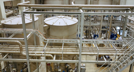
(b)

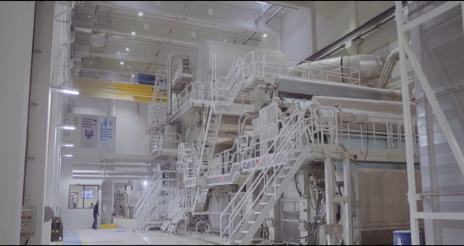
(c)

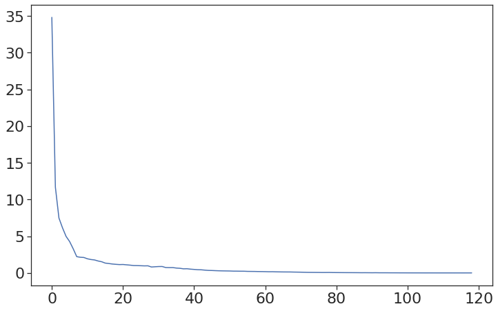
(d)

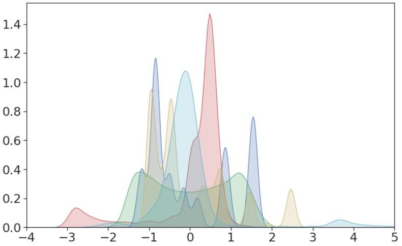
(e)

Figure 1: Panels (a)-(c) show three phases of the production process of the A.Celli tissue machine. Panel (d) shows the eigenvalues of the correlation matrix of the 119 variables considered in our case study. Panel (e) shows the densities of 5 among these variables after standardization.

${\mathit{SAnD}}{}$ was developed with the industrial partner A.Celli, leader in the supply of machinery and technologies for the paper and nonwoven products industry. The company provided data from a tissue paper machine, which comprised 217 variables measured every second for about 19 hours. This is a complex production line with several phases, three of which are depicted in Figure 1 (a)-(c), that can tackle different products. We focused on a specific product, which reduced the variables to consider to 119. The collaboration aimed to develop a methodology to detect anomalies in the production process of tissue machines, with two key requirements, namely: (R1) enable quick and accurate identification of the time intervals in which anomalies occur; (R2) provide information on patterns and variables involved in the anomalies, to help domain experts decipher their causes.

We note that the data at our disposal contained exclusively intervals assessed as anomaly-free by the domain experts. In other words, no known instances of anomalies were provided, so we could not resort to supervised methods, which need to be trained on data comprising both anomalies and anomaly-free observations. The procedure we developed classifies as semi-supervised based on the definition in Schmidl et al. (2022); we do not exploit anomaly labels in the training data, but rather data concerning only normal, anomaly-free behavior.

In addition to R1 and R2, the considered scenario required that we focus on long-lived anomalies, i.e., anomalies lasting for minutes (over observations taken per second), since in this domain short-lived anomalies are likely due to sensor noise. Note that, for each long-lived anomaly, it suffices to flag just one observation within its time interval to alert an expert who will then investigate the issue. In other words, long-lived anomalies can be detected through at least one true positive within their time-span. Finally, we wanted our procedure to be general, and thus easily exportable to additional (industrial) domains.

The last decade has seen the development of a multitude of sophisticated semi-supervised methods based, e.g., on deep learning or statistical learning techniques, which should be able to tackle R1-2 by leveraging complex patterns in the data without the introduction of strong assumptions (see Choi et al. 2021; Blázquez-García et al. 2021; Schmidl et al. 2022 for recent reviews). However, the comprehensive comparison in Schmidl et al. (2022) demonstrates that no single method offers the best performance across different scenarios.

In contrast, ${\mathit{SAnD}}{}$ exploits the Mahalanobis distance (Mahalanobis, 1936) evaluated on the training data as a means to identify anomalies. This is an extremely simple approach, which requires only estimates of location and covariation from the training data. However, data from industrial processes do pose technical challenges (TC) also for the use of such a straightforward approach. The first (TC1) is multicollinearity. Figure 1 (d) shows the eigenvalues of the correlation matrix of the 119 variables generated by the A.Celli tissue machine; the smallest are close to 0, indicating strong multicollinearity. This is a problem, since the Mahalanobis distance requires the covariance matrix to be invertible. The second technical challenge (TC2) concerns the distribution of the data. Figure 1 (e) shows the densities of 5 variables randomly selected among the 119. Clearly, even under anomaly-free conditions, the distributions are far from Gaussian, or other typical forms, e.g., used to represent skewed data (Rousseeuw and van Zomeren, 1990; Hubert and Van der Veeken, 2008; Tiku et al., 2010; Todeschini et al., 2013; Cabana et al., 2019). When one can postulate that anomaly-free data follow a Gaussian or other known distributions, it is possible to derive a distribution for the Mahalanobis distance and, based on such distribution, to define a threshold for the indentification of anomalies (Rousseeuw and Leroy, 2005; Maronna et al., 2019). When distributional assumptions are unsuitable, one must resort to different approaches to define an appropriate threshold.

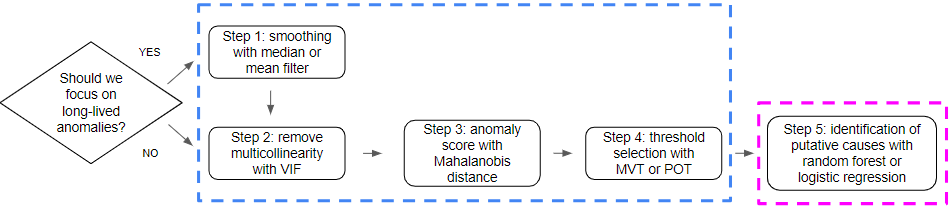
Figure 2: Flow chart of the proposed procedure. The dashed blue line shows the steps used to tackle R1, while the dashed purple line shows the step used to tackle R2.

Our procedure, which attempts to address all the challenges and considerations raised thus far, consists of the 5 steps depicted in Figure 2. We start with an anomaly-free dataset, which represents the training set for our procedure. The first step consists of smoothing the data through a median or mean filter, as to remove short-lived anomalies; this step is optional, and should be applied only if the focus is on long-lived anomalies. The second step mitigates multicollinearity removing variables based on their variance inflation factors (Craney and Surles, 2002). In the third step, we compute the Mahalanobis distances for all points in the training set. The fourth step provides a threshold for the identification of anomalies. If no distributional assumptions are possible, we use the maximum value of the Mahalanobis distances in the training set (MVT), or the value produced by a Peaks-Over-Threshold (POT) analysis of the right tail of such distances (Balkema and De Haan, 1974; Pickands III, 1975). The data in the test set undergoes smoothing, as the training data. A Mahlanobis distance is produced for each test data point, and a (binary) anomaly prediction is produced based on whether its distance is above threshold. Finally, the fifth step uses feature importance techniques offered by random forest (Breiman, 2001) or logistic regression (James et al. 2013, ch. 4) to analyze anomalies predicted in the test set, unveiling patterns and pinpointing relevant variables, as to decipher their putative causes.

In our comparisons, we employ common performance metrics such as the Matthews correlation coefficient (MCC) (Chicco and Jurman, 2020), F1, recall, and precision. We also assess computational cost through runtime analyses. Additionally, we showcase the effectiveness of our procedure on the A.Celli case study which motivated its development.

The article is organized as follows. Section 2 focussz on the properties of the Mahalanobis distance. Section 3 details ${\mathit{SAnD}}$. Section 4 demonstrates its performance through a comprehensive validation on methods and datasets from Schmidl et al. (2022). Section 5 relates its feature importance results to the causes of the anomalies. Finally, Section 6 demonstrates ${\mathit{SAnD}}{}$ on the case study, and Section 7 provides final remarks. Replicability material for Sections 4 and 5 is available at https://doi.org/10.5281/zenodo.11032650.

2 Some background on the Mahalanobis distance

The Mahalanobis distance (Mahalanobis, 1936) is one of the key statistical tools employed by ${\mathit{SAnD}}$. It has low computational requirements and high interpretability, as it allows one to quantify how much an observation deviates from “behavior under normal conditions” through straightforward estimation of the mean vector and covariance matrix of the training data. Here we focus on aspects that make it suitable for anomaly detection in semi-supervised contexts, while we discuss other background material in Supplement B.

Let $\mathbf{X}_{A}=\mathopen{}\mathclose{{}\left\{\mathbf{x}_{t}}\right\}_{t=1}^{T_{A}}$ denote an $n\times T_{A}$ rectangular array of observations on $n$ stationary time series (i.e., time series with finite variance, see Choi et al. 2021) with $T_{A}$ observations for each series. In practice, $\mathbf{X}_{A}$ is provided by a domain expert to denote the behavior of the process under normal conditions. Given a new rectangular array $\mathbf{X}_{B}=\mathopen{}\mathclose{{}\left\{\mathbf{x}_{t}}\right\}_{t=T_{A}+1}^{T}$ of dimension $n\times T_{B}$, where $T_{B}=T-T_{A}$, we focus on the question: How distant is each point in $\mathbf{X}_{B}$ from the behavior captured by $\mathbf{X}_{A}$? The Mahalanobis distance is a common approach to answer this. Let $\widehat{\boldsymbol{\mu}}_{A}$and $\widehat{\boldsymbol{\Sigma}}_{A}$ be the mean vector and covariance matrix estimated on $\mathbf{X}_{A}$. For a given $n$-dimensional observation in the test set, say $\mathbf{x}_{\tilde{t}}=(x_{1,\tilde{t}},\dots,x_{n,\tilde{t}})^{\prime}$ with $T_{A}\!+\!1\leq\tilde{t}\leq T$, the Mahalanobis distance from the training set is defined as

$$MD_{\tilde{t}}=\sqrt{(\mathbf{x}_{\tilde{t}}-\widehat{\boldsymbol{\mu}}_{A})^{\prime}\ \widehat{\boldsymbol{\Sigma}}_{A}^{-1}\ (\mathbf{x}_{\tilde{t}}-\widehat{\boldsymbol{\mu}}_{A})}\ \ .$$ (1)

$MD_{\tilde{t}}$ measures how far $\mathbf{x}_{\tilde{t}}$ is from the center of the training data in an inner product that is shaped by its inverse covariance – so directions of higher (co)variation matter less in assessing departure from the center.

As mentioned in the Introduction, industrial processes can have large operational variability, as well as substantial collinearities, under normal conditions. The next assumption is fundamental to apply semi-supervised anomaly detection methods in this context.

Assumption 1:

$\mathbf{X}_{A}$ is representative of the operational variability of the process under normal conditions.

We can expect $\mathbf{A1}$ to hold for large $T_{A}$. The importance of $\mathbf{A1}$ lies in the fact that we can identify $p\leq n$ eigenvectors of $\widehat{\boldsymbol{\Sigma}}_{A}$ whose span approximates the linear sub-space to which the normal conditions belong. In particular, let $\mathbf{v}_{1},\dots,\mathbf{v}_{n}$ be the eigenvectors of $\widehat{\boldsymbol{\Sigma}}_{A}$ ordered based on the corresponding eigenvalues $\lambda_{1}\geq\dots\geq\lambda_{n}$, and let $p$ be the smallest integer such that $\frac{\sum_{i=1}^{p}\lambda_{i}}{\sum_{i=1}^{n}\lambda_{i}}>\alpha$, where $\alpha\in[0,1]$ is a threshold value (e.g., 0.99). This means that the first $p$ principal components explain $100\times\alpha$% of the variability of $\mathbf{X}_{A}$. Under $\mathbf{A1}$, such components explain most of the operational variability of the process under normal conditions, while the Mahalanobis distance will increase more steeply for an observation varying in the direction of the remaining $n-p$ components (Deraemaeker and Worden, 2018). The following proposition formalizes this reasoning.

Proposition 1:

Under Assumption $\mathbf{A1}$, let $\sum_{i=1}^{p}\lambda_{i}$ be the sum of the $p$ largest eigenvalues, associated with the eigenvectors that explain $100\times\alpha\%$ of the variability of $\mathbf{X}_{A}$. If $\sum_{i=1}^{p}\lambda_{i}\rightarrow\sum_{i=1}^{n}\lambda_{i}$ (i.e., $\alpha\rightarrow\ 1^{-}$), then $MD_{\tilde{t}}$ tends to the Mahalanobis distance of $\mathbf{x}_{\tilde{t}}$ projected on the space described by the remaining $n-p$ components.

Proof: See Supplement A.

Proposition 1 shows that by including all operational variability (the variables measured in all possible environmental conditions) in computing the covariance matrix $\widehat{\mathbf{\Sigma}}_{A}$, the Mahalanobis distance increases as $\mathbf{x}_{\tilde{t}}$ moves away from the normal conditions of the process. This property justifies its use in anomaly detection. However, as discussed in the Introduction, some technical challenges (TC1-2) complicate such use in the considered domain. Section 3 shows how some of the step included in ${\mathit{SAnD}}{}$ solve these issues.

3 The 5-step SAnD procedure

In this section, we present our procedure to detect anomalies in industrial contexts. ${\mathit{SAnD}}{}$ combines five main elements; namely: smoothing filters, variance inflation factors, Mahalanobis distance, threshold selection procedures, and feature importance techniques. Let $\mathbf{X}_{A}$ and $\mathbf{X}_{B}$ be rectangular arrays on $n$ variables as in Section 2. For the $n\times T$ matrix $\mathbf{X}=(\mathbf{X}_{A},\mathbf{X}_{B})$, the proposed procedure comprises the following steps.

Step 1 - Smoothing (optional).

If the problem at hand concerns only long-lived anomalies, we smooth each of the time series with a filter based on location measures (mean, or median for robustness) computed on a moving window of given size, say $h$. This replaces each of the $T$-dimensional vectors $\mathbf{x}_{i}$, $i=1,\dots,n$ with a corresponding $(T-(h-1))$-vector of smoothed values $\mathbf{w}_{i}$. To simplify notation, we indicate with $\ddot{T}=T-2(h-1)$, $\ddot{T}_{A}=T_{A}-(h-1)$ and $\ddot{T}_{B}=T_{B}-(h-1)$ the sizes of the smoothed vectors. Therefore, we replace the $n\times T$ matrix $\mathbf{X}=(\mathbf{X}_{A},\mathbf{X}_{B})$ with the $n\times\ddot{T}$ matrix $\mathbf{W}=(\mathbf{W}_{A},\mathbf{W}_{B})$, where $\mathbf{W}_{A}$ ($n\times\ddot{T}_{A}$) comprises smoothed values in normal conditions, and $\mathbf{W}_{B}$ ($n\times\ddot{T}_{B}$) smoothed values among which we want to detect anomalies.

Smoothing allows us to mitigate short-lived anomalies that would be considered as sensor noise by domain experts, and thus to avoid false positives. Domain experts will be in a position to select between mean filtering or the more robust median one, and to specify an appropriate window size $h$ for given applications. In the experiments in the following Sections, we rely on median filtering and we consider $h=1$ (no smoothing) and $h=10$.

Step 2 - Removing multicollinearity (to address TC1).

We use Variance Inflation Factors, VIF (Craney and Surles, 2002), to quantify multicollinearity among the variables in the training data $\mathbf{W}_{A}$ (or $\mathbf{X}_{A}$ if we omit the smoothing) and iteratively remove some of them. We first subtract from the entries of each $\mathbf{w}_{Ai}$ its mean $\bar{w}_{Ai}=\ddot{T}_{A}^{-1}\sum_{t=1}^{\ddot{T}_{A}}w_{it}$, switching to $\mathbf{d}_{Ai}=\mathbf{w}_{Ai}-\bar{w}_{Ai}\mathbf{1}$, and form the centered matrix $\mathbf{D}_{A}$ (centering is not necessary here; however, popular statistical software packages require it in order to compute VIFs ignoring intercepts). Next, we regress each variable in $\mathbf{D}_{A}$ against all others, compute the coefficients of determination from such regressions, say $R_{i}^{2}$, and thus the VIFs, which are given by VIF${}_{i}\!=\!1/(1-R_{i}^{2})$, $i\!=\!1,\ldots n$. We remove the variable with largest VIF, re-run the regressions and recompute the VIFs, remove again the variable with largest VIF, et cetera – until the largest VIF is less than 5, a benchmark commonly used in the literature (James et al. 2013, ch. 3.3). This leaves us with a set of $m$ $(\leq n)$ variables with at most mild multicollinearity. We indicate the reduced, centered training data matrix as $\widetilde{\mathbf{D}}_{A}$.

Mitigating multicollinearity is critical because the Mahalanobis distance utilizes the inverse of the covariance matrix estimated on the data (see Equation (1)); the strong linear associations which exist in our case study (see Figure 1 (d)) and many other applications may prevent such inversion. The covariance matrix $\boldsymbol{\tilde{\Sigma}}_{A}=\ddot{T}_{A}^{-1}\widetilde{\mathbf{D}}_{A}\widetilde{\mathbf{D}}_{A}^{\prime}$ relative to the $m$ non-multicollinear variables will not present any invertibility issues.

Step 3 - Computing anomaly scores.

We start by processing the test data $\mathbf{W}_{B}$. First, we center it with the means computed on the training data, switching to $\mathbf{d}_{Bi}=\mathbf{w}_{Bi}-\bar{w}_{Ai}\mathbf{1}$ and forming the centered matrix $\mathbf{D}_{B}$. Next, we reduce such matrix eliminating the same variables that were eliminated from the training data in Step 2; we indicate the reduced, centered test data matrix as $\widetilde{\mathbf{D}}_{B}$. Finally, we calculate Mahalanobis distances for the full dataset $\widetilde{\mathbf{D}}=(\widetilde{\mathbf{D}}_{A},\widetilde{\mathbf{D}}_{B})$ (that is, for both training and test observations) using the training covariance matrix; in symbols $MD_{t}=\sqrt{\widetilde{\mathbf{d}}_{t}^{\prime}\boldsymbol{\tilde{\Sigma}}_{A}^{-1}\widetilde{\mathbf{d}}_{t}}$, $t=1,\dots,\ddot{T}$. We indicate with $\boldsymbol{MD}_{T}$, $\boldsymbol{MD}_{A}$ and $\boldsymbol{MD}_{B}$, respectively, the $T$, $\ddot{T}_{A}$ and $\ddot{T}_{B}$-dimensional vectors of anomaly scores for the full dataset, the training set and the test set.

Step 4 - Threshold selection (to address TC2).

We use $\boldsymbol{MD}_{A}$ to select a threshold $k$ beyond which an observation in $\boldsymbol{MD}_{B}$ is flagged as an anomaly. Note that if we can assume the variables retained in Step 2 to be distributed as an $m$-variate Gaussian under normal conditions, the quadratic form expressing the Mahalanobis distance will be distributed as a chi-square with $m$ degrees of freedom (Penny, 1996). Thus, setting the threshold as a quantile of such chi-square, say $k=\chi^{2}_{m}(1-\alpha)$, would guarantee a p-value of $\alpha$ when flagging anomalies (one-sided rejections). However, unfortunately, the variables in our reference domain are far from Gaussian (see Figure 1 (e)). We therefore resort to other approaches to select the threshold $k$; namely, the Maximum Value in the Training sample (MVT) and Peaks-Over-Threshold (POT) approaches. In the former, the threshold is simply set at the largest value in $\boldsymbol{MD}_{A}$, using, in a way, an empirical p-value of 0 when flagging anomalies. In the latter, we fit a generalized Pareto distribution (Siffer et al., 2017) to the peaks in the training set, i.e., the elements of $\boldsymbol{MD}_{A}$ above a given percentile (we fix the 99th one). Using a known formula (see Supplement B.1), we thus obtain a threshold $k$ that depends on the peaks, on the parameters of the fitted distribution, and on a chosen probability (we fix 0.001) for a peak to be an anomaly, or an extreme event in POT terminology.

Once the threshold $k$ is fixed, we compare each observation $MD_{\tilde{t}}$ in $\boldsymbol{MD}_{B}$ with $k$, and generate a binary vector $\widehat{\mathbf{y}}=(\widehat{y}_{1},\dots,\widehat{y}_{\ddot{T}_{B}})$, with $\widehat{y}_{\tilde{t}}=1$ if $MD_{\tilde{t}}>k$ and 0 otherwise.

Step 5 - Identifying variables involved in anomalies (to address R2).

After detecting anomalies, we try to associate them to specific variables – as to aid domain experts in the investigation of putative causes. We do so by training supervised methods equipped with feature importance techniques, using the detected anomalies in $\widehat{\mathbf{y}}$ as prediction targets. In more detail, we fit a prediction model on each time interval of interest (i.e., each interval from the test set corresponding to a detected long-lived anomaly), which we combine with arbitrarily selected anomaly-free observations (in our experiments in Section 5 we use observations from the final portion of the training set, while in Section 6 we use anomaly-free observations from the same interval containing anomalies). We use two well-known prediction models; namely, random forest (Breiman, 2001) and logistic regression (James et al. 2013, ch. 4). Feature importance is evaluated through the Gini Index for the former (see Supplement B.2 and James et al. 2013 ch. 8), and through the Relative Contribution to Deviance Explained (RCDE) for the latter (see Supplement B.3 and Tripodi et al. 2020).

4 Evaluation of performance and runtime

We evaluate our procedure in terms of performance and computational cost by comparing it with several state-of-the-art semi-supervised anomaly detection techniques on multiple public datasets from the anomaly detection literature. For the selection of techniques and datasets to employ in our comparison, we rely on the recent, broad survey by Schmidl et al. (2022). The survey comprised eleven semi-supervised techniques, of which we consider nine; namely, LSTM-AD (Malhotra et al., 2015), HealthESN (Chen et al., 2020), Telemanom (Kyle et al., 2018), Random Black Forest (Schmidl et al., 2022), EncDec-AD (Malhotra et al., 2016), DEEPAnT (Munir et al., 2018), Omnianomaly (Su et al., 2019), Robust-PCA (Paffenroth et al., 2018), and Hybrid-KNN (Song et al., 2017) – all run using settings and implementations provided in Schmidl et al. (2022) and in its replicability material at https://github.com/TimeEval/TimeEval-algorithms. We omit LaserDBN (Ogbechie et al., 2017) and TAnoGan (Bashar and Nayak, 2020) due to implementation issues, but these were among the bottom ranking in the evaluation by Schmidl et al. (2022).

We run ${\mathit{SAnD}}$ with both $h=1$ (no smoothing, ${\mathit{SAnD}}_{1}$) and $h=10$ (smoothing, ${\mathit{SAnD}}_{10}$). Since most of the procedures, including ours, provide an anomaly score to be compared against a threshold, we homogenize the comparison using the same threshold selection methods, namely MVT and POT, for all procedures. The only exception is Hybrid-KNN, which returns the probability that an observation is an anomaly. Here we present results obtained setting a threshold of $0.8$ on such probability; higher thresholds (e.g., $0.9$ and $0.99$) do not noticeably change the performance of Hybrid-KNN (see Supplement D).

The survey by Schmidl et al. (2022) considered 24 collections of public datasets from the anomaly detection literature. Only 2 of these collections contain non-synthetic multivariate time series and comprise anomaly-free data as required by semi-supervised methods; namely, the Server Machine Datasets, SMD (Su et al., 2019), and the Exathlon (Filonov et al., 2016). From each of these two collections we randomly selected 4 datasets that contain long-lived anomalies. SMD, one of the largest public data repositories available for anomaly detection in multivariate time-series, contains 5-week-long datasets collected per minute by a large internet company on 28 different machines. It comprises one dataset per machine, each with 38 variables. Exathlon contains 39 datasets with about 23 variables on average. It has been used in the context of industrial fault detection, a specific type of anomaly. For both collections, the training sets are anomaly-free, while the test sets are not, and have labels to denote anomalies. The datasets from SMD contain both short- and long-lived anomalies, while the ones from Exathlon contain only long-lived anomalies. Table 1 shows some statistics on the datasets.

Collection	Avg. Size	Avg. Dim.	Avg. Cont.
SMD	54 827	38.00	4.04%
Exathlon	94 186	23.25	7.32%

Table 1: Some statistics on the 8 datasets used in our comparison. We consider 4 datasets from each of two collections, listing averages for: number of observations (Avg. Size), number of variables (Avg. Dim.), and contamination (Avg. Cont.) – i.e., the percentage of test observations labeled as anomalies.

In terms of performance metrics, we use various well-known indicators of accuracy in anomaly detection; namely: precision, $\mathit{Prec}=TP/(TP+FP)$; recall, $\mathit{Recall}=TP/(TP+FN)$; the harmonic mean of the two, or F1 score, $F1=2TP/(2TP+FP+FN)$; and the Matthews Correlation Coefficient (Chicco and Jurman, 2020)

$$MCC=\frac{TP\times TN-FP\times FN}{\sqrt{(TP+FP)\times(TP+FN)\times(TN+FP)\times(TN+FN)}}$$

which, ranging in $[-1,1]$, measures the agreement between true and detected anomalies. All these metrics combine, in intuitive and effective ways, counts of true positives (TP), true negatives (TN), false positives (FP) and false negatives (FN). Notably though, since they consider individual anomalous observations, they might not be suited to evaluate methods when the focus is on long-lived anomalies. This is because they do not tell us whether long-lived anomalies were flagged by detecting at least one anomaly within them. To capture this, we use an additional metric named RIC (Ratio of Identified Clusters), where a “cluster”, i.e., a long-lived anomaly, is counted as identified if at least one observation within its time frame is detected as an anomaly (see Supplement E).

Method	Prec	Recall	F1	MCC	RIC	%No Anom.
MVT
LSTM-AD	0.667 (0.37)	0.124 (0.20)	0.104 (0.15)	0.168 (0.15)	0.309 (0.44)	62.5%
HealthESN	0.582 (0.39)	0.511(0.51)	0.211 (0.16)	0.209 (0.13)	0.928(0.14)	0.0%
Telemanom	0.713 (0.17)	0.054 (0.08)	0.104 (0.14)	0.148 (0.21)	0.229 (0.37)	62.5%
RBForest	0.998 (0.01)	0.014 (0.02)	0.030 (0.04)	0.140 (0.07)	0.365 (0.45)	50.0%
EncDec-AD	0.370 (0.52)	0.003 (0.01)	0.009 (0.02)	-0.007 (0.10)	0.025 (0.07)	50.0%
DeepAnT	0.827 (0.23)	0.100 (0.16)	0.140 (0.22)	0.278 (0.22)	0.246 (0.27)	62.5%
OmniAnomaly	0.907 (0.09)	0.093 (0.14)	0.152 (0.22)	0.318 (0.26)	0.272 (0.38)	62.5%
RobustPCA	1.000(0.00)	0.033 (0.05)	0.061 (0.08)	0.222 (0.11)	0.192 (0.28)	50.0%
${\mathit{SAnD}}_{1}$	1.000(0.00)	0.304 (0.43)	0.342 (0.44)	0.427 (0.43)	0.813 (0.37)	12.5%
${\mathit{SAnD}}_{10}$	0.872 (0.31)	0.491 (0.43)	0.650(0.41)	0.630(0.45)	0.823 (0.35)	12.5%
POT
LSTM-AD	0.603 (0.37)	0.155 (0.25)	0.117 (0.14)	0.160 (0.15)	0.376 (0.47)	62.5%
HealthESN	0.529 (0.37)	0.496 (0.47)	0.244 (0.12)	0.219 (0.15)	1.000(0.00)	0.0%
Telemanom	0.852 (0.17)	0.460 (0.41)	0.522 (0.38)	0.482 (0.41)	0.638 (0.43)	16.67%
RBForest	0.614 (0.28)	0.533 (0.38)	0.421 (0.28)	0.369 (0.31)	1.000(0.00)	0.0%
EncDec-AD	0.573 (0.52)	0.018 (0.02)	0.038 (0.04)	0.035 (0.14)	0.112 (0.13)	25.0%
DeepAnT	0.715 (0.32)	0.266 (0.32)	0.140 (0.34)	0.380 (0.37)	0.469 (0.51)	50.0%
OmniAnomaly	0.883 (0.12)	0.164 (0.17)	0.315 (0.23)	0.320 (0.26)	0.436 (0.41)	40.0%
RobustPCA	0.890 (0.09)	0.061 (0.08)	0.110 (0.15)	0.250 (0.14)	0.475 (0.51)	50.0%
${\mathit{SAnD}}_{1}$	0.901(0.17)	0.585 (0.44)	0.635 (0.39)	0.624 (0.41)	1.000(0.00)	0.0%
${\mathit{SAnD}}_{10}$	0.841 (0.25)	0.673(0.42)	0.666(0.38)	0.645(0.40)	0.844 (0.35)	12.5%
$\Pr>0.8$
Hybrid KNN	0.143 (0.31)	0.312 (0.43)	0.309 (0.22)	0.959 (0.22)	0.625 (0.21)	0.0%

Table 2: Performance evaluation for each method and threshold selection procedure. In the POT case, HealthESN and RBForest were run on 7 datasets, Telemanom on 6, and Omnianomaly on 5 because the parameters of the generalized Pareto distribution could not be calculated on some of the datasets (see Supplement B.1). For the Exathlon collection, EncDec-AD failed to calculate anomaly scores. In addition to the performance metrics, which are averaged over the datasets (in parenthesis the standard deviations), the last column provides the percentage of datasets out of the considered ones where no long-lived anomalies were identified (%No Anom.). The best performance for each metric and thresholding procedure is in bold.

Table 2 reports, for each method and threshold selection procedure, all performance metrics averaged over the datasets, along with the percentage of datasets where no long-lived anomalies were identified (%No Anom.). ${\mathit{SAnD}}$ shows consistently high performance. In particular, it always has the best performance with POT, and either the best or second-best with MVT. Smoothing in ${\mathit{SAnD}}$ tends to have a positive impact on F1 and MCC, while %No Anom. might worsen due to the loss of anomalies in the datasets from SMD.

We now focus on performance in detecting long-lived anomalies. For each dataset, we compute the arithmetic mean between Prec (which controls false positives) and RIC (which targets specifically long-lived anomalies), restricting attention to the portion of the test set that contains long-lived anomalies (see Supplement F for more details). In Figure 3, for each method and thresholding procedure combination, the average of this summary across the considered datasets is plotted against the average runtime of the method – computed as the logarithm of the seconds needed to compute the anomaly scores. In general, we see that POT improves the identification of long-lived anomalies (see also $RIC$ results in Table 2; the improvement is most marked for the Telemanom method). Most notably though, with both thresholding procedures and with and without smoothing, ${\mathit{SAnD}}$ is located in the upper left corner of Figure 3, representing the best-performing method with the least runtime. In Supplement C we report runtimes separately for training and test sets. In summary, our comparison demonstrates that ${\mathit{SAnD}}$ outperforms competitors in both anomaly detection accuracy and runtime, addressing R1.

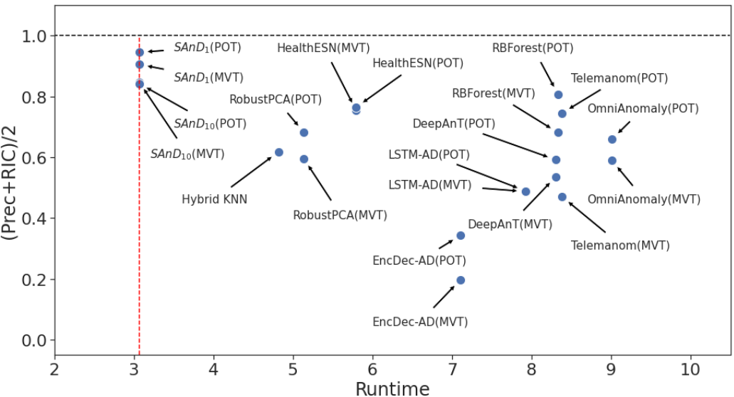
Figure 3: Performance of each method and threshold procedure, focusing on long-lived anomalies (y-axis), vs runtime expressed as logarithms of seconds needed to compute anomaly scores (x-axis). Performances and runtimes are averaged across the considered datasets. Hybrid KNN uses the threshold $\Pr>0.8$.

5 Evaluation of feature importance

The last step of ${\mathit{SAnD}}$ uses random forest or logistic regression to associate detected anomalies to specific variables. Here, we try and evaluate whether and how feature importance assessed by these prediction models can shed light on the putative causes of anomalies. The datasets in SMD comprise information on the variables that caused each anomaly. We thus use the first dataset from SMD for our evaluation, focusing in particular on 5 anomalies, among the 8 within it, that are long-lived (they last several minutes, see Supplement F).

The first four steps of ${\mathit{SAnD}}$ run with $h=1$ and POT detect all these long-lived anomalies. We run step 5 by training random forest and logistic regression for each such anomaly, using 1 000 observations from the test set containing the anomaly, and 1 000 additional anomaly-free observations from the training set (see Supplement F for details).

Anom.	Causes	Ranked by RF, $h=1$	Ranked by LR, $h=1$
1	1,9,10,12,13,14,15	10,12,13,9,15,14,1	10,15,9,6,13,2,1
2	1,2,3,4,6,7,9,10,11,12,	34,20,35,1,36,13,10,28,29,31,	10,1,6,4,9,15,23,2,11,36,
	13,14,15,16,19,20,21,22,24,25,	12,22,2,21,3,33,25,19,15,14,	35,3,32,16,21,20,19,13,34,14,
	26,27,28,29,30,31,32,33,34,35,36	6,26,4,32,23,16,7,11,24,30	24,31,26,29,33,25,22,30,28,12,7
3	1,2,9,10,12,13,14,15	10,12,13,20,1,9,28,22	10,15,1,13,34,29,9,14
4	1,2,3,4,9,10,11,12,13,14,15,16,25,28	10,12,13,7,6,20,34,9,29,36,25,28,30,15	10,6,29,14,11,23,16,13,34,33,2,9,1,15
5	1,9,10,12,13,14,15	10,13,12,9,15,14,23	10,9,33,15,23,24,26

Table 3: Variables labeled as causes in the dataset vs variables ranked as important for the anomalies by Random Forest (RF) and logistic regression (LR). We mark such important variables in bold if they are among the labeled causes, and in red if they are not. With very few exceptions (e.g., anomaly 4, LR) the top portion of the rankings is occupied by variables labeled as causes.

Table 3 summarizes results. The real causes indicated by the dataset description are reported in the section labeled Causes; variables here are arbitrarily numbered based on the column order in the data set, and listed based on such numbers – but SMD does not provide information on the importance of the causes; that is, the variables are not ranked. Sections Ranked by RF and Ranked by LR report the variables identified as most relevant using random forest and logistic regression, respectively, ranked by (decreasing) importance (see Supplement G). For each anomaly $a$, we include the $v(a)$ most important variables, $v(a)$ being the number of variables indicated as causes in the dataset description. We see that the results of step 5 are indeed coherent with the causes as given in the dataset; 82.1% and 79.1% of the variables identified by our procedure using RF and LR, respectively, are among such causes. This demonstrates how ${\mathit{SAnD}}$ can effectively address R2.

6 Case study

Next, we demonstrate the effectiveness of ${\mathit{SAnD}}{}$ on an industrial case study involving a tissue machine of the A.Celli company. This application was performed in close collaboration with domain experts who validated its results.

The data consisted of 70 000 observations collected per second on 217 variables. We used the first 60 000 for training, and the last 10 000 for testing. In the considered time interval, the machine handled only one type of product, allowing us to restrict attention to 119 variables deemed relevant for this one product. For the smoothing in step 1 of ${\mathit{SAnD}}{}$, we considered two window sizes; $h=1,10$. For the feature importance assessment in step 5, we focused on random forest ($RF$ performed slightly better than $LR$ in Section 5).

We start from the analysis with no smoothing ($h=1$). In step 2, because of high multicollinearity in our case study, VIFs reduced the variables from 119 to 60. In step 3 we computed the anomaly scores, and in step 4 we thresholded them with MVT to detect the four anomalies shown in Figure 4 (a)-(b). Zooming in (Figure 4 (b)), we can see that three are short-lived and one is long-lived. However, given that they are very close, the domain experts interpreted the ‘cluster’ of four detected anomalies as a single long-lived anomaly. Therefore, in step 5 we investigated the putative causes of the cluster of detected anomalies as a whole. We did this by training a random forest on the entire interval (2000 observations) shown in Figure 4 (b). Differently from Section 5, here we do not need to add anomaly-free observations from the training sample, because such interval contains plenty of anomaly-free observations. The domain experts deemed the top $v=5$ variables as sufficient and relevant for interpreting the causes of the anomalies. These are: WERecirculationFanPower, DERecirculationFanPower (two energy expenditure variables for the fans that manage humidity and the drying process of the sheet), MCC1PowerConsumption (power consumption of the electrical distribution panel), DEGasConsumption (gas consumption of the drying process), V6-Speed (speed of a fan used to dry the sheet). Figure 4 (c), which depicts the time series of these 5 variables, clearly suggests the presence of a long-lived anomaly. Indeed, the domain experts were able to validate our findings as an actual process anomaly caused by overheating of the system during the paper drying phase.

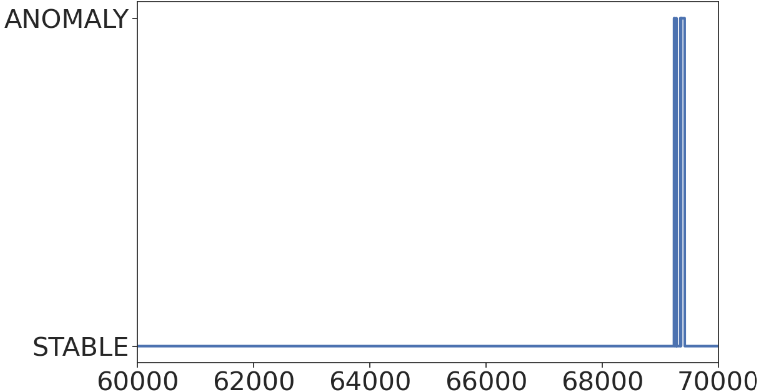
(a)

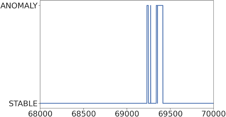
(b)

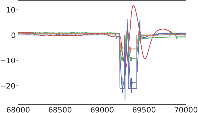
(c)

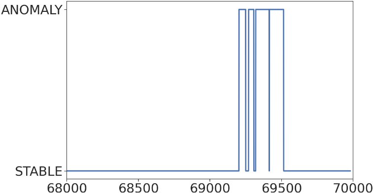
(d)

Figure 4: Case study results using MVT thresholding. Plot (a) shows anomalies detected in the test set by ${\mathit{SAnD}}_{1}$ (no smoothing, $h=1$). Plot (b) highlights such anomalies zooming in on the last 2 000 observations. Plot (c) shows the time series of the 5 most important variables as identified by a Random Forest. Plot (d) is the same as Plot (b), but for ${\mathit{SAnD}}_{10}$ (smoothing with $h=10$).

Running ${\mathit{SAnD}}$ with smoothing ($h=10$) lends further support to the existence of one long-lived anomaly. The VIFs in step 2 leads to the same 60 variables obtained without smoothing. Thresholding the resulting anomaly scores, again with MVT, detects one, essentially uninterrupted long-lived anomaly in the same time interval (Figure 4 (d)). A random forest, trained again on the 2 000 observations in Figure 4 (b) but using smoothed data, ranks as top 5 variables BRConsistency (pulp consistency setpoint), WERecirculationFanPower, MCC1PowerConsumption, Thermocompressor (sensor on drying phase), and SF-Refiner-Outlet-Pressure (outlet pressure of the SF refiner). While three of these variables differ from those for $h=1$, according to the domain experts they point to the same cause, i.e., overheating during the paper drying phase.

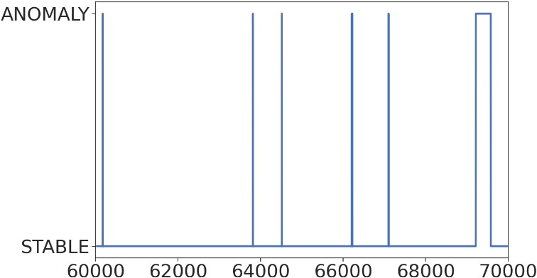
(a)

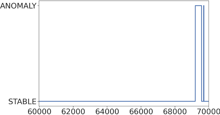
(b)

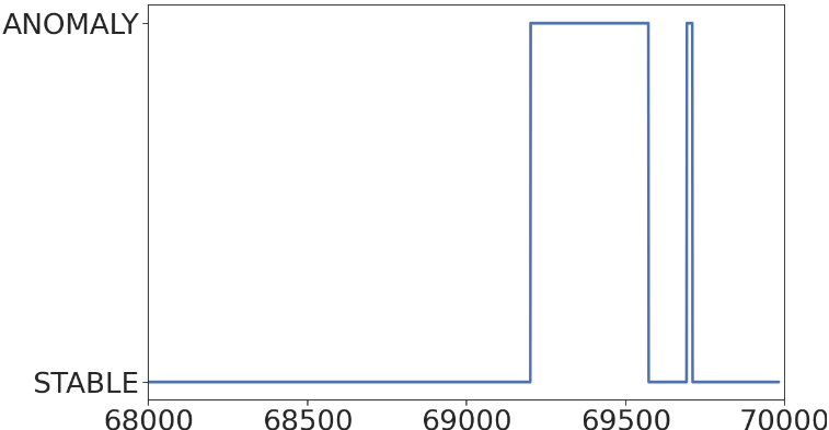
(c)

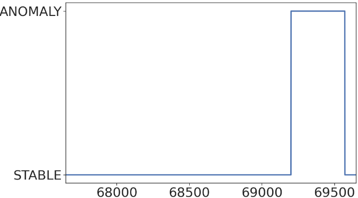
(d)

Figure 5: Results in the case of POT. Plots (a) and (b) show the anomalies detected in the test set by ${\mathit{SAnD}}_{1}$ and ${\mathit{SAnD}}_{10}$, respectively. Plot (c) highlights the anomalies detected by ${\mathit{SAnD}}_{10}$ by showing the last 2 000 observations only. Plot (d) highlights the long-lived anomaly detected by ${\mathit{SAnD}}_{10}$.

Next, we switched from MVT to POT thresholding. Figure 5 (a) displays results without smoothing ($h=1$). POT detects many more anomalies than MVT (Figure 4 (a)), and especially many short-lived ones attributed by domain experts to sensor noise. Figures 5 (b)-(c) display results with smoothing ($h=10$), which makes ${\mathit{SAnD}}$ more suited to long-term anomalies; ${\mathit{SAnD}}_{10}$ detects 1 long-lived and 1 short-lived anomaly, discarding other sensor noise detected by ${\mathit{SAnD}}_{1}$. The domain experts deemed the long-lived anomaly to be the same as that in Figure 4 (d). Indeed, the time interval involved is almost identical. Training a random forest on the 2 000 observations in Figure 5 (d) we find that 3 of the 5 top ranked variables are shared with those identified by ${\mathit{SAnD}}_{10}$ with MVT thresholding; namely, BRConsistency, WERecirculationFanPower and MCC1PowerConsumption. The other top variables are SheetON (if paper passes from the last roll to the winder), and DERecirculationFanPower (also identified by ${\mathit{SAnD}}_{1}$ with MVT). According to the domain experts, also this new selection of variables pointed to system overheating. Step 5 run for the short-lived anomaly in Figure 5 (c) produces a different ranking of the variables, but still a clear connection to system overheating (see Supplement H).

This analysis exemplifies an important aspect of anomaly detection: the real cause underlying an anomaly might not be directly expressed by the observed variables, and domain knowledge is required to reconstruct causes. In our case study, the variable “system overheating” does not exist as such. However, the variables selected by step 5 of ${\mathit{SAnD}}$ with various specifications (with or without smoothing, with different thresholding) all point to the slowing and cooling of the production system, allowing our industrial partners to identify system overheating as the underlying cause.

7 Concluding remarks

We introduced ${\mathit{SAnD}}$, a procedure based on simple and well-known statistical tools to detect anomalies in industrial processes characterized by multicollinear time series with unknown distribution. Experiments show that ${\mathit{SAnD}}$ outperforms state-of-the-art methods both in terms of performance and runtime. ${\mathit{SAnD}}$ also allows us to identify relevant variables, shedding light on putative causes underlying anomalies. Thus, ${\mathit{SAnD}}$ meets key requirements for anomaly detection in industrial settings; namely, to enable domain experts to quickly and accurately identify time intervals when anomalies occur, and to help decipher their causes. ${\mathit{SAnD}}$ also meets the flexibility, reliability and simplicity requirements recently highlighted, e.g., in Schmidl et al. (2022). In our experiments, ${\mathit{SAnD}}$ outperformed competing methods in a broad variety of datasets and domains (flexibility) and it successfully discovered anomalies in all such datasets (reliability). Moreover, employing simple tools, ${\mathit{SAnD}}$ does not require convoluted procedures for parameter tuning (simplicity).

We envision a number of avenues for future work. One among them is extending ${\mathit{SAnD}}{}$ with the ability to rank anomalies by their impact on domain-specific key performance indicators (KPIs). Another is further improving the effectiveness of step 5 with techniques to counteract the effects of unbalanced counts of anomalous and anomaly-free observations in the training of prediction models (random forests or logistic regression) (Fithian and Hastie, 2014). The results of step 5 of the case study illustrated in Section 6, where the time intervals used to train random forests contained more anomaly-free than anomalous observations, were validated by domain experts. Therefore, ${\mathit{SAnD}}$ appeared not to be affected by the unbalanced training, but this might not hold in general.

SUPPLEMENTARY MATERIAL

Appendix A Proof

The spectral decompositions of $\widehat{\boldsymbol{\Sigma}}_{A}$ and $\widehat{\boldsymbol{\Sigma}}^{-1}_{A}$ are $\mathbf{V}\boldsymbol{\Lambda}\mathbf{V}^{\prime}$ and $\mathbf{V}\boldsymbol{\Lambda}^{-1}\mathbf{V}^{\prime}$, respectively. We now focus on the following transformation of the observed variables: $\boldsymbol{\xi}_{t}=\mathbf{V}^{\prime}\mathbf{x}_{t}$. The corresponding estimated vector of means and covariance matrix are given by

$$\widehat{\boldsymbol{\mu}}_{\xi} =\frac{1}{T}\sum_{t=1}^{T}\boldsymbol{\xi}_{t}=\mathbf{V}^{\prime}\widehat{\boldsymbol{\mu}}_{A},$$

$$\widehat{\boldsymbol{\Sigma}}_{\xi} =\cfrac{1}{T-1}\sum_{t=1}^{T}(\boldsymbol{\xi}_{t}-\widehat{\boldsymbol{\mu}}_{\xi})(\boldsymbol{\xi}_{t}-\widehat{\boldsymbol{\mu}}_{\xi})^{\prime}=$$

$$=\mathbf{V}^{\prime}\frac{1}{T-1}\sum_{t=1}^{T}(\mathbf{x}_{t}-\widehat{\boldsymbol{\mu}}_{A})(\mathbf{x}_{t}-\widehat{\boldsymbol{\mu}}_{A})^{\prime}\mathbf{V}=\mathbf{V}^{\prime}\widehat{\boldsymbol{\Sigma}}_{A}\mathbf{V}=\boldsymbol{\Lambda}.$$

The last equality follows by the orthogonality properties and shows that the standard deviation of each component ${\xi}_{i}$ is given by $\sqrt{\lambda_{i}}$. Using the inverse transformation $\mathbf{x}_{t}=\mathbf{V}\boldsymbol{\xi}_{t}$, we can see that the square of the Mahalanobis distance ($MD_{t}^{2}$) reduces to

$$MD_{t}^{2}=\sum_{i=1}^{p}\frac{1}{\lambda_{i}}(\xi_{ti}-\mu_{\xi i})^{2}.$$ (2)

Equation 2 shows that $MD_{t}^{2}$ can be decomposed into a sum of independent contributions from each component of the transformed variables $\xi_{ti}=\mathbf{V}_{i}^{\prime}\mathbf{x}_{t}$. It is noteworthy that the contributions are weighted by the inverse of the associated eigenvalues $\lambda_{i}$, which are the variances of the new transformed variables. This implies that if the variance is large, the contribution to $MD_{t}^{2}$ is small. Thus, for a new observation vector $\mathbf{x}_{\tilde{t}}$, and the corresponding transformation $\boldsymbol{\xi}_{\tilde{t}}=\mathbf{V}^{\prime}\mathbf{x}_{\tilde{t}}$, we can decompose the square of the Mahalanobis distance into two parts,

$$MD_{\tilde{t}}^{2}=\sum_{i=1}^{p}\frac{1}{\lambda_{i}}(\xi_{\tilde{t}i}-\mu_{\xi i})^{2}+\sum_{i=p+1}^{n}\frac{1}{\lambda_{i}}(\xi_{\tilde{t}i}-\mu_{\xi i})^{2}=MD_{1,\tilde{t}}^{2}+MD_{2,\tilde{t}}^{2},$$ (3)

where $MD_{1,\tilde{t}}^{2}$ is the square Mahalanobis distance of $\mathbf{x}_{\tilde{t}}$ projected on the principal components, while $MD_{2,\tilde{t}}^{2}$ is the square Mahalanobis distance of $\mathbf{x}_{\tilde{t}}$ projected on the remaining $n-p$ components. Let $\mathopen{}\mathclose{{}\left(\sum_{i=1}^{p}\lambda_{i}/\sum_{i=1}^{n}\lambda_{i}}\right)>\alpha.$ Thus, we have that for $\sum_{i=1}^{p}\lambda_{i}\rightarrow\sum_{i=1}^{n}\lambda_{i}$, (i.e., for $\alpha\rightarrow 1^{-}$), $\sum_{i=p+1}^{n}\lambda_{i}\rightarrow 0$ and therefore $MD_{\tilde{t}}^{2}\rightarrow\sum_{i=p+1}^{n}\frac{1}{\lambda_{i}}(\xi_{\tilde{t}i}-\mu_{\xi i})^{2}=MD_{2,\tilde{t}}^{2}.$ The proof ends by considering that $\sqrt{MD_{\tilde{t}}^{2}}=MD_{\tilde{t}}\rightarrow\sqrt{MD_{2,\tilde{t}}^{2}}=MD_{2,\tilde{t}}$.

$\blacksquare$

Appendix B Other Statistical Tools

B.1 Threshold identification with EVT and POT

Extreme value theory (EVT) is a family of techniques that seeks to assess, from a given ordered sample of a given random variable, the probability of events that are more extreme than any previously observed. EVT is based on the theoretical result of Fisher and Tippett (1928) and Gnedenko (1943), which states that, under a weak condition, extreme events have the following kind of distribution, regardless of the original one,

$$G_{\gamma}\rightarrow x\text{ exp }\mathopen{}\mathclose{{}\left(-(1+\gamma x)^{-\frac{1}{\gamma}}}\right),$$ (4)

where $\gamma\in\mathbb{R}$ and $1+\gamma x>0$. All the extreme values of common standard distributions follow such a distribution and the extreme value index depends on this original law. This result shows that the distribution of the extreme values is almost independent of the distribution of the data. We can say that it is similar to the central limit theorem for the extreme values instead that for the mean value.

Let $F$ be the cumulative distribution function of $X$, i.e., $F(x)=P(X\leq x)$. The function $\bar{F}(x)=P(X>x)$ represents the tail of the distribution of $X$. Intuitively, we can easily imagine that for most distributions the probabilities decrease when events are extreme, i.e., $\bar{F}(x)\rightarrow 0$ when x increases. $G_{\gamma}$ tries to fit the few possible shapes for this tail. Table 4 presents the three possible shapes of the tail and the link with the extreme value index $\gamma$. It gives also an example of a standard distribution which follows each tail behavior. Note that the parameter $\tau$ represents the bound of the initial distribution, so it could be finite or infinite.

Tail Behavior ($x\rightarrow\tau$)	Domain	Example
Heavy tail, $P(X>x)\simeq x^{-\frac{1}{\gamma}}$	$\gamma>0$	Frechet
Exponential tail, $P(X>x)\simeq e^{-x}$	$\gamma=0$	Gamma
Bounded, $P(X>x)\stackrel{{\scriptstyle x\geq\tau}}{{=}}0$	$\gamma<0$	Uniform

Table 4: Relation between $F$ and $\gamma$.

Figure 6: Tail distribution ($\bar{G}_{\gamma}$) according to $\gamma$. This figure is in Siffer et al. (2017).

Peaks-Over-Threshold (POT) is one of the main approaches for EVT. Mathematically, for a generic random variable $X$ and a given probability $q$ we note with $k$ its quantile at level $1-q$, i.e., $k$ is the smallest value such that $\Pr(X>k)<q$. POT allows us to compute $k$ regardless of knowing the distribution of $X$. In particular, POT relies on the Pickands-Balkema-de Haan theorem (Balkema and De Haan, 1974; Pickands III, 1975), also known as the second theorem of extreme value theory.

Theorem 1:

(Pickands-Balkema-de Haan). The extreme of the cumulative distribution function $F$ converges in distribution to $G_{\gamma}$ if and only if a function $\delta$ exists, for all $x\in\mathbb{R}$ s.t. $1+\gamma x>0$:

$$\frac{\bar{F}(l+\delta(l)x)}{F(l)}\xrightarrow[l\rightarrow\tau]{}(1+\gamma x)^{-\frac{1}{\gamma}}.$$

This theorem is also known as the second theorem of extreme value theory with respect to the initial result of Fisher, Tippett, and Gnedenko in (4). Shortly, for a generic threshold $l$ and a value $a$, the theorem shows that

$$\bar{F}(x)=P(X-l>a\ |\ X>l)\sim\mathopen{}\mathclose{{}\left(1+\frac{\gamma x}{\delta(l)}}\right)^{-\frac{1}{\gamma}}.$$ (5)

Equation (5) shows that observations over a threshold $l$, written $X-l$, are likely to follow a generalized Pareto distribution (GPD) with parameters $\gamma,$ and $\delta$. In operational terms, the POT approach consists of fitting a GPD to the excesses $X-l$. To this end, we need the estimates of $\gamma$ and $\delta$ (namely, $\widehat{\gamma}$, and $\widehat{\delta}$). In our experiments, we estimated those quantities by using the maximum likelihood estimation method. After we get $\widehat{\gamma}$ and $\widehat{\delta}$, the quantile can be computed through:

$$k=l+\frac{\widehat{\delta}}{\widehat{\gamma}}\mathopen{}\mathclose{{}\left(\mathopen{}\mathclose{{}\left(\frac{qT}{T_{l}}}\right)^{-\widehat{\gamma}}-1}\right),$$ (6)

where $l$ is a “high” threshold, $q$ the desired probability, $T$ the total number of observations, $T_{l}$ the number of peaks i.e the number of $x_{t}$ s.t. $x_{t}>l$. We set the values of $l$ and $q$ in Equation (6) equal to the 99th percentile and 0.001, respectively. Note that in the caption of Figure 2 of the paper we reported that some methods failed in calculating the parameters of the required generalized Pareto distribution. In particular, they obtained a non-singular Hessian matrix concerning the parameters $\widehat{\gamma}$ and $\widehat{\delta}$.

B.2 Random Forest

The random forest methodology was initially proposed by Breiman (2001) as a solution to reduce the variance of regression trees (Breiman et al., 1984) and is based on bootstrap aggregation (Bagging) of randomly constructed regression trees. This method builds several decision trees on bootstrapped training samples considering each time a random sample of $q$ predictors, is chosen as split candidates from the full set of $n$ predictors. This reduces the variance averaging many uncorrelated quantities.
In other terms, the random forest is a sequential procedure that splits the data in a training and validating set, called in this framework in-bag and out-of-bag samples. Then the training set for the current tree is sampled with replacement, usually, about one-third of the units are left out. The random forest method is summarized in Algorithm 1. Note that we set $B=100$, $T_{min}=2$ and $q=\sqrt{n}$. The random forest algorithm allows us to obtain an overall summary of the importance of each predictor using the Gini index. In particular, let $p_{l,k}$ be the proportion of training observations in the $l$-th node that are from the $k$-th class. The Gini index is defined by

$$G=\sum_{k=1}^{K}p_{l,k}(1-p_{l,k}).$$

1:for $b\leftarrow 1,B$ do

2:     (a) Draw a bootstrap sample $\mathbb{D}^{*}$ of size $T$ from the training data.

3:     (b) Grow a random forest tree $J_{b}$ to the bootstrapped data, by recursively repeating the following steps for each terminal node of the tree, until the minimum node size $T_{\mathrm{min}}$ is reached.

4:     (I) Select $q$ variables at random from the $n$ variables.

5:     (II) Pick the best variable/split-point among the $q$.

6:     (III) Split the node into two daughter nodes.

7:end for

8:Output the ensemble of trees $\{J_{b}\}_{1}^{B}$

9:Predict at new point $x$:

10:Let $\hat{C}_{b}(x)$ be the class prediction of the $b$th random forest tree. Then $\hat{C}_{r}f^{B}(x)=\text{majority vote }\{\hat{C}_{b}(x)_{1}^{B}\}$.

Algorithm 1 Random forest for Classification

B.3 Relative Contribution to Deviance Explained (RCDE)

We use the deviance of logistic regression to quantify the importance of a variable. In particular, for a generic predictor $X$, we quantify its importance by means of the Relative Contribution to Deviance Explained (RCDE) (Campos-Sánchez et al., 2016), that is

$$RCDE_{x}=\frac{(D_{null}-D_{full})-(D_{null}-D_{full\backslash X})}{(D_{null}-D_{full})}$$

where $D_{null}$ is the null deviance, $D_{full}$ is the residual deviance of the full model (including all predictors) and $D_{full\backslash X}$ is the residual deviance of the model obtained by removing $X$. The RCDE thus quantifies the percentage of the total logistic deviance attributable $X$.

Appendix C Precision and RIC (Training vs Test)

Figures 7 and 8 report the performance in detecting long-lived anomalies divided for training and test sets, respectively. Results confirm less runtime required by ${\mathit{SAnD}}$.

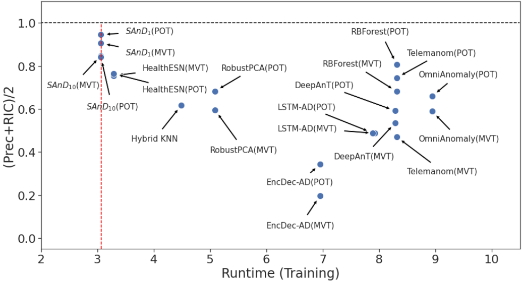
Figure 7: Performance for long-lived anomalies (y-axis) vs runtime (x-axis) concerning the training set, for both MVT and POT (Hybrid KNN uses the threshold $\Pr>0.8$). Runtimes are averages of the logarithm of seconds needed.

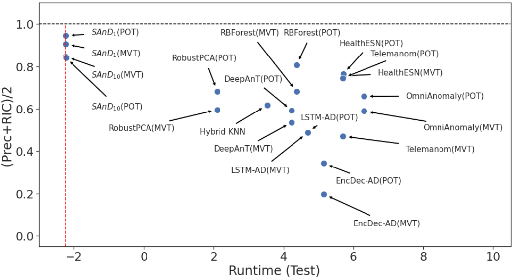
Figure 8: Performance for long-lived anomalies (y-axis) vs runtime (x-axis) concerning the test set, for both MVT and POT (Hybrid KNN uses the threshold $\Pr>0.8$). Runtimes are averages of the logarithm of seconds needed.

Appendix D KNN

Table 5 reports the performance metrics for Hybrid KNN when the threshold is set at 0.9 and 0.99. The results show that increasing probability does not increase performance. This is because Hybrid KNN gives a high probability to both true and false positives.

Method	MCC	F1	Prec	RIC	Rec	%No anomalies
Hybrid KNN
$\Pr>0.9$	0.169(0.28)	0.306(0.40)	0.320(0.18)	0.896(0.20)	0.708(0.20)	0.0%
$\Pr>0.99$	0.274(0.31)	0.336(0.43)	0.384(0.22)	0.855(0.22)	0.625(0.21)	0.0%

Table 5: Performance metrics of Hybrid KNN with probability threshold at 0.9 and 0.99.

Appendix E RIC

Assume that $J$ long-lived anomalies occur in $\mathbf{X}_{B}$. Let $TP_{j}$ be the number of true positives in the confusion matrix relative to long-lived anomaly $j$, $j=1\dots,J$. We consider the function $f(TP_{j})=1$ if $TP_{j}>0$ and $f(TP_{j})=0$ otherwise. Let a long-lived anomaly be indicated as a cluster, we define the ratio of identified clusters ($RIC$), as $RIC=\frac{\sum_{j}f(TP_{j})}{J}$.

Appendix F Focusing on long-lived anomalies

Here is an example of how we selected long-lived anomalies. Figure 9 shows the anomalies in the test set for the SMD 2-2 dataset (the second dataset that we considered from the SMD collection). Plot (a) shows the total anomalies, 2 short-lived and 3 long-lived. In our analysis, we focused on the anomalies shown in plot (b). This selection was repeated for all the 8 datasets considered. Figure 10 shows the anomalies in the test set for the SMD 1-1 dataset. Plot (a) shows the 8 anomalies, while plot (b) shows the 5 long-lived of interest in Section 5. Figure 11 reports in each plot the data used to obtain the results in Table 3.

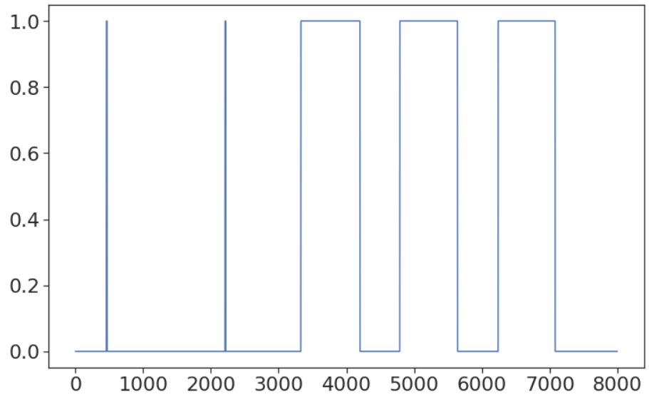
(a)

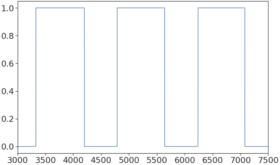
(b)

Figure 9: Anomalies on the test set of the SMD 2-2 dataset. Plot (a) reports all the anomalies. Plot (b) reports the long-lived ones.

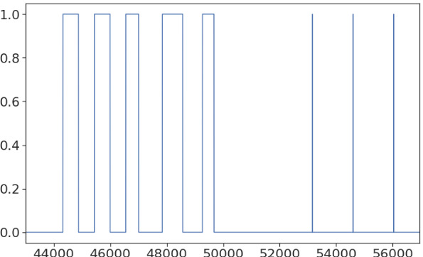
(a)

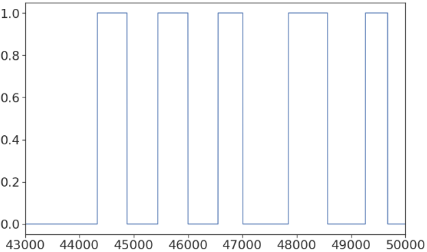
(b)

Figure 10: Anomalies on the test set of the SMD 1-1 dataset. Plot (a) reports all the anomalies. Plot (b) reports the long-lived ones.

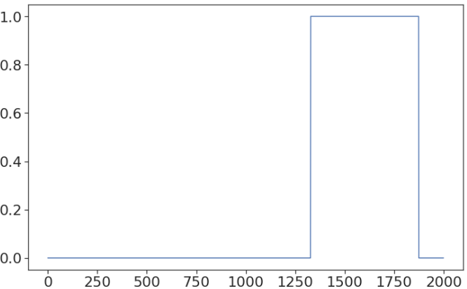
(a)

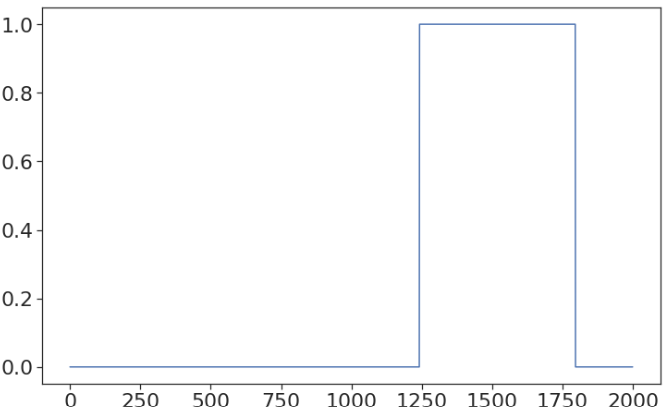
(b)

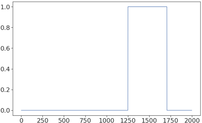
(c)

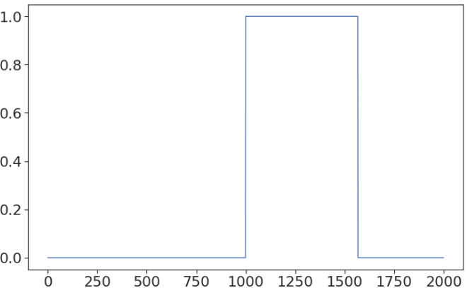
(d)

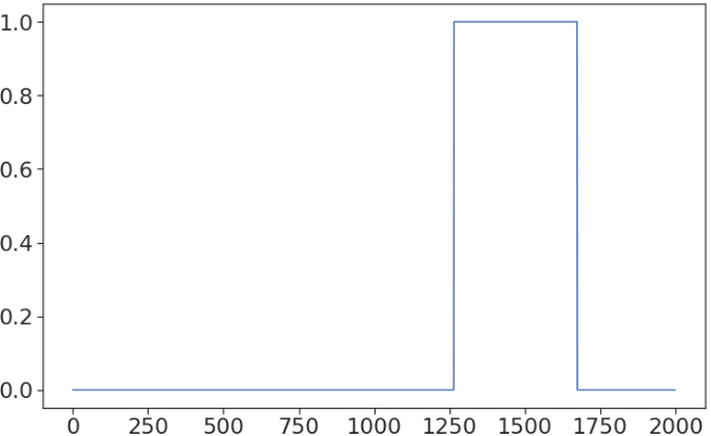
(e)

Figure 11: Panels (a)-(e) show the 5 datasets of size 2 000 (1 000 observations from the test set and 1 000 additional observations from the training set) concerning the long-lived anomlies of the 1-1 SMD dataset.

Appendix G Feature Importance

Figure 4 reports the ranking of the Gini index provided by the random forest in the case of $h=1$ (the higher is the value, the more important is the variable). It might be interesting to use this value to automatically decide how many variables $n$ to report to the user. For example, Figure 12 (a),(c),(d),(e) show that the variables 10, 12 and 13 are the most relevant for the corresponding anomalies. Similarly, Figure 13 reports the RCDE for $h=1$. Figures 14 and 15 report the Gini index and the RCDE rankings, respectively, in the case of $h=10$.

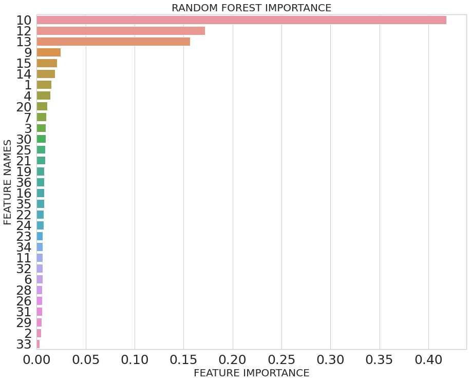
(a)

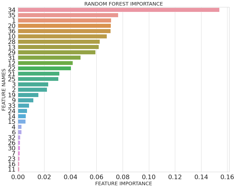
(b)

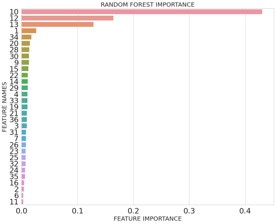
(c)

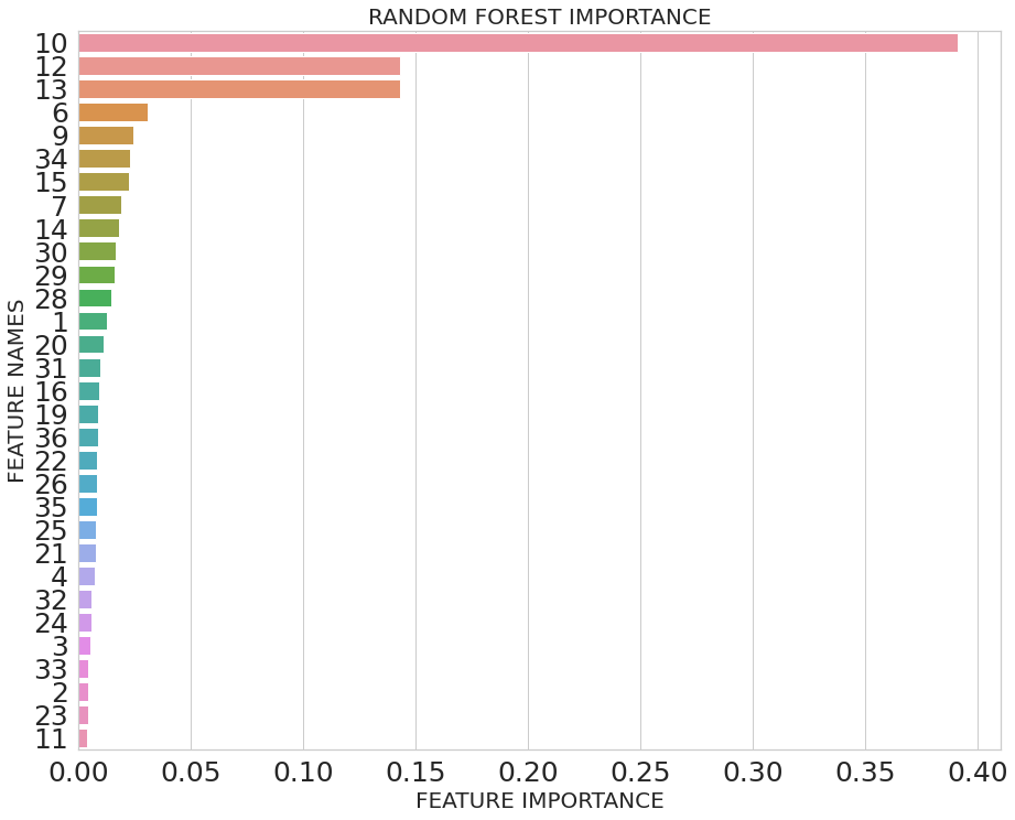
(d)

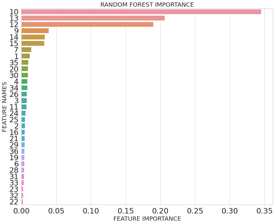
(e)

Figure 12: Variables importance as computed by our methodology for the 5 long-lived anomalies for $h=1$ (Anomaly 1 - Anomaly 5). The $x$-axis shows the value of the Gini index. The $y$-axis reports the label of the variables in increasing order of the Gini index.

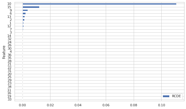
(a)

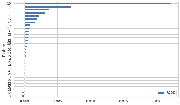
(b)

(c)

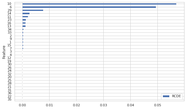
(d)

(e)

Figure 13: Variables importance as computed by our methodology for the 5 long-lived anomalies for $h=1$ (Anomaly 1 - Anomaly 5). The $x$-axis shows the value of the RCDE. The $y$-axis reports the label of the variables in increasing order of the RCDE.

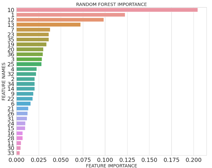
(a)

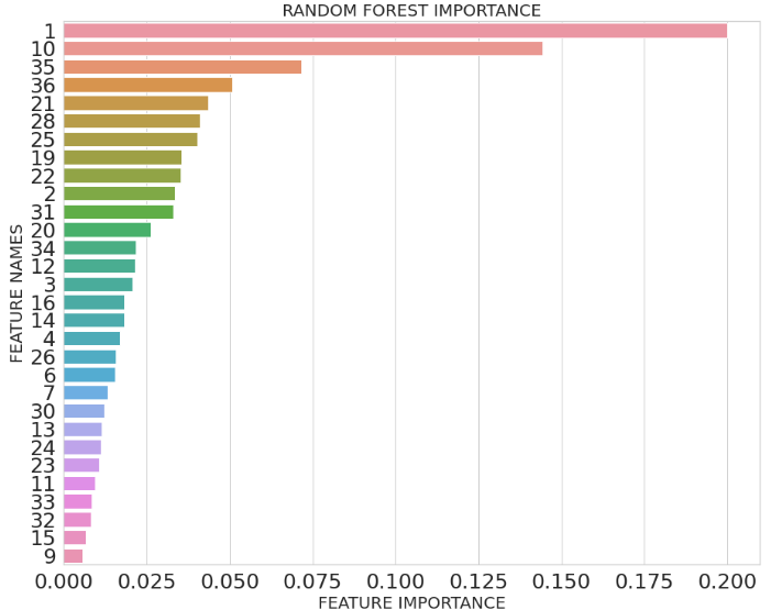
(b)

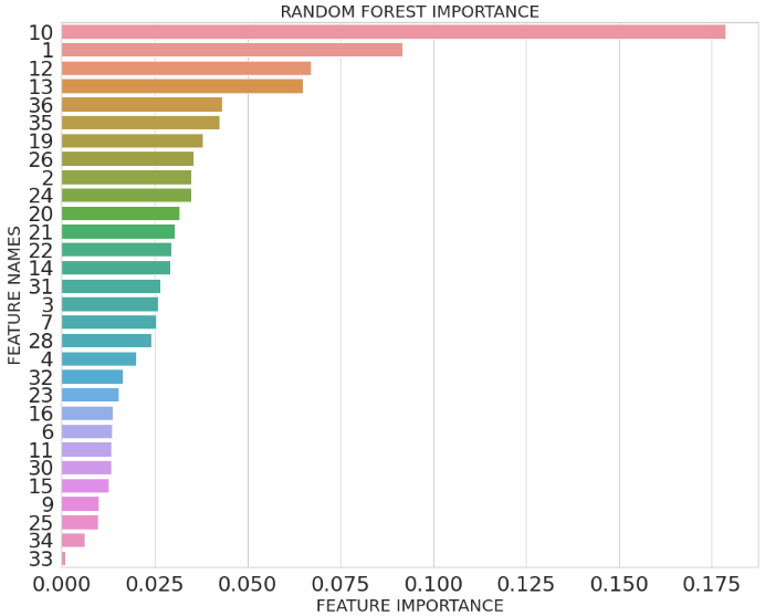
(c)

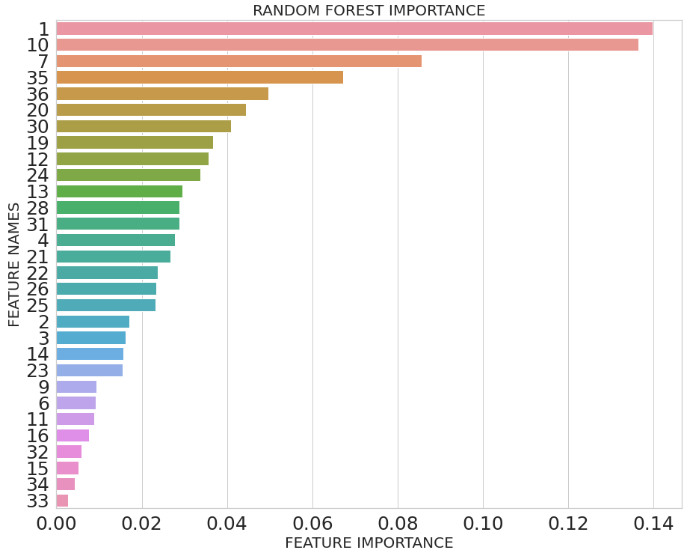
(d)

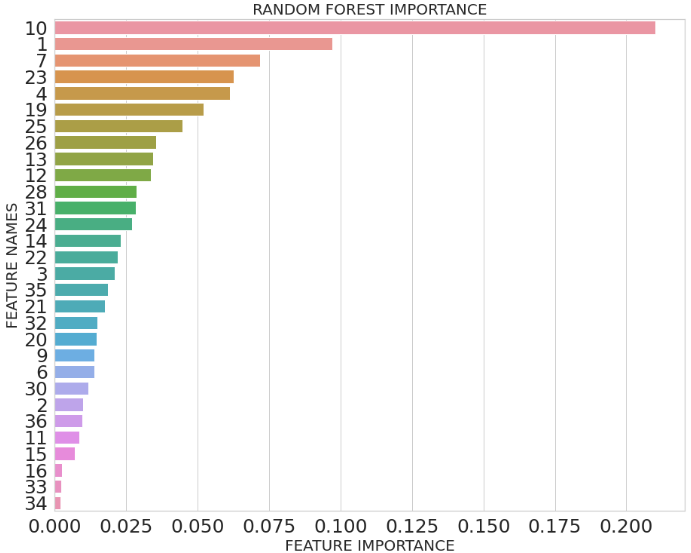
(e)

Figure 14: Variables importance as computed by our methodology for the 5 long-lived anomalies for $h=10$ (Anomaly 1 - Anomaly 5). The $x$-axis shows the value of the Gini index. The $y$-axis reports the label of the variables in increasing order of the Gini index.

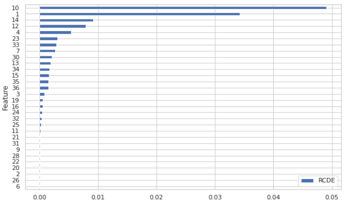
(a)

(b)

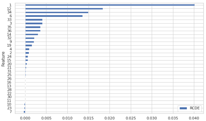
(c)

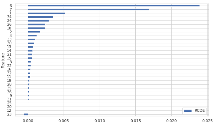
(d)

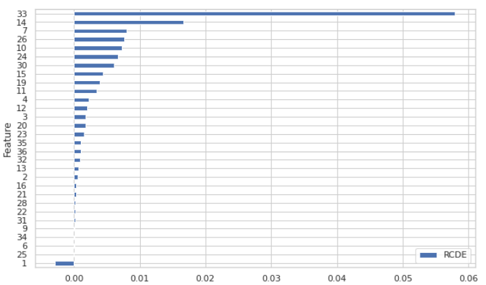
(e)

Figure 15: Variables importance as computed by our methodology for the 5 long-lived anomalies for $h=10$ (Anomaly 1 - Anomaly 5). The $x$-axis shows the value of the RCDE. The $y$-axis reports the label of the variables in increasing order of the RCDE.

Appendix H Analysis of the Short-Lived Anomaly for POT and $h=10$

Figure 16 reports the short-lived anomaly obtained by running ${\mathit{SAnD}}_{10}$ thresholded with POT. It lasts 20 seconds, so it is not due to sensor noises that last only one second. We run a random forest on the 100 observations reported in Figure 16, to maintain a ratio between the anomaly and the anomaly-free observations $\approx 0.25$, as in the case of the long-lived anomaly in Figure 5 (d). The 5 top variables are ReelPower, DR1PowerConsumption, ReelSpeed, MCC4PowerConsumption, and YankePressure. All these variables are still related to overheating of the system.

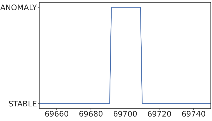
Figure 16: The short-lived anomaly detected by ${\mathit{SAnD}}_{10}$ and reported in Figure 16 (c).

References

- Alampalli (2000) Alampalli, S. (2000). Effects of testing, analysis, damage, and environment on modal parameters. Mechanical Systems and Signal Processing 14(1), 63–74.
- Balkema and De Haan (1974) Balkema, A. A. and L. De Haan (1974). Residual life time at great age. The Annals of probability 2(5), 792–804.
- Bart et al. (2001) Bart, P., M. Johan, and D. R. Guido (2001). Vibration-based damage detection in civil engineering. Smart materials and structure 10(3), 518.
- Bashar and Nayak (2020) Bashar, M. A. and R. Nayak (2020). Tanogan: Time series anomaly detection with generative adversarial networks. In 2020 IEEE SSCI, pp. 1778–1785. IEEE.
- Blázquez-García et al. (2021) Blázquez-García, A., A. Conde, U. Mori, and J. A. Lozano (2021). A review on outlier/anomaly detection in time series data. ACM Computing Surveys 54(3), 1–33.
- Breiman (2001) Breiman, L. (2001). Random forests. Machine Learning 45(1).
- Breiman et al. (1984) Breiman, L., J. Friedman, R. Olshen, and C. Stone (1984). Classification and Regression Trees. Monterey, CA: Wadsworth and Brooks.
- Cabana et al. (2019) Cabana, E., R. Lillo, and H. Laniado (2019). Multivariate outlier detection based on a robust mahalanobis distance with shrinkage estimators. Statistical Papers 62(4).
- Campos-Sánchez et al. (2016) Campos-Sánchez, R., M. A. Cremona, A. Pini, F. Chiaromonte, and K. D. Makova (2016). Integration and fixation preferences of human and mouse endogenous retroviruses uncovered with functional data analysis. PLoS computational biology 12(6), e1004956.
- Chen et al. (2020) Chen, Q., A. Zhang, T. Huang, Q. He, and Y. Song (2020). Imbalanced dataset-based echo state networks for anomaly detection. Neural Computing and Applications 32, 3685–3694.
- Chicco and Jurman (2020) Chicco, D. and G. Jurman (2020). The advantages of the matthews correlation coefficient (mcc) over f1 score and accuracy in binary classification evaluation. BMC genomics 21(1), 1–13.
- Choi et al. (2021) Choi, K., J. Yi, C. Park, and S. Yoon (2021). Deep learning for anomaly detection in time-series data: review, analysis, and guidelines. IEEE Access.
- Craney and Surles (2002) Craney, T. A. and J. G. Surles (2002). Model-dependent variance inflation factor cutoff values. Quality Engineering 14(3), 391–403.
- Deraemaeker and Worden (2018) Deraemaeker, A. and K. Worden (2018, 05). A comparison of linear approaches to filter out environmental effects in structural health monitoring. MSSP 105, 1–15.
- Filonov et al. (2016) Filonov, P., A. Lavrentyev, and A. Vorontsov (2016). Multivariate industrial time series with cyber-attack simulation: Fault detection using an lstm-based predictive data model.
- Fisher and Tippett (1928) Fisher, R. A. and L. H. C. Tippett (1928). Limiting forms of the frequency distribution of the largest or smallest member of a sample. In Mathematical proceedings of the Cambridge philosophical society, Volume 24, pp. 180–190. Cambridge University Press.
- Fithian and Hastie (2014) Fithian, W. and T. Hastie (2014). Local case-control sampling: Efficient subsampling in imbalanced data sets. Annals of statistics 42(5), 1693.
- Gnedenko (1943) Gnedenko, B. (1943). Sur la distribution limite du terme maximum d’une serie aleatoire. Annals of mathematics, 423–453.
- Grosskopf et al. (2022) Grosskopf, M., K. Myers, E. Lawrence, and D. Bingham (2022). Temporal characterization and filtering of sensor data to support anomaly detection. Technometrics 64(4), 475–486.
- Hubert and Van der Veeken (2008) Hubert, M. and S. Van der Veeken (2008). Outlier detection for skewed data. Journal of Chemometrics 22(3-4), 235–246.
- James et al. (2013) James, G., D. Witten, T. Hastie, and R. Tibshirani (2013). An introduction to statistical learning: with applications in R.
- Kyle et al. (2018) Kyle, H., C. Valentino, L. Christopher, C. Ian, and S. Tom (2018). Detecting spacecraft anomalies using lstms and nonparametric dynamic thresholding. In KDD, pp. 387–395.
- Mahalanobis (1936) Mahalanobis, P. C. (1936). On the generalized distance in statistics. NISI.
- Malhotra et al. (2016) Malhotra, P., A. Ramakrishnan, G. Anand, L. Vig, P. Agarwal, and G. Shroff (2016). Lstm-based encoder-decoder for multi-sensor anomaly detection. CoRR abs/1607.00148.
- Malhotra et al. (2015) Malhotra, P., L. Vig, G. Shroff, P. Agarwal, et al. (2015). Long short term memory networks for anomaly detection in time series. In Esann, Volume 2015, pp. 89.
- Maronna et al. (2019) Maronna, R. A., R. D. Martin, V. J. Yohai, and M. Salibián-Barrera (2019). Robust statistics: theory and methods (with R). John Wiley & Sons.
- Munir et al. (2018) Munir, M., S. A. Siddiqui, A. Dengel, and S. Ahmed (2018). Deepant: A deep learning approach for unsupervised anomaly detection in time series. Ieee Access 7, 1991–2005.
- Ogbechie et al. (2017) Ogbechie, A., J. Díaz-Rozo, P. Larrañaga, and C. Bielza (2017). Dynamic bayesian network-based anomaly detection for in-process visual inspection of laser surface heat treatment. In Machine Learning for Cyber Physical Systems, pp. 17–24. Springer.
- Paffenroth et al. (2018) Paffenroth, R., K. Kay, and L. Servi (2018). Robust PCA for anomaly detection in cyber networks. arXiv preprint arXiv:1801.01571.
- Peeters and De Roeck (2001) Peeters, B. and G. De Roeck (2001). One-year monitoring of the z24-bridge: environmental effects versus damage events. Earthquake engin. & structural dynamics 30(2), 149–171.
- Penny (1996) Penny, K. I. (1996). Appropriate critical values when testing for a single multivariate outlier by using the mahalanobis distance. Journal of the Royal Statistical Society: Series C (Applied Statistics) 45(1), 73–81.
- Pickands III (1975) Pickands III, J. (1975). Statistical inference using extreme order statistics. the Annals of Statistics, 119–131.
- Rousseeuw and Leroy (2005) Rousseeuw, P. J. and A. M. Leroy (2005). Robust regression and outlier detection. Wiley.
- Rousseeuw and van Zomeren (1990) Rousseeuw, P. J. and B. C. van Zomeren (1990). Unmasking multivariate outliers and leverage points. Journal of the American Statistical Association 85(411), 633–639.
- Schmidl et al. (2022) Schmidl, S., P. Wenig, and T. Papenbrock (2022, may). Anomaly detection in time series: A comprehensive evaluation. Proc. VLDB Endow. 15(9), 1779–1797.
- Siffer et al. (2017) Siffer, A., P.-A. Fouque, A. Termier, and C. Largouet (2017). Anomaly detection in streams with extreme value theory. In KDD’17, pp. 1067–1075. ACM.
- Song et al. (2017) Song, H., Z. Jiang, A. Men, B. Yang, et al. (2017). A hybrid semi-supervised anomaly detection model for high-dimensional data. Computational intelligence and neuroscience 2017.
- Su et al. (2019) Su, Y., Y. Zhao, C. Niu, R. Liu, W. Sun, and D. Pei (2019). Robust anomaly detection for multivariate time series through stochastic RNN. In KDD’19, pp. 2828–2837. ACM.
- Tiku et al. (2010) Tiku, M. L., M. Q. Islam, and S. B. Qumsiyeh (2010). Mahalanobis distance under non-normality. Statistics 44(3), 275–290.
- Todeschini et al. (2013) Todeschini, R., D. Ballabio, V. Consonni, F. Sahigara, and P. Filzmoser (2013). Locally centred mahalanobis distance. Analytica Chimica Acta 787, 1–9.
- Tripodi et al. (2020) Tripodi, G., F. Chiaromonte, and F. Lillo (2020). Knowledge and social relatedness shape research portfolio diversification. Scientific reports 10(1), 14232.