FedCRL: Personalized Federated Learning with Contrastive Shared Representations for Label Heterogeneity in Non-IID Data

Abstract

To deal with heterogeneity resulting from label distribution skew and data scarcity in distributed machine learning scenarios, this paper proposes a novel Personalized Federated Learning (PFL) algorithm, named Federated Contrastive Representation Learning (FedCRL). FedCRL introduces contrastive representation learning (CRL) on shared representations to facilitate knowledge acquisition of clients. Specifically, both local model parameters and averaged values of local representations are considered as shareable information to the server, both of which are then aggregated globally. CRL is applied between local representations and global representations to regularize personalized training by drawing similar representations closer and separating dissimilar ones, thereby enhancing local models with external knowledge and avoiding being harmed by label distribution skew. Additionally, FedCRL adopts local aggregation between each local model and the global model to tackle data scarcity. A loss-wise weighting mechanism is introduced to guide the local aggregation using each local model’s contrastive loss to coordinate the global model involvement in each client, thus helping clients with scarce data. Our simulations demonstrate FedCRL’s effectiveness in mitigating label heterogeneity by achieving accuracy improvements over existing methods on datasets with varying degrees of label heterogeneity.

I Introduction

I-A Background and Motivation

Empowered by Deep Learning (DL), data-driven learning approaches have gained popularity and demonstrated promise, while requiring substantial training datasets to achieve satisfactory results [1, 2]. However, in practice, training data is usually not available for centralization due to privacy concerns [3]. As a result, Federated Learning (FL), a distributed paradigm that allows clients to collaboratively train models without centralizing data, has emerged as a prevalent solution. The classical FL algorithm, FedAvg [4], performs well on Independent and Identically Distributed (IID) data. However, due to differences in geography and preferences among the devices and users, clients often have non-IID data, also called statistical heterogeneity [5], which poses challenges to traditional FL. This paper is motivated to mainly focus on two types of statistical heterogeneity as shown below.

• Label distribution skew: Label distribution skew refers to the FL situation where the distribution of labels varies significantly across different clients [6, 7, 8, 9]. For example, while one client’s data has a lot of samples of one class, another might have very few or none, leading to challenges in training a model that performs well across all clients due to these imbalances in label distribution.

• Data scarcity within data quantity skew: Data quantity skew among clients poses an additional challenge on fairness [7, 10], manifesting as data scarcity [11, 9]. On one hand, the labels of scarce data are sometimes unique and important, such as rare anomalies or surveys of minority groups. The difficulty of integrating the knowledge contained in scarce data into models of other clients leads to unfairness. On the other hand, scarce data is highly susceptible to causing overfitting, impeding normal local training. This usually occurs with monopolized clients or newly participating clients.

Consequently, the two types of statistical heterogeneity present significant challenges to FL, demanding prompt and effective solutions. Note that, since we mainly study the effect caused by labels in scarce data, data scarcity is also regarded as a kind of label skew in this paper. Thus, we collectively refer to the above two types of statistical heterogeneity as label heterogeneity. An illustration of the label heterogeneity is shown in Fig. 1.

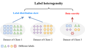
Figure 1: Illustration of label heterogeneity, where different shapes of graphics represent different labels.

To deal with label heterogeneity, Personalized Federated Learning (PFL) has emerged as an extension of traditional FL and received significant attention [5, 10]. PFL tailors personalized models for each client within a collaborative training paradigm to achieve robust performance on heterogeneous datasets. Notably, methods like FedProx [12], pFedMe [13], and Ditto [14] have been proven effective as they coordinate the distance between the global model and local models through regularizing the local training objective. Furthermore, a substantial body of research has focused on splitting the model structure into representation layers, serving as a common feature extractor, and projection layers which address specific tasks. Numerous algorithms have been proposed involving splitting the models communicated in FL and then designing hybrid learning strategies, such as FedPer [15], LG-FedAvg [16], MOON [17], FedRep [18]. Despite these advancements, the above methods only improve clients’ performance through generic model parameters but ignore more fine-grained characteristics inherent in data, especially label distribution skew. On the other hand, recent studies have explored data quantity skew problems [19, 11, 20, 21], but they have not adequately addressed co-existence of label distribution skew and data scarcity, leaving a research gap.

Thanks to the close correlation between data and representations [22], FedProto [23] pioneered the concept of utilizing representations as shareable information without privacy intrusion in FL, thus enhancing personalization through the provision of additional knowledge to clients. Building on this concept, recent studies, such as FedGH [24] and FedPAC [25], have integrated shared representations with the global model to balance the extraction of insights from both models and representations, achieving notable improvements. Nevertheless, a commonality among these methods is their focus on harnessing knowledge from representations with identical labels. More specifically, both FedProto and FedPAC employ regularization by calculating the distance between same-label representations. FedGH uses local representations to supervise the training of global projection layers, also concentrating on the alignment of same-label representations. The limitation in these methods is the lack of collaboration across various labels, which may restrict FL’s generalizability on clients with extreme label distribution skew, as shown in Fig. 1, hindering the participation of clients with scarce data. In light of this, Contrastive Representation Learning (CRL) which emphasizes deriving knowledge from label-agnostic representations [26, 27, 28], offers a promising perspective. We believe that utilizing shared representations among clients can further contribute to mitigating label heterogeneity.

I-B Main Work and Contributions of FedCRL

This paper introduces a novel PFL approach leveraging CRL [26, 29], aiming to address the label heterogeneity caused by label distribution skew and data scarcity in distributed ML scenarios. Leveraging shared representations, we orchestrate the aggregation of local models and local personalized training in a CRL-oriented perspective. During the FL communication, each client uploads local model parameters and the averaged local representations of each label to the server, and downloads globally aggregated model parameters and representations. Local representations are generated by feeding raw data into the representation layers. For example, if a client has data with two labels while totally five labels exist among all clients, this client needs to upload two averaged local representations and download five globally aggregated representations in each FL iteration. Both the architecture-agnostic model parameters and averaged representations will not intrude privacy.

During the local update, we sequentially conduct local aggregation and local training. To mitigate label distribution skew, CRL is adopted to regularize the local training, fostering similarity among representations with the same label and divergence among those with different labels. The global representations are used to construct positive and negative sample pairs for the local representations. Besides, to coordinate personalization among clients with significant data quantity skew, especially for data-scarce clients, a loss-wise weighting mechanism is introduced for local adaptive aggregation. This mechanism ensures that, when the local model’s contrastive loss is high, indicating its poor capability of distinguishing samples with different labels, the global model contributes more to drive advancement. Conversely, when the local model’s contrastive loss is low, the global model participates less to avoid a compromise on personalization. This mechanism is not affected by overfitting caused by data scarcity, because overfitting only occurs in supervised learning objectives, while contrastive loss is a form of self-supervised learning.

The contributions of this work are as follows:

• We introduce CRL into PFL to deal with label heterogeneity arising from label distribution skew and data scarcity, where averaged local representations of identical labels are regarded as shareable information between the clients and the server. By minimizing the distance between shared representations with identical labels and maximizing the distance between those with different labels, CRL can transfer additional knowledge of clients with abundant data to clients with scarce data without intruding data privacy.

• We propose Federated Contrastive Representation Learning (FedCRL) to guide personalization among clients with heterogeneous labels and data quantity skew. Specifically, FedCRL enhances each client’s knowledge through CRL on positive-negative sample pairs which are constructed by shared local representation and the global representations. Then local aggregation is conducted based on the contrastive loss. FedCRL is designed to address label heterogeneity, thus enhancing overall performance and fairness among clients.

• Theoretical analysis for the effectiveness of the designed local loss function and the communication convergence of the proposed FL algorithm is provided. Moreover, in the experiments on image datasets with varying degrees of data heterogeneity, we demonstrate the superiority of FedCRL compared to existing methods, showing the best averaged performance of local models. Besides, we also demonstrate FedCRL’s improved scalability and fairness on clients with scarce data.

The remainder of this paper is organized as follows. Section II reviews the related work of FL and CRL. Section III presents the formulation of PFL, representation sharing, and the developed FedCRL algorithm. Section IV analyzes the effectiveness of the designed loss function and the non-convex convergence of the developed algorithm. The experimental results and discussions are provided in Section V. Section VI concludes the whole paper.

II Literature Review

II-A FL Methods

Traditional FL methods like FedAvg [4], which learn a single global model for all clients, excel with IID data but suffer on non-IID data. FedProx [12] and Ditto [14] mitigate the impact of heterogeneity by regulating the L2 distance between local models and the global model, while pFedMe [13] learns an additional model for each client. To deal with device heterogeneity, PerFedAvg integrates meta learning with FL [30]. However, these methods become less effective with diverse data or numerous clients.

Model splitting has gained traction in FL, and representative works include FedPer [15], LG-FedAvg [16], and FedRep [18], which split model layers for global aggregation. Besides, exploration into client-tailored aggregations, like FedAMP [31] and FedALA [32], aligns with our method. While effective in managing data heterogeneity, these methods only conduct personalization based on model parameters instead of features inherent in raw data. Notably, in MOON [17], CRL is applied to clients, but only between the local model and global model, neglecting the interactions between clients.

On the other hand, data quantity skew has been studied by combining few-shot learning and FL. Federated Few-Shot Learning (FedFSL) emerges as a pivotal approach to address few-shot tasks in distributed settings. Initiated by the work [19], it leverages mutual information and a two-stage adversarial learning for consistent feature space development across local and global models, showcasing effectiveness in data-scarce environments. The work of [21] further defines FedFSL, focusing on optimizing new task performance with limited samples through meta task formulation. Meanwhile, the works of [11] explores model-agnostic FL to bridge domain gaps and enhance data-scarce clients’ knowledge. The work of [20] integrates relation network into FL to develop a lightweight framework for distributed few-shot image classification. Since scenarios with both label distribution skew and data scarcity have not been considered sufficiently, a research gap is remained.

Drawing from representation learning [22], FedProto [23] proposes to share local representations between clients and server and use them for regularization, while FedGH [24] uploads local representations to train a global projection layer. FedPAC [25] leverages representations to optimize local classifier combination for a balance between bias and variance. While the above models achieve good performance on heterogeneous data, there remains untapped potential in utilizing shared representations for enhancement. In contrast, our work achieves information enhancement and local aggregation for all clients through CRL on shared representations.

II-B Contrastive Representation Learning

CRL, an emergent field in self-supervised learning, excels in capturing knowledge from unlabeled data [26, 27, 33]. Its effectiveness hinges on the principle of minimizing the distance between representations with identical labels (positive pairs) and maximizing that between representations with different labels (negative pairs). Though there exist works of integrating CRL with FL [33, 17], CRL among shared representations, we believe as a significant perspective, has not been explored. Due to the self-supervised nature [34], CRL can deal with data scarcity in FL by extracting features from small-dataset clients. Since the distinctiveness of data has yet not been adequately considered in FL communications, CRL is promising to bridge this gap by guiding models to learn distinctive and fine-grained features from small datasets, while maintaining coherence with the global model. Thus, we propose FedCRL by learning knowledge from both model parameters and representations in this work.

III Methodology

III-A Problem Statement

We consider $N$ clients, and for the $i$th client, a local model $\theta^{i}$ is deployed to conduct training on a dataset $\mathcal{D}^{i}$. For each sample-label pair $(\mathbf{x}^{i},\mathbf{y}^{i})\sim\mathcal{D}^{i}$, the local model $f_{\theta^{i}}$, where $\theta^{i}:\mathbb{R}^{d}\to\mathcal{Y}$ is the parameter set, maps $\mathbf{x}^{i}\in\mathbb{R}^{d}$ to predict $\hat{\mathbf{y}}^{i}=f_{\theta^{i}}(\mathbf{x}^{i})\in\mathbb{Y}$ to resemble the true label $\mathbf{y}^{i}$. All clients have the same objective to improve the performance, in specific, to minimize the empirical risk over local datasets:

$$\mathcal{F}:=\mathbb{E}_{(\mathbf{x}^{i},\mathbf{y}^{i})\sim\mathcal{D}^{i}}\mathcal{L}(\mathbf{x}^{i},\mathbf{y}^{i};\theta^{i}),$$ (1)

where $\mathcal{L}:\mathcal{Y}\times\mathcal{Y}\to\mathbb{R}$ is the loss function of the specific ML task to penalize the distance between $\mathbf{y}^{i}$ and $\hat{\mathbf{y}}^{i}$. The primary goal of the server is to personalize $\{\theta^{i}\}_{i=1}^{N}$ for each client to minimize $\mathcal{F}$. Thus, the global objective is to find a set of local model parameters $\Theta^{*}=\{\theta^{i*}\}_{i=1}^{N}$ which satisfy

$$\Theta^{*}=\arg\min_{\Theta^{*}}\frac{1}{N}\sum_{i=1}^{N}\mathcal{F}^{i},$$ (2)

where $\mathcal{F}^{i}:=\mathcal{F}(\theta^{i*},\mathcal{D}^{i})$ is the personalized objective of the $i$th client.

III-B Representations Shared in FL

Heterogeneous data distributed across tasks may share a common representation despite having different labels [22]. Inspired by insights from [18, 23] that representations shared among clients, e.g., shared features across many types of images or across word-prediction tasks, may provide auxiliary information without privacy intrusion, we consider utilizing shared representations to assist local adaptive aggregation and local personalized training.

Briefly, we let $f_{\theta^{i}}=[f_{\phi^{i}};f_{\pi^{i}}]$, where $f_{\phi^{i}}(\cdot)$ is the representation layers of the $i$th local model used to generate representations, and $f_{\pi^{i}}(\cdot)$ is the projection layers for the output. For the $i$th client, a local representation $\bar{\omega}^{i}_{c}\in\mathbb{R}^{k}$ is the mean value of the representations of the label $c\in\mathcal{C}^{i}$, where $\mathcal{C}^{i}$ contains all labels in $\mathcal{D}^{i}$. Then, we denote $\mathcal{D}^{i}_{c}$ as the subset of $\mathcal{D}^{i}$ only containing samples of label $c$, and $\omega^{i}=f_{\phi^{i}}(\mathbf{x}^{i})\in\mathbb{R}^{k}$ as the representation of $\mathbf{x}^{i}$. Formally, the representation of type $c$ can be calculated as:

$$\bar{\omega}^{i}_{c} =\frac{1}{|\mathcal{D}^{i}_{c}|}\sum_{\mathbf{x}^{i}\in\mathcal{D}^{i}_{c}}\omega^{i},\quad c\in\mathcal{C}^{i}.$$ (3)

Also, we denote $f_{\phi^{i}}(\cdot)\in\mathbb{R}^{d\times k}$ and $f_{\pi^{i}}(\cdot)\in\mathbb{R}^{k}$ as mapping matrices. Note that $k\ll d$, which is widely applied to reduce the communication overhead. By collecting representations of all labels in $\mathcal{D}^{i}$, the local representations of the $i$th client can be denoted as:

$$\bar{\Omega}^{i} =\{\bar{\omega}^{i}_{c}|c\in\mathcal{C}^{i}\}.$$ (4)

To obtain the final prediction, $f_{\pi^{i}}(\cdot)$ maps $\omega^{i}$ to the label space. In other words, $f_{\theta^{i}}(\mathbf{x}^{i})$ equals to $f_{\pi^{i}}(\omega^{i})$.

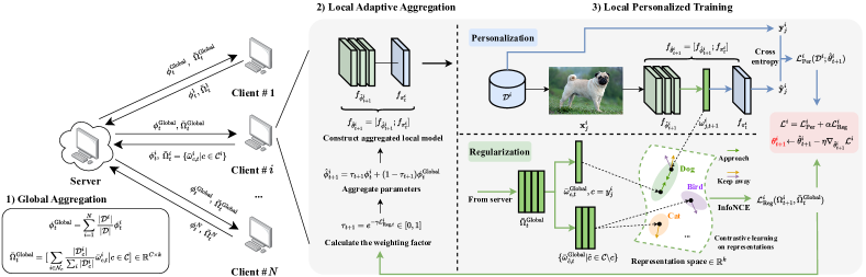
Figure 2: The entire process of FedCRL.

III-C Our Developed FedCRL

At each iteration, the server conducts global aggregation on local models and local representations to generate the global parameters and global representations. Then all clients download the global information for local updates. The main processes of the local update include two parts: local adaptive aggregation by loss-wise weighting and local personalized training by CRL. The overall architecture of FedCRL is shown in Fig. 2.

III-C1 Global Aggregation

Shallow layers can learn more generic information and they are more suitable for sharing [35, 1]. In FedCRL, clients only send the parameters of representation layers $\phi$ to the server for aggregation and keep the parameters of projection layers $\pi$ local for maintaining the personalization. Also, it is robust for privacy preservation to drop the last one or multiple layers to avoid reverse engineering [36]. Thus, different from the traditional global model aggregation [4], the server in FedCRL aggregates $\{\phi^{i}_{t}\}^{N}_{i=1}$ at iteration $t$ as follows:

$$\phi^{\text{Global}}_{t}=\sum_{i=1}^{N}\frac{|\mathcal{D}^{i}|}{|\mathcal{D}|}\phi^{i}_{t},$$ (5)

where $\mathcal{D}=\{\mathcal{D}^{i}\}_{i=1}^{N}$ contains all clients’ datasets. Beside the parameter aggregation, all clients upload local representations to the server for aggregation as:

$$\bar{\Omega}^{\text{Global}}_{t}=\big{[}\sum_{i\in\mathcal{N}_{c}}\frac{|\mathcal{D}^{i}_{c}|}{\sum_{i}|\mathcal{D}^{i}_{c}|}\bar{\omega}^{i}_{c,t}\big{|}c\in\mathcal{C}\big{]}\in\mathbb{R}^{C\times k},$$ (6)

where $\mathcal{N}_{c}$ denotes the set of clients owning samples of label $c$, and $\mathcal{C}=\bigcup_{i=1}^{N}\mathcal{C}^{i}$ is the total labels existing in all clients. Rather than averaging, the label volume-wise weighting is adopted for the global representation aggregation by considering the size of $\mathcal{D}^{i}_{c}$, mitigating the compromise on the global representations caused by inefficient local representations of the labels with scarce samples.

III-C2 Local Adaptive Aggregation

When completing the global aggregation at iteration $t$, we start the local update at iteration $t+1$, which begins with the initial step of local adaptive aggregation. This mechanism guides local models to aggregate a proportion of global model parameters corresponded to their own model performance, in order to achieve adaptive personalization. Different from traditional FL overwriting local models by the global model, the $i$th client aggregates $\phi^{i}_{t}$ with $\phi^{\text{Global}}_{t}$. In advance, we introduce the contrastive loss $\mathcal{L}^{i}_{\text{Reg},t}$ at iteration $t$, which will be elaborated in Section III-C3. To conduct local adaptive aggregation, a weighting factor $\tau_{t+1}$ is determined by exponentially scaling $\mathcal{L}^{i}_{\text{Reg},t}$ into $[0,1]$. Then, the $i$th client conducts local aggregation and obtains the aggregated local model $f_{\hat{\theta^{i}}_{t+1}}$ for further local training, formulated as follows:

$$\tau_{t+1} =e^{-\gamma\mathcal{L}^{i}_{\text{Reg},t}}\in[0,1],\gamma>0,$$ (7)

$$\hat{\phi}^{i}_{t+1} =\tau_{t+1}\phi^{i}_{t}+(1-\tau_{t+1})\phi_{t}^{\text{Global}},$$ (8)

$$f_{\hat{\theta}^{i}_{t+1}} =[f_{\hat{\phi}^{i}_{t+1}};f_{\pi^{i}_{t}}],$$ (9)

where $\gamma$ is a hyperparameter to control the sensitivity of scaling. When $\mathcal{L}^{i}_{\text{Reg},t}$ is higher, $\tau_{t+1}$ becomes smaller to draw on more parameters from the global model for knowledge enhancement. On the other hand, when $\mathcal{L}^{i}_{\text{Reg},t}$ is lower, the local model becomes less dependent on acquiring knowledge from the global model. The exponential design provides a type of nonlinear mapping, guiding the $i$th client to deal with iterations with high loss by learning from the global model.

The reason for choosing the contrastive loss as the basis for weighting, rather than the supervised loss, is that the contrastive loss directly reflects the model’s ability to distinguish among multiple samples with different labels. On the other hand, although the supervised loss can reflect the model’s recognition capability for individual samples, it tends to result in severe overfitting in clients with scarce data, leading to low training loss but poor predictive performance. Therefore, using the contrastive loss can objectively reflect the capability of each local model without being affected by data scarcity.

III-C3 Local Personalized Training

The data distributions are significantly different among clients due to heterogeneity. So it is necessary to consider both personalization for adapting patterns of local datasets and regularization for properly acquiring external information.

Personalization: For the $i$th client, we use $\mathcal{L}$ in Eq. (​​ 1) as the personalization objective $\mathcal{L}^{i}_{\text{Per}}$ based on the local dataset. In the context of classification task, we firstly randomly divide $\mathcal{D}^{i}$ into batches $\mathcal{D}^{i}_{b,t+1}$ for training efficiency, each of which has $b$ samples. Then we use the expectation of cross entropy to denote this objective at iteration $t+1$:

$$\mathcal{L}^{i}_{\text{Per},t+1}=\mathbb{E}_{\mathcal{D}^{i}_{b,t+1}\sim\mathcal{D}^{i}}\mathbb{E}_{(\mathbf{x}^{i}_{j},\mathbf{y}^{i}_{j})\sim\mathcal{D}^{i}_{b,t+1}}\big{[}H(\mathbf{y}^{i}_{j},\hat{\mathbf{y}}^{i}_{j})\big{]},$$

$$H(\mathbf{y}^{i}_{j},\hat{\mathbf{y}}^{i}_{j})=-\sum_{c=1}^{C}y^{i}_{j,c}\log(\hat{y}^{i}_{j,c}),$$ (10)

$$\mathbf{y}^{i}_{j}=f_{\hat{\theta}^{i}_{t+1}}(\mathbf{x}^{i}_{j})=(y^{i}_{j,1},...,y^{i}_{j,C}),\hat{\mathbf{y}}^{i}_{j}=(\hat{y}^{i}_{j,1},...,\hat{y}^{i}_{j,C}).$$

Through personalization, each client cares about local patterns and can adjust the distance between $\theta^{i}$ and $\theta^{\text{Global}}$.

Regularization: To utilize useful external information while maintaining the local personalization, we adopt CRL on representations for regularization.

Inspired by [26, 27], CRL, an ML technique aiming to learn representations by contrasting positive pairs (similar samples) against negative pairs (dissimilar samples), can be utilized between the local representations and the global representations to assist personalization. Specifically, at iteration $t+1$, the $i$th client receives the global representations $\bar{\Omega}^{\text{Global}}_{t}$ from the server. We assume that the labels unseen to $\mathcal{D}^{i}$ can provide external knowledge for $f_{\theta^{i}}$. We let $b$ be the batch size, and have representations $\Omega^{i}_{t+1}=\{\omega^{i}_{j,t+1}\}_{j=1}^{b}$ at iteration $t+1$ by forwarding $\{\mathbf{x}^{i}_{j}\}_{j=1}^{b}$ towards $f_{\hat{\phi}^{i}_{t+1}}$. Then, we construct positive pair and negative pairs for the $\omega^{i}_{j,t+1}$ by $\bar{\omega}^{\text{Global}}_{c,t}$ and {$\bar{\omega}^{\text{Global}}_{\hat{c},t}|\hat{c}\in\mathcal{C}\backslash c\}$, respectively, where the label of $\omega^{i}_{j,t+1}$ is $c$.

Definition 1 (Positive and Negative Pairs of Representations).

Intuitively, for $\omega^{i}_{j,t+1}$ whose label is $c$, we consider the same label in the global representation $\bar{\omega}^{\text{Global}}_{c,t}$ as the positive sample, while the remaining different labels are considered as negative samples. Since the global representations correspond one-to-one with all $|\mathcal{C}|$ label categories among all clients, one positive pair $p^{+}_{j,t+1}$ and $|\mathcal{C}|-1$ negative pairs $\{p^{-}_{j,t+1}\}$ are constructed as:

$$p^{+}_{j,t+1} =(\omega^{i}_{j,t+1},\bar{\omega}^{\text{Global}}_{c,t}),$$ (11)

$$\{p^{-}_{j,t+1}\} =\{(\omega^{i}_{j,t+1},\bar{\omega}^{\text{Global}}_{\hat{c},t})|\hat{c}\sim\mathcal{C}\backslash c\},$$

$$y^{i}_{j}=c, \quad i\in\{1,...,N\},\quad j\in\{1,...,b\}.$$

We adopt InfoNCE [26] as the form of regularization loss function, aiming to maximize the similarity of positive pairs and minimize the similarity of negative pairs. For the $i$th client, according to Definition. 1, the regularization loss can be expressed as:

$$\mathcal{L}^{i}_{\text{Reg},t+1}:=\mathbb{E}_{\mathcal{D}^{i}_{b,t+1}\sim\mathcal{D}^{i}}\mathbb{E}_{(\mathbf{x}^{i}_{j},\mathbf{y}^{i}_{j})\sim\mathcal{D}^{i}_{b,t+1}}$$ (12)

$$\Bigg{[}-\log\frac{e^{\big{[}D(p^{+}_{j,t+1})/\tau_{\text{CL}}\big{]}}}{e^{\big{[}D(p^{+}_{j,t+1})/\tau_{\text{CL}}\big{]}}+\sum_{\hat{c}\in\mathcal{C}\backslash c}e^{\big{[}D(p^{-}_{j,t+1})/\tau_{\text{CL}}\big{]}}}\Bigg{]},$$

$$D(\omega^{i}_{j,t+1},\bar{\omega}^{\text{Global}}_{c,t})=\frac{\omega^{i}_{j,t+1}\cdot\bar{\omega}^{\text{Global}}_{c,t}}{||\omega^{i}_{j,t+1}||_{2}\cdot||\bar{\omega}^{\text{Global}}_{c,t}||_{2}}\in[-1,1],$$

where $\tau_{\text{CL}}$ is the temperature of CRL which adjusts the attention on positive samples or negative samples, and $D(\cdot)$ is cosine similarity. Then, the $i$th client calculates the local representations $\bar{\Omega}^{i}_{t+1}$ by averaging $\Omega^{i}_{t+1}$ referring to Eq. (​​ 7) for the global aggregation.

Note that, the batch size $b$ in Eq. (​​ 12) not only affects training effect but also impacts the computational overhead, because a larger $b$ means more negative instances are utilized. For contrastive learning, more negative instances can bring about more knowledge enhancement, thereby improving the training effect but increasing the computational overhead, which needs to be carefully balaneced.

Final Objective:

As a result, we obtain the final objective function for locally updating $\theta^{i}$ at iteration $t$:

$$\mathcal{L}^{i}_{t+1}:=\mathcal{L}^{i}_{\text{Per},t+1}(\mathcal{D}^{i};\hat{\theta}^{i}_{t+1})+\alpha\mathcal{L}^{i}_{\text{Reg},t+1}(\Omega^{i}_{t+1},\bar{\Omega}^{\text{Global}}_{t}).$$ (13)

The process of local updates can be expressed as follows:

$$\theta^{i}_{t+1}\leftarrow\hat{\theta}^{i}_{t+1}-\eta\nabla_{\hat{\theta}^{i}_{t+1}}\mathcal{L}^{i}_{t+1}(\mathcal{D}^{i};\hat{\theta}^{i}_{t+1};\Omega^{i}_{t+1},\bar{\Omega}^{\text{Global}}_{t}),$$ (14)

where $\alpha$ is the hyperparameter for trading off personalization and regularization, and $\eta$ is the learning rate.

Algorithm 1 Training process of FedCRL

1:  Input: The server and $N$ clients; $\{\mathcal{D}^{i}\}_{i=1}^{N}$: datasets of $N$ clients; $\theta^{\text{Global}}_{0}$: the initial global model; $\eta$: the learning rate; $\alpha$: the trade-off factor between personalization and regularization.

2:  Output: $\theta^{1*},...,\theta^{N*}$: Optimal local model parameters.

3:  Initialization:

4:  The server sends $\theta^{\text{Global}}_{0}$ to all clients to initialize $\{\hat{\theta}^{i}_{0}\}_{i=1}^{N}$ by overwriting, rather than local aggregation in Eq. (​​ 8).

5:  Clients train $\{\hat{\theta}^{i}_{0}\}_{i=1}^{N}$ by Eq. (​​ 14) in parallel, where $\alpha=0$. Then clients get $\{\theta^{i}_{1}\}_{i=1}^{N}$.

6:  Clients collect $\{\bar{\Omega}^{i}_{1}\}_{i=1}^{N}$ by Eq. (​​ 3) and Eq. (​​ 4).

7:  Clients upload $\{\phi^{i}_{1}\}_{i=1}^{N}$ and $\{\bar{\Omega}^{i}_{1}\}_{i=1}^{N}$ to the server.

8:  FL Communication:

9:  for iteration $t=1,...,T$ do

10:       Server: $\blacktriangleright$ Global aggregation

11:       The server aggregates $\{\phi^{i}_{t}\}_{i=1}^{N}$ to get $\phi^{\text{Global}}_{t}$ by Eq. (​​ 5).

12:       The server aggregates $\{\bar{\Omega}^{i}_{t}\}_{i=1}^{N}$ to get $\bar{\Omega}^{\text{Global}}_{t}$ by Eq. (​​ 6).

13:       The server sends $\phi^{\text{Global}}_{t}$ and $\bar{\Omega}^{\text{Global}}_{t}$ to all clients.

14:       Clients:

15:       for the $i$th client in parallel do $\blacktriangleright$ Local Update

16:           Local Aggregation:

17:           Calculate $\tau_{t+1}$ based on $\mathcal{L}^{i}_{\text{Reg},t}$ by Eq. (​​ 7).

18:           Obtain local aggregated model $f_{\hat{\theta}^{i}_{t+1}}$ by Eq. (​​ 9).

19:           Local Training:

20:           Construct positive pairs and negative pairs by Eq. (​​ 11).

21:           Calculate $\mathcal{L}^{i}_{t+1}$ by Eq. (​​ 13).

22:           Train $\hat{\theta}^{i}_{t+1}$ by Eq. (​​ 14) and clip it into $[0,1]$ for normalization to get $f_{\theta^{i}_{t+1}}=[f_{\phi^{i}_{t+1}};f_{\pi^{i}_{t+1}}]$.

23:           Upload:

24:           Collect $\bar{\Omega}^{i}_{t+1}$ by Eq. (​​ 3) and Eq. (​​ 4).

25:           Upload $\phi^{i}_{t+1}$ and $\bar{\Omega}^{i}_{t+1}$ to the server.

26:       end for

27:  end for

28:  return $\theta^{1*},...,\theta^{N*}$.

Algorithm 1 presents the entire training process of FedCRL, including 1) global aggregation for both model parameters and representations (line 11-13); 2) local aggregation between each model and the global model (line 17-18); and 3) local training on the aggregated local model (line 20-22).

IV Theoretical Analysis

Before conducting experiments, we provide a theoretical analysis of the developed FedCRL algorithm. Firstly, we focus on the effectiveness of the local loss function incorporating cross entropy and InfoNCE, as the local training is the core part of the personalization of FedCRL. We explain that minimizing InfoNCE in FedCRL aims to maximize the mutual information between the local representations and global representations, thus enhancing the knowledge of each local model. Secondly, both global model aggregation and local model aggregation linearly change the model parameters, which may cause deviations in the loss expectation during each iteration. If the deviation is unbounded, the convergence of FedCRL may not be guaranteed. Therefore, we characterize the overall communication between the server and the clients to establish an upper bound on the loss expectation deviation, thereby ensuring the convergence of FedCRL. Note that due to the non-convexity of the local loss induced by InfoNCE, we focus on non-convex settings. Morevoer, we also present the relationship between the convergence rate and key hyperparameters.

IV-A Effectiveness of Local Loss Function

Referring to Eq. (13), the local loss function is a linear combination of $\mathcal{L}_{\text{Per}}$ and $\mathcal{L}_{\text{Reg}}$. Since $\mathcal{L}_{\text{Per}}$ is in the form of cross entropy, its convexity and good convergence are known [37]. But the non-convexity of InfoNCE $\mathcal{L}_{\text{Reg}}$ may lead to sub-optimum of the training objective for each local model. Thus, we focus on analyzing $\mathcal{L}_{\text{Reg}}$ to explain the effectiveness of the local loss function. Before presetting the analysis, we make the following assumption specifying that there are no outliers in $\mathcal{D}^{i}$, or the outliers have been removed, which is reasonable.

Assumption 1 (Sub-Gaussian Design).

Let $\forall\mathbf{x}^{i}\in\mathbb{R}^{d}$ be IID with mean $\mathbf{0}\in\mathbb{R}^{d}$ and covariance $\mathbf{I}_{d}\in\mathbb{R}^{d\times d}$. Thus, $\forall\mathbf{x}^{i}\in\mathbb{R}^{d}$ is $\mathbf{I}_{d}$-sub-Gaussian, i.e., $\mathbb{E}[e^{\mathbf{v}^{\top}\mathbf{x}^{i}}]\leq e^{\frac{||\mathbf{v}||_{2}^{2}}{2}},\forall\mathbf{v}\in\mathbb{R}^{d}$.

To quantify the enhancement brought by the InfoNCE loss $\mathcal{L}_{\text{Reg}}$, we introduce the manifestation of mutual information in contrastive learning as follows.

Definition 2 (Mutual Information in Contrastive Learning).

To construct contrastive learning task, mutual information is introduced between anchor samples $X$ and the similar samples $X^{+}$, also called positive sample:

$$I(X^{+};X)=\sum_{x^{+}\in X^{+},x\in X}p(x^{+},x)\log\bigg{[}\frac{p(x^{+}|x)}{p(x^{+})}\bigg{]}.$$ (15)

Based on Assumption 1 and Definition 2, we present the following theorem to illustrate the effectiveness of the local loss function design.

Theorem 1 (InfoNCE Minimization in FedCRL).

For each data batch of the $i$th client, minimizing InfoNCE equals to maximizing the mutual information between each anchor representation in this batch and its positive representation, and meanwhile minimizing the mutual information between it and its negative representations, formulated as follows, where $b$ is the batch size:

$$\mathcal{L}^{i}_{\text{Reg},t+1}\geq-\frac{1}{b}\sum_{j=1}^{b}I(\bar{\omega}^{\text{Global}}_{c,t},\omega^{i}_{j})+\log(C).$$ (16)

Intuitively, we have $\bar{I}(\cdot)\geq\log(C)-\mathcal{L}_{\text{Reg}}$, where $\bar{I}(\cdot)$ is the mean value of the mutual information. When $C$ becomes larger, the lower bound of similar representations increases, improving the performance of the $i$th local model. Theorem 1 indicates that optimizing the regularization term $\mathcal{L}^{i}_{\text{Reg}}$ can enlarge the information acquisition for the $i$th client, showing the effectiveness of combining $\mathcal{L}_{\text{Per}}$ and $\mathcal{L}_{\text{Reg}}$. Due to the page limitation, the proof of Theorem 1 is omitted from the current paper.

IV-B Convergence of FedCRL

The convergence conditions for the $i$th client is explained in this part. For ease of discussion, we denote the total number of local training epochs as $R$, which is set to 1 in this paper. Specifically, we define $tR+r$ as the $r$th epoch at iteration $t$, $tR$ as the end of iteration $t$ (end of the local training), $tR+0$ as the beginning of iteration $t$ (local aggregation), and $tR+\frac{1}{2}$ as the utilization of global representations at iteration $t$ (after local aggregation).

Before showing the convergence of FL communication, we make three assumptions which are widely used in literature: Assumption 2: Lipschitz Smoothness ensuring consistency in gradient changes [30, 12, 31, 23], Assumption 3: Unbiased Gradient and Bounded Variance providing stable gradient estimates [30, 12, 23], and Assumption 4: Bounded Variance of Representation Layers guaranteeing an acceptable variance between the global model and each local model.

Assumption 2 (Lipschitz Smoothness).

The $i$th local loss function is $L_{1}$-Lipschitz smooth, leading to that the gradient of the local loss function is $L_{1}$-Lipschitz continuous, where $L_{1}>0$, $\forall r_{1},r_{2}\in\{0,\frac{1}{2},1,...,R\}$, and $(\mathbf{x}^{i},\mathbf{y}^{i})\in\mathcal{D}^{i}$:

$$||\nabla\mathcal{L}^{i}_{tR+r_{1}}(\mathbf{x}^{i},\mathbf{y}^{i};\hat{\theta}^{i}_{tR+r_{2}})-\nabla\mathcal{L}^{i}_{tR+r_{2}}(\mathbf{x}^{i},\mathbf{y}^{i};\hat{\theta}^{i}_{tR+r_{2}})||_{2}$$

$$\leq L_{1}||\hat{\theta}^{i}_{tR+r_{1}}-\hat{\theta}^{i}_{tR+r_{2}}||_{2}.$$ (17)

Assumption 3 (Unbiased Gradient and Bounded Variance).

The stochastic gradient $\nabla\mathcal{L}^{i}_{tR}(\hat{\theta}^{i}_{tR};\mathcal{D}^{i}_{b,tR})$ is an unbiased estimator of the local gradient, and the variance of $\nabla\mathcal{L}^{i}_{tR}(\hat{\theta}^{i}_{tR};\mathcal{D}^{i}_{b,tR})$ is bounded by $\sigma$:

$$\text{Var}[\nabla\mathcal{L}^{i}_{tR}(\hat{\theta}^{i}_{tR};\mathcal{D}^{i}_{b,tR})]\leq\sigma^{2}.$$ (18)

Assumption 4 (Bounded Variance of Representation Layers).

The variance between $f^{i}_{tR}$ and $f^{\text{Global}}_{tR}$ is bounded, whose parameter bound is:

$$\mathbb{E}[||f^{i}_{tR}-f^{\text{Global}}_{tR}||^{2}_{2}]\leq\varepsilon^{2}.$$ (19)

Based on the above assumptions, the deviation in loss expectation for each iteration is bounded, as shown in Theorem 2, serving as the foundation of our algorithm’s convergence.

Theorem 2 (One-Iteration Deviation).

For the $i$th client, between the iteration $t$ and the iteration $t+1$, we have:

$$\mathbb{E}[\mathcal{L}^{i}_{(t+1)R+\frac{1}{2}}] \leq\mathbb{E}[\mathcal{L}^{i}_{tR+\frac{1}{2}}]-\big{(}\eta-\frac{L_{1}\eta^{2}}{2}\big{)}\sum_{r=\frac{1}{2}}^{R}||\nabla\mathcal{L}^{i}_{tR+r}||_{2}^{2}$$

$$+\frac{RL_{1}\eta^{2}\sigma^{2}}{2}+\frac{L_{1}(\varepsilon^{2}+\varepsilon)}{2}+\frac{2\alpha}{\tau_{\text{CL}}}.$$ (20)

Theorem 2 indicates that, the deviation in the loss expectation for the $i$th client is bounded from the iteration $t$ to the iteration $t+1$, which leads to the following corollary for the convergence of FedCRL in non-convex settings.

Corollary 1 (Non-Convex FedCRL Convergence).

The loss function of the $i$th client monotonously decreases between the iteration $t$ and the iteration $t+1$, when the learning rate at iteration $r^{\prime}$ satisfies:

$$\eta_{r^{\prime}}<\frac{\mathbb{S}+\sqrt{\big{[}\mathbb{S}\big{]}^{2}-\frac{(L_{1}\mathbb{S}+RL_{1}\sigma^{2})(L_{1}\varepsilon^{2}\tau_{\text{CL}}+L_{1}\varepsilon\tau_{\text{CL}}+4\alpha)}{\tau_{\text{CL}}}}}{L_{1}\mathbb{S}+RL_{1}\sigma^{2}},$$ (21)

where $r^{\prime}=\frac{1}{2},1,...,R$, and briefly, $\mathbb{S}=\sum^{r^{\prime}}_{r=\frac{1}{2}}||\nabla\mathcal{L}^{i}_{tR+r}||^{2}_{2}$.

Corollary 1 indicates that as long as the learning rate is small enough at iteration $r^{\prime}$, FedCRL will converge. Furthermore, the convergence rate of FedCRL can be also obtained as follows.

Theorem 3 (Non-Convex Convergence Rate of FedCRL).

Given any $\epsilon>0$, after $T$ iterations, the $i$th client converges with the rate:

$$\frac{1}{TR}\sum^{T}_{t=1}\sum^{R}_{r=\frac{1}{2}}\mathbb{E}[||\nabla\mathcal{L}^{i}_{tR+r}||^{2}_{2}]<\epsilon,$$ (22)

when

$$T >\frac{2\tau_{\text{CL}}(\mathcal{L}^{i}_{\frac{1}{2}}-\mathcal{L}^{i,*})}{(2\eta-L_{1}\eta^{2})\epsilon\tau_{\text{CL}}R-L_{1}\eta^{2}\sigma^{2}\tau_{\text{CL}}R-\tau_{\text{CL}}L_{1}(\varepsilon^{2}-\varepsilon)-4\alpha},$$ (23)

$$\eta <\frac{2\epsilon\tau_{\text{CL}}R+\sqrt{4\epsilon^{2}\tau_{\text{CL}}^{2}R^{2}-4L_{1}\tau_{\text{CL}}R(\epsilon+\sigma^{2})(\tau_{\text{CL}}L_{1}(\varepsilon^{2}+\varepsilon)+4\alpha)}}{2L_{1}\tau_{\text{CL}}R(\epsilon+\sigma^{2})},$$ (24)

$$\alpha <\frac{\epsilon^{2}}{4L_{1}(\epsilon+\sigma^{2})}-\frac{\tau_{\text{CL}}L_{1}}{4}(\varepsilon^{2}+\varepsilon).$$ (25)

Theorem 3 outlines the specific conditions for convergence. To ensure the algorithm converging with a rate, the minimal training iterations $T$ should be determined. Correspondingly, the upper bounds for two hyperparameters, $\eta$ and $\alpha$, are also presented. Due to the page limit, the proofs of Theorem 2, Corollary 1, and Theorem 3 are omitted from the paper.

V Experiments and Discussion

V-A Experiment Setup

V-A1 Dataset Description

We consider three popular datasets of image classification for evaluation: CIFAR-10 with 10 categories of colored images; EMNIST with 47 categories of handwritten characters; and CIFAR-100, the expanded version of CIFAR-10. Based on these datasets, we evaluate the performance of our method in similar tasks with varying numbers of label classes.

V-A2 Heterogeneous Setting on Datasets

We simulate label distribution skew and data scarcity with two widely used settings. The first setting is informed by [32], called practical setting, using the Dirichlet distribution $Dir(\beta)$, where $\beta\in(0,1]$. We set $\beta=0.1$ as the default value, since smaller $\beta$ results in more heterogeneous simulations. The second setting is the pathological setting [4, 38], which samples 2, 10, and 20 types from CIFAR-10, EMNIST, and CIFAR-100, respectively. Both settings lead to significant differences in label distributions and data volume among clients. While the label distribution skew of the pathological setting is more extreme, the practical setting ensures the data scarcity for specific labels. For evaluations, $75\%$ of the local data forms the training dataset, and the remaining $25\%$ is used for testing.

V-A3 Baselines for Comparison

We compare FedCRL with isolated local training and 14 popular FL methods, including FedAvg [4], FedProx [12], pFedMe [13], Ditto [14], PerFedAvg [30], FedPer [15], LG-FedAvg [16], FedRep [18], MOON [17], FedAMP [31], FedALA [32], FedProto [23], FedGH [24], and FedPAC [25]. By default, we adopt the optimal hyperparameters recorded in each work for our comparison.

V-A4 Other Settings

We implement all experiments using PyTorch-1.12 on an Ubuntu18.04 server with 2 Intel Xeon Gold 6142M CPUs with 16 cores, 24G memory, and 1 NVIDIA 3090 GPU. For simplicity, we construct a 2-layer CNN followed by 2 fully-connected (FC) layers for all datasets. Each CNN includes a convolution operation, a ReLU activation, and a max-pooling step. The output of the second CNN is flattened and passed through a FC layer with $k$ output features, where $k$ is the dimension of shared representations. Finally, the $k$ features are mapped by the second FC layer to $|\mathcal{C}|$ label classes, where $\mathcal{C}$ includes all label classes in the FL scenario. In FedCRL,the representation layers $\phi$ consists of the 2-layer CNN and the first FC layer, and the second FC layer is the projection layer $\pi$. Table I shows the details of hyperparameters used in FedCRL.

TABLE I: Hyperparameters of FedCRL.

Hyperparameter	Value	Note
$\eta$	0.003	Local learning rate
$b$	16	Local batch size
$r$	1	Local training epoch
$k$	128	Dimension of shared representations
$\beta_{\text{joint}}$	1	Client joint ratio
$\beta_{\text{dropout}}$	0.3	Dropout rate
$\alpha$	1	Trade-off factor of loss
$\tau_{\text{CL}}$	0.1	Temperature of CRL
$\gamma$	0.8	Scaling of loss-wise weighting

V-B Performance Comparisons

By default, for local clients, we set $\beta=0.1$ and $N=20$. In local training, we use ADAM as the optimizer.

V-B1 Effectiveness

TABLE II: The averaged test accuracy of 3 datasets in the practical and pathological heterogeneous setting for 5-time simulations, as well as the averaged standard deviations of accuracy over all clients. We use superscripts $*$, $\dagger$, and $\ddagger$, to emphasize the top 3 values in each column. Green means better and red means worse than the averaged result.

Method	Practical heterogeneous ($\beta=0.1,N=20$)						Pathological heterogeneous ($N=20$)
	CIFAR-10		EMNIST		CIFAR-100		CIFAR-10		EMNIST		CIFAR-100
	Acc.	Std.	Acc.	Std.	Acc.	Std.	Acc.	Std.	Acc.	Std.	Acc.	Std.
Local	$69.90$ $\downarrow$	$9.44$ $\downarrow$	$91.80$ $\downarrow$	$4.50$ $\downarrow$	$35.12$ $\downarrow$	$6.25$ $\downarrow$	$61.94$ $\downarrow$	$11.56$ $\downarrow$	$81.21$ $\downarrow$	$7.25$ $\downarrow$	$30.66$ $\downarrow$	$6.33$ $\downarrow$
FedAvg	$61.51$ $\downarrow$	$11.23$ $\downarrow$	$83.59$ $\downarrow$	$10.98$ $\downarrow$	$30.88$ $\downarrow$	$\underline{3.46}^{\dagger}$ $\uparrow$	$51.72$ $\downarrow$	$17.72$ $\downarrow$	$74.19$ $\downarrow$	$13.36$ $\downarrow$	$25.84$ $\downarrow$	$6.32$ $\downarrow$
FedProx	$62.91$ $\downarrow$	$9.75$ $\downarrow$	$85.33$ $\downarrow$	$7.54$ $\downarrow$	$32.45$ $\downarrow$	$\underline{3.69}^{*}$ $\uparrow$	$62.09$ $\downarrow$	$\underline{7.01}^{\dagger}$ $\uparrow$	$84.32$ $\downarrow$	$6.09$ $\downarrow$	$31.23$ $\downarrow$	$\underline{4.28}^{*}$ $\uparrow$
pFedMe	$84.75$ $\uparrow$	$9.55$ $\downarrow$	$95.55$ $\uparrow$	$1.47$ $\uparrow$	$46.20$ $\downarrow$	$6.89$ $\downarrow$	$85.72$ $\uparrow$	$9.63$ $\downarrow$	$95.78$ $\uparrow$	$3.03$ $\uparrow$	$46.88$ $\uparrow$	$4.76$ $\uparrow$
Ditto	$87.53$ $\uparrow$	$8.92$ $\downarrow$	$96.53$ $\uparrow$	$\underline{1.17}^{\ddagger}$ $\uparrow$	$46.40$ $\downarrow$	$4.81$ $\uparrow$	$89.08$ $\uparrow$	$7.37$ $\uparrow$	$96.48$ $\uparrow$	$2.24^{\ddagger}$ $\uparrow$	$48.81$ $\uparrow$	$\underline{4.51}^{\ddagger}$ $\uparrow$
PerFedAvg	$88.95$ $\uparrow$	$6.98$ $\uparrow$	$94.63$ $\uparrow$	$1.72$ $\uparrow$	$48.80$ $\uparrow$	$5.32$ $\downarrow$	$89.45$ $\uparrow$	$7.69$ $\uparrow$	$93.95$ $\uparrow$	$2.47$ $\uparrow$	$48.03$ $\uparrow$	$4.23$ $\uparrow$
FedRep	$\underline{90.66}^{\ddagger}$ $\uparrow$	$6.28$ $\uparrow$	$\underline{97.00}^{\dagger}$ $\uparrow$	$1.21$ $\uparrow$	$52.06$ $\uparrow$	$5.15$ $\uparrow$	$91.47$ $\uparrow$	$\underline{7.43}^{\ddagger}$ $\uparrow$	$\underline{96.59}^{\dagger}$ $\uparrow$	$2.58$ $\uparrow$	$53.12$ $\uparrow$	$4.90$ $\uparrow$
LG-FedAvg	$88.72$ $\uparrow$	$8.05$ $\uparrow$	$95.90$ $\uparrow$	$1.50$ $\uparrow$	$48.19$ $\uparrow$	$6.25$ $\downarrow$	$91.35$ $\uparrow$	$7.15$ $\uparrow$	$95.01$ $\uparrow$	$1.95$ $\uparrow$	$43.67$ $\downarrow$	$5.84$ $\downarrow$
FedPer	$89.94$ $\uparrow$	$\underline{6.51}^{\ddagger}$ $\uparrow$	$96.18$ $\uparrow$	$1.61$ $\uparrow$	$\underline{53.42}^{\ddagger}$ $\uparrow$	$5.23$ $\downarrow$	$91.23$ $\uparrow$	$6.83$ $\uparrow$	$94.82$ $\uparrow$	$2.56$ $\uparrow$	$53.34$ $\uparrow$	$5.25$ $\downarrow$
MOON	$82.96$ $\downarrow$	$10.19$ $\downarrow$	$93.61$ $\downarrow$	$4.77$ $\downarrow$	$48.04$ $\uparrow$	$5.11$ $\uparrow$	$86.88$ $\uparrow$	$13.49$ $\downarrow$	$95.24$ $\uparrow$	$7.40$ $\downarrow$	$51.31$ $\uparrow$	$5.91$ $\downarrow$
FedAMP	$89.27$ $\uparrow$	$7.38$ $\uparrow$	$96.32$ $\uparrow$	$1.30$ $\uparrow$	$51.62$ $\uparrow$	$5.88$ $\downarrow$	$91.42$ $\uparrow$	$6.78$ $\uparrow$	$95.99$ $\uparrow$	$\underline{2.42}^{\dagger}$ $\uparrow$	$51.27$ $\uparrow$	$5.83$ $\downarrow$
FedALA	$83.33$ $\downarrow$	$9.81$ $\downarrow$	$92.37$ $\downarrow$	$3.21$ $\downarrow$	$40.41$ $\downarrow$	$3.98$ $\uparrow$	$83.88$ $\downarrow$	$13.47$ $\downarrow$	$92.24$ $\downarrow$	$3.87$ $\uparrow$	$45.31$ $\downarrow$	$5.20$ $\downarrow$
FedProto	$89.82$ $\uparrow$	$7.18$ $\uparrow$	$\underline{96.82}^{\ddagger}$ $\uparrow$	$1.21$ $\uparrow$	$\underline{53.47}^{\dagger}$ $\uparrow$	$6.00$ $\downarrow$	$\underline{91.58}^{\dagger}$ $\uparrow$	$6.52$ $\uparrow$	$\underline{96.49}^{\ddagger}$ $\uparrow$	$2.25$ $\uparrow$	$\underline{53.52}^{\ddagger}$ $\uparrow$	$5.09$ $\uparrow$
FedPAC	$\underline{90.79}^{\dagger}$ $\uparrow$	$\underline{6.72}^{\dagger}$ $\uparrow$	$96.66$ $\uparrow$	$\underline{1.02}^{*}$ $\uparrow$	$53.14$ $\uparrow$	$4.27$ $\uparrow$	$\underline{91.55}^{\ddagger}$ $\uparrow$	$7.52$ $\uparrow$	$95.95$ $\uparrow$	$2.15$ $\uparrow$	$\underline{53.59}^{\dagger}$ $\uparrow$	$4.44$ $\uparrow$
FedGH	$88.95$ $\uparrow$	$7.54$ $\uparrow$	$96.01$ $\uparrow$	$1.46$ $\uparrow$	$46.85$ $\uparrow$	$6.27$ $\downarrow$	$91.39$ $\uparrow$	$7.04$ $\uparrow$	$95.66$ $\uparrow$	$2.58$ $\uparrow$	$48.65$ $\uparrow$	$5.44$ $\downarrow$
FedCRL	$\mathbf{91.28}^{*}$ $\uparrow$	$\mathbf{5.76}^{*}$ $\uparrow$	$\mathbf{97.71}^{*}$ $\uparrow$	$\mathbf{1.10}^{\dagger}$ $\uparrow$	$\mathbf{55.84}^{*}$ $\uparrow$	$\mathbf{3.89}^{\ddagger}$ $\uparrow$	$\mathbf{92.45^{*}}$ $\uparrow$	$\mathbf{6.75}^{*}$ $\uparrow$	$\mathbf{97.50^{*}}$ $\uparrow$	$\mathbf{2.09}^{*}$ $\uparrow$	$\mathbf{56.25^{*}}$ $\uparrow$	$\mathbf{4.07}^{\dagger}$ $\uparrow$
Averaged	$83.83$	$8.21$	$94.125$	$2.86$	$46.43$	$5.15$	$83.95$	$9.00$	$92.59$	$4.02$	$46.34$	$5.15$

As shown in Table II, FedCRL achieves the highest test accuracy across all three datasets in both the practical and pathological settings, demonstrating the effectiveness of our method. FedProto achieves the second best performance, just below FedCRL, which demonstrates the effectiveness of learning from shared representations and model parameters. As a result, FedCRL’s knowledge gained from both representations (data-level) and model parameters (model-level) leads to its superior performance over other methods, particularly with heterogeneous clients.

Another intriguing phenomenon is that FedCRL achieves better performance when the number of label classes increases. As shown in Table II, we can see that FedCRL’s improvement over the second best method becomes more significant with an increase in label classes within two heterogeneous settings: CIFAR-100 ($2.37\%$/$2.66\%$), EMNIST ($0.71\%$/$0.91\%$), and CIFAR-10 ($0.49\%$/$0.87\%$). The reason is that, according to [26], if the labels are fully reliable, the lower bound of the mutual information between positive pairs estimated by InfoNCE will be tighter when the number of negative samples is larger, which usually contributes to model performance improvements [28]. Thus, we can conclude that FedCRL is more effective in tackling heterogeneity, particularly in scenarios with a larger number of label classes.

Furthermore, we study learning efficiency based on training curves of FedCRL and other compared methods in Fig. LABEL:Fig:curves. Specifically, we conduct smoothing on original curves by moving window technique whose length is 20 iterations. As shown in Fig. LABEL:Fig:curves, FedCRL achieves the highest accuracy convergence in both practical and pathological settings. Though several methods, such as FedPer and FedRep, achieve higher convergence at the beginning, after a short period of fluctuation, FedCRL demonstrates an upward trend in accuracy, while others exhibit a prolonged decline in accuracy overtime. This advantage of consistent learning can be attributed to the knowledge enhancement provided by CRL. Although the convergence speed of various algorithms is similar, FedCRL exhibits more stable trends in both accuracy and loss curves with stability kept by the local adaptive aggregation.

V-B2 Scalability

In Table III, we study the scalability by increasing the number of clients $N$ to 100. Compared to the results when $N=20$ in Table II, most methods degrade a lot when $N$ increases, with about $6-20\%$ degradation. This is attributed to the challenges arising from label scarcity and label distribution skew in pathological setting sbecoming more extreme with increasing $N$. As such, these methods encounter difficulties in personalization. Overall, model splitting-based methods and representation sharing-based methods demonstrate good scalability, while FedCRL drops only $6\%$ in the practical setting and still achieves the best in both settings, indicating its strong scalability and the advantage of applying CRL among shared representations.

TABLE III: The test accuracy of changing $N$ of CIFAR-10 for scalability evaluation, $\beta$ of CIFAR-10 for practical heterogeneity evaluation, label classes of each client of CIFAR-100 for pathological heterogeneity evaluation. We use superscripts $*$, $\dagger$, and $\ddagger$, to emphasize the top 3 values in each column. Purple $+$ means improvement on previous settings, e.g., $N=100$ v.s. $N=20$, and $\beta=0.01$ v.s. $\beta=0.1$ in Table II, while blue $-$ means degradation. Green $\uparrow$ means better and red $\downarrow$ means worse than the averaged result.

Method	Scalability (CIFAR-10)				Heterogeneity (CIFAR-10 practical)				Heterogeneity (CIFAR-100 pathological)
	Prac. $N=100$		Path. $N=100$		$\beta=0.01$		$\beta=1$		Classes/Client$=10$		Classes/Client$=50$
	Acc.	Std.	Acc.	Std.	Acc.	Std.	Acc.	Std.	Acc.	Std.	Acc.	Std.
Local	$65.72$ - $\downarrow$	$18.47$ - $\downarrow$	$67.44$ + $\downarrow$	$15.90$ - $\downarrow$	$44.25$ - $\downarrow$	$20.77$ - $\downarrow$	$\underline{77.57}^{*}$ + $\uparrow$	$6.82$ + $\downarrow$	$30.13$ - $\downarrow$	$7.12$ - $\downarrow$	$34.89$ + $\uparrow$	$6.80$ - $\downarrow$
FedAvg	$57.86$ - $\downarrow$	$\underline{10.34}^{\ddagger}$ + $\uparrow$	$59.80$ + $\downarrow$	$13.80$ - $\downarrow$	$30.45$ - $\downarrow$	$22.34$ - $\downarrow$	$71.23$ + $\uparrow$	$4.26$ + $\uparrow$	$20.94$ - $\downarrow$	$6.24$ - $\downarrow$	$31.19$ + $\downarrow$	$2.59$ + $\uparrow$
FedProx	$60.82$ - $\downarrow$	$\underline{8.81}^{*}$ - $\uparrow$	$65.26$ - $\uparrow$	$\underline{7.69}^{\ddagger}$ - $\uparrow$	$46.13$ - $\downarrow$	$13.93$ - $\downarrow$	$70.31$ + $\uparrow$	$\underline{4.11}^{\ddagger}$ + $\uparrow$	$28.84$ - $\downarrow$	$\underline{4.08}^{\ddagger}$ - $\uparrow$	$33.37$ + $\uparrow$	$\underline{1.85}^{*}$ + $\uparrow$
pFedMe	$80.22$ - $\uparrow$	$13.99$ - $\uparrow$	$76.09$ - $\uparrow$	$8.65$ - $\uparrow$	$98.82$ + $\uparrow$	$\underline{8.98}^{\ddagger}$ + $\uparrow$	$69.01$ - $\downarrow$	$4.39$ + $\uparrow$	$59.22$ + $\uparrow$	$4.66$ + $\uparrow$	$28.15$ - $\downarrow$	$2.84$ + $\uparrow$
Ditto	$82.68$ - $\uparrow$	$15.78$ - $\downarrow$	$74.85$ - $\downarrow$	$8.48$ + $\uparrow$	$99.05$ + $\uparrow$	$\underline{8.60}^{\dagger}$ + $\uparrow$	$65.03$ - $\downarrow$	$4.86$ + $\uparrow$	$57.21$ + $\uparrow$	$4.59$ - $\uparrow$	$27.70$ - $\downarrow$	$2.90$ + $\uparrow$
PerFedAvg	$84.03$ - $\uparrow$	$12.95$ - $\uparrow$	$79.30$ - $\uparrow$	$8.55$ + $\uparrow$	$99.02$ + $\uparrow$	$\underline{8.28}^{*}$ - $\uparrow$	$73.93$ - $\uparrow$	$\underline{4.07}^{\dagger}$ + $\uparrow$	$63.46$ + $\uparrow$	$4.93$ + $\downarrow$	$\underline{36.17}^{\dagger}$ - $\uparrow$	$\underline{2.50}^{\ddagger}$ + $\uparrow$
FedRep	$\underline{86.08}^{\dagger}$ - $\uparrow$	$13.23$ - $\uparrow$	$\underline{82.31}^{\ddagger}$ - $\uparrow$	$\underline{7.44}^{\dagger}$ - $\uparrow$	$99.18$ + $\uparrow$	$9.06$ - $\uparrow$	$71.84$ -$\uparrow$	$4.59$ + $\uparrow$	$\underline{68.85}^{\dagger}$ + $\uparrow$	$4.16$ + $\uparrow$	$33.71$ - $\uparrow$	$3.83$ + $\downarrow$
LG-FedAvg	$82.87$ - $\uparrow$	$16.44$ - $\downarrow$	$76.72$ - $\uparrow$	$8.80$ + $\uparrow$	$99.17$ + $\uparrow$	$22.72$ - $\downarrow$	$61.38$ -$\downarrow$	$6.04$ + $\downarrow$	$62.45$ + $\uparrow$	$7.53$ + $\downarrow$	$24.52$ - $\downarrow$	$5.17$ + $\downarrow$
FedPer	$\underline{84.43}^{\ddagger}$ - $\uparrow$	$13.60$ - $\uparrow$	$82.08$ - $\uparrow$	$8.04$ - $\uparrow$	$98.70$ + $\uparrow$	$12.58$ - $\uparrow$	$73.00$ - $\uparrow$	$4.16$ + $\uparrow$	$68.35$ + $\uparrow$	$4.28$ + $\uparrow$	$35.84$ - $\uparrow$	$4.04$ + $\downarrow$
MOON	$80.05$ - $\uparrow$	$16.80$ - $\downarrow$	$74.15$ - $\downarrow$	$15.33$ - $\downarrow$	$95.92$ + $\downarrow$	$12.55$ - $\uparrow$	$66.32$ - $\downarrow$	$4.97$ - $\uparrow$	$57.62$ + $\uparrow$	$4.99$ + $\downarrow$	$23.47$ - $\downarrow$	$4.58$ + $\downarrow$
FedAMP	$82.26$ - $\uparrow$	$13.25$ - $\uparrow$	$75.03$ - $\downarrow$	$13.04$ - $\downarrow$	$\underline{99.25}^{\ddagger}$ + $\uparrow$	$15.82$ - $\downarrow$	$61.58$ - $\downarrow$	$9.65$ - $\downarrow$	$67.51$ + $\uparrow$	$4.80$ + $\uparrow$	$28.89$ - $\downarrow$	$4.34$ + $\downarrow$
FedALA	$79.27$ - $\uparrow$	$15.71$ - $\downarrow$	$70.44$ - $\downarrow$	$15.28$ - $\downarrow$	$97.09$ + $\uparrow$	$10.26$ - $\uparrow$	$72.99$ - $\uparrow$	$4.78$ + $\uparrow$	$30.84$ - $\downarrow$	$4.67$ + $\uparrow$	$30.82$ - $\downarrow$	$4.29$ + $\downarrow$
FedProto	$83.61$ - $\uparrow$	$15.96$ - $\downarrow$	$78.01$ - $\uparrow$	$8.20$ - $\uparrow$	$\underline{99.32}^{*}$ + $\uparrow$	$11.21$ - $\uparrow$	$62.92$ - $\downarrow$	$5.17$ + $\downarrow$	$\underline{68.81}^{\ddagger}$ + $\uparrow$	$4.56$ + $\uparrow$	$31.48$ - $\downarrow$	$4.64$ + $\downarrow$
FedPAC	$70.80$ - $\downarrow$	$20.04$ - $\downarrow$	$\underline{82.33}^{\dagger}$ - $\uparrow$	$9.59$ - $\uparrow$	-	-	$\underline{74.84}^{\dagger}$ - $\uparrow$	$\underline{3.44}^{*}$ + $\uparrow$	$63.30$ + $\uparrow$	$\underline{2.93}^{*}$ + $\uparrow$	$\underline{36.12}^{\ddagger}$ - $\uparrow$	$3.60$ + $\uparrow$
FedGH	$82.64$ - $\uparrow$	$15.66$ - $\downarrow$	$76.98$ - $\uparrow$	$8.52$ - $\uparrow$	$99.23$ + $\uparrow$	$22.45$ - $\downarrow$	$61.16$ - $\downarrow$	$5.25$ + $\downarrow$	$65.50$ + $\uparrow$	$4.74$ - $\uparrow$	$27.55$ - $\downarrow$	$3.98$ + $\downarrow$
FedCRL	$\mathbf{86.72}^{*}$ - $\uparrow$	$\mathbf{12.26}^{\ddagger}$ - $\uparrow$	$\mathbf{83.73}^{*}$ - $\uparrow$	$\mathbf{7.37}^{*}$ - $\uparrow$	$\mathbf{99.26}^{\dagger}$ + $\uparrow$	$\mathbf{10.78}$ - $\uparrow$	$\mathbf{74.75}^{\ddagger}$ - $\uparrow$	$\mathbf{4.17}$ + $\uparrow$	$\mathbf{68.89}^{*}$ + $\uparrow$	$\mathbf{3.56}^{\dagger}$ + $\uparrow$	$\mathbf{39.86}^{*}$ + $\uparrow$	$\mathbf{2.17}^{\dagger}$ + $\uparrow$
Averaged	$78.12$	$14.58$	$75.28$	$10.29$	$86.98$	$13.35$	$69.24$	$5.04$	$55.24$	$4.86$	$31.48$	$3.75$

V-B3 Robustness to Varying Heterogeneity

For evaluating FedCRL’s capability of handling varying levels of heterogeneity, we adjust $\beta$ of the Dirichlet distribution to control practical heterogeneity on CIFAR-10 and change label classes held by each client to adjust the pathological heterogeneity on CIFAR-100, as shown in Table III. We find that most PFL methods achieve better performance in more heterogeneous settings, with our FedCRL consistently ranking in the top three. An interesting trend is that almost all methods degrade in accuracy but achieve improved stability when the heterogeneity becomes moderate. This can be attributed to the reduced performance gap between clients with abundant data and those with scarce data, when the setting becomes less heterogeneous. Thus, the fairness among clients tends to be poorer, though the overall performance is high on datasets with considerable heterogeneity. Specifically, FedPAC is not applicable on practical CIFAR-10 with $\beta=0.01$, whose optimization problem among clients may not have feasible solutions due to the extreme scarcity of label classes. In contrast, FedCRL shows a stronger robustness to both extreme and moderate label heterogeneity than the other methods.

V-B4 Fairness

To study the fairness of FedCRL compared with other methods, we examine the standard deviations in Table II and Table III. In all experiments, FedCRL consistently ranks in the top three for fairness, indicating that most client groups guided by FedCRL exhibit smaller difference. For traditional FL, FedProx and Ditto are often the fairest methods since they focus more on generalization over personalization. Besides, PFL methods, such as FedRep and PerFedAvg, also exhibit reasonably good fairness, because they conduct both global update and local update to balance the two ends. FedCRL finds a better balance between generalization and personalization than other methods, thus leading to both high accuracy and fairness. The above observations validate FedCRL’s capability of helping clients with scarce data and mitigating divergence among clients, demonstrating its applicability in distributed scenarios with significantly diverse labels.

V-B5 Communication Overhead

We analyze the communication overhead per client in one iteration. We denote $\varphi(\cdot)$ as the number of parameters. Most methods incur the same computational overhead as FedAvg, which uploads and downloads only one model, denoted as $2\varphi(\theta)$. FedProto only transmits representations, thus in general (we suppose a representation is much smaller than a model), it has the least communication overhead denoted as $2\varphi(\bar{\Omega})$. FedGH uploads representations and downloads projection layers, costing $\varphi(\bar{\Omega})+\varphi(\pi)$, but also takes time for global training on the server. Since FedCRL uploads and downloads parameters of representation layers and averaged representations of each label, its overhead can be regarded as $2[\varphi(\phi)+\varphi(\bar{\Omega})]$, where the depth of $\phi$ is $|\theta|-1$. This communication overhead is similar to the major overhead $2\varphi(\theta)$ and thus deemed acceptable.

V-C Visualization of Representations

Fig. LABEL:Fig:rep_visual_prac visualizes the representations of input samples from all clients in the practical heterogeneous CIFAR-10 dataset. This visualization shows that FedCRL exhibits significantly more distinctive and effective learning compared to FedAvg, as it facilitates the representations to gather into separate clusters of uniform colors. This enhanced clustering effect is indicates the strength of shared representations in aiding the global model to more effectively learn and capture the unique characteristics of the data. FedCRL’s capability to differentiate between the data inputs from different clients in such a visually distinct manner underscores its superiority in handling data heterogeneity.

VI Conclusion and Future Work

Our work presents FedCRL, a novel PFL technique, aiming to address label distribution skew and data scarcity. Utilizing CRL with shared representations, FedCRL effectively handles label heterogeneity. It enhances local model training by leveraging global representations to form sample pairs, enriching clients’ knowledge, especially those with limited data. The proposed loss-wise weighting model aggregation dynamically balances local and global models, ensuring personalized performance. Experiments show that FedCRL outperforms existing methods in various heterogeneous settings, showing its effectiveness with diverse or scarce data. In future work, we will study the potential of CRL on other statistical heterogeneity, including feature condition skew, where clients exhibit similar label distributions but distinct sample distributions, as well as quality skew with varying levels of data noise for clients.

References

- [1] Y. LeCun, Y. Bengio, and G. Hinton, “Deep learning,” nature, vol. 521, no. 7553, pp. 436–444, 2015.
- [2] A. Krizhevsky, I. Sutskever, and G. E. Hinton, “Imagenet classification with deep convolutional neural networks,” Advances in neural information processing systems, vol. 25, 2012.
- [3] P. Voigt and A. Von dem Bussche, “The EU general data protection regulation (GDPR),” A Practical Guide, 1st Ed., Cham: Springer International Publishing, vol. 10, no. 3152676, pp. 10–5555, 2017.
- [4] B. McMahan, E. Moore, D. Ramage, S. Hampson, and B. A. y Arcas, “Communication-efficient learning of deep networks from decentralized data,” in Artificial intelligence and statistics. PMLR, 2017, pp. 1273–1282.
- [5] P. Kairouz, H. B. McMahan, B. Avent, A. Bellet, M. Bennis, A. N. Bhagoji, K. Bonawitz, Z. Charles, G. Cormode, R. Cummings et al., “Advances and open problems in federated learning,” Foundations and Trends® in Machine Learning, vol. 14, no. 1–2, pp. 1–210, 2021.
- [6] A. Imteaj, U. Thakker, S. Wang, J. Li, and M. H. Amini, “A survey on federated learning for resource-constrained iot devices,” IEEE Internet of Things Journal, vol. 9, no. 1, pp. 1–24, 2021.
- [7] H. Zhu, J. Xu, S. Liu, and Y. Jin, “Federated learning on non-iid data: A survey,” Neurocomputing, vol. 465, pp. 371–390, 2021.
- [8] Q. Li, Y. Diao, Q. Chen, and B. He, “Federated learning on non-iid data silos: An experimental study,” in 2022 IEEE 38th International Conference on Data Engineering (ICDE). IEEE, 2022, pp. 965–978.
- [9] M. Ye, X. Fang, B. Du, P. C. Yuen, and D. Tao, “Heterogeneous federated learning: State-of-the-art and research challenges,” ACM Computing Surveys, vol. 56, no. 3, pp. 1–44, 2023.
- [10] A. Z. Tan, H. Yu, L. Cui, and Q. Yang, “Towards personalized federated learning,” IEEE Transactions on Neural Networks and Learning Systems, 2022.
- [11] W. Huang, M. Ye, B. Du, and X. Gao, “Few-shot model agnostic federated learning,” in Proceedings of the 30th ACM International Conference on Multimedia, 2022, pp. 7309–7316.
- [12] T. Li, A. K. Sahu, M. Zaheer, M. Sanjabi, A. Talwalkar, and V. Smith, “Federated optimization in heterogeneous networks,” Proceedings of Machine learning and systems, vol. 2, pp. 429–450, 2020.
- [13] C. T Dinh, N. Tran, and J. Nguyen, “Personalized federated learning with moreau envelopes,” Advances in Neural Information Processing Systems, vol. 33, pp. 21 394–21 405, 2020.
- [14] T. Li, S. Hu, A. Beirami, and V. Smith, “Ditto: Fair and robust federated learning through personalization,” in International Conference on Machine Learning. PMLR, 2021, pp. 6357–6368.
- [15] M. G. Arivazhagan, V. Aggarwal, A. K. Singh, and S. Choudhary, “Federated learning with personalization layers,” arXiv preprint arXiv:1912.00818, 2019.
- [16] P. P. Liang, T. Liu, L. Ziyin, N. B. Allen, R. P. Auerbach, D. Brent, R. Salakhutdinov, and L.-P. Morency, “Think locally, act globally: Federated learning with local and global representations,” arXiv preprint arXiv:2001.01523, 2020.
- [17] Q. Li, B. He, and D. Song, “Model-contrastive federated learning,” in Proceedings of the IEEE/CVF conference on computer vision and pattern recognition, 2021, pp. 10 713–10 722.
- [18] L. Collins, H. Hassani, A. Mokhtari, and S. Shakkottai, “Exploiting shared representations for personalized federated learning,” in International conference on machine learning. PMLR, 2021, pp. 2089–2099.
- [19] C. Fan and J. Huang, “Federated few-shot learning with adversarial learning,” in 2021 19th international symposium on modeling and optimization in mobile, Ad Hoc, and wireless networks (WiOpt). IEEE, 2021, pp. 1–8.
- [20] X. Sun, S. Yang, and C. Zhao, “Lightweight industrial image classifier based on federated few-shot learning,” IEEE Transactions on Industrial Informatics, 2022.
- [21] S. Wang, X. Fu, K. Ding, C. Chen, H. Chen, and J. Li, “Federated few-shot learning,” in Proceedings of the 29th ACM SIGKDD Conference on Knowledge Discovery and Data Mining, 2023, pp. 2374–2385.
- [22] Y. Bengio, A. Courville, and P. Vincent, “Representation learning: A review and new perspectives,” IEEE transactions on pattern analysis and machine intelligence, vol. 35, no. 8, pp. 1798–1828, 2013.
- [23] Y. Tan, G. Long, L. Liu, T. Zhou, Q. Lu, J. Jiang, and C. Zhang, “Fedproto: Federated prototype learning across heterogeneous clients,” in Proceedings of the AAAI Conference on Artificial Intelligence, vol. 36, 2022, pp. 8432–8440.
- [24] L. Yi, G. Wang, X. Liu, Z. Shi, and H. Yu, “Fedgh: Heterogeneous federated learning with generalized global header,” in Proceedings of the 31st ACM International Conference on Multimedia, 2023.
- [25] J. Xu, X. Tong, and S.-L. Huang, “Personalized federated learning with feature alignment and classifier collaboration,” in The Eleventh International Conference on Learning Representations, 2022.
- [26] A. v. d. Oord, Y. Li, and O. Vinyals, “Representation learning with contrastive predictive coding,” arXiv preprint arXiv:1807.03748, 2018.
- [27] T. Chen, S. Kornblith, M. Norouzi, and G. Hinton, “A simple framework for contrastive learning of visual representations,” in International conference on machine learning. PMLR, 2020, pp. 1597–1607.
- [28] K. He, H. Fan, Y. Wu, S. Xie, and R. Girshick, “Momentum contrast for unsupervised visual representation learning,” in Proceedings of the IEEE/CVF conference on computer vision and pattern recognition, 2020, pp. 9729–9738.
- [29] P. H. Le-Khac, G. Healy, and A. F. Smeaton, “Contrastive representation learning: A framework and review,” Ieee Access, vol. 8, pp. 193 907–193 934, 2020.
- [30] A. Fallah, A. Mokhtari, and A. Ozdaglar, “Personalized federated learning with theoretical guarantees: A model-agnostic meta-learning approach,” Advances in Neural Information Processing Systems, vol. 33, pp. 3557–3568, 2020.
- [31] Y. Huang, L. Chu, Z. Zhou, L. Wang, J. Liu, J. Pei, and Y. Zhang, “Personalized cross-silo federated learning on non-iid data,” in Proceedings of the AAAI conference on artificial intelligence, vol. 35, 2021, pp. 7865–7873.
- [32] J. Zhang, Y. Hua, H. Wang, T. Song, Z. Xue, R. Ma, and H. Guan, “Fedala: Adaptive local aggregation for personalized federated learning,” in Proceedings of the AAAI Conference on Artificial Intelligence, vol. 37, 2023, pp. 11 237–11 244.
- [33] P. Khosla, P. Teterwak, C. Wang, A. Sarna, Y. Tian, P. Isola, A. Maschinot, C. Liu, and D. Krishnan, “Supervised contrastive learning,” Advances in neural information processing systems, vol. 33, pp. 18 661–18 673, 2020.
- [34] X. Liu, F. Zhang, Z. Hou, L. Mian, Z. Wang, J. Zhang, and J. Tang, “Self-supervised learning: Generative or contrastive,” IEEE transactions on knowledge and data engineering, vol. 35, no. 1, pp. 857–876, 2021.
- [35] J. Yosinski, J. Clune, Y. Bengio, and H. Lipson, “How transferable are features in deep neural networks?” Advances in neural information processing systems, vol. 27, 2014.
- [36] B. Ghimire and D. B. Rawat, “Recent advances on federated learning for cybersecurity and cybersecurity for federated learning for internet of things,” IEEE Internet of Things Journal, vol. 9, no. 11, pp. 8229–8249, 2022.
- [37] P.-T. De Boer, D. P. Kroese, S. Mannor, and R. Y. Rubinstein, “A tutorial on the cross-entropy method,” Annals of operations research, vol. 134, pp. 19–67, 2005.
- [38] A. Shamsian, A. Navon, E. Fetaya, and G. Chechik, “Personalized federated learning using hypernetworks,” in International Conference on Machine Learning. PMLR, 2021, pp. 9489–9502.