DPER: Diffusion Prior Driven Neural Representation for Limited Angle and Sparse View CT Reconstruction

Abstract

Limited-angle and sparse-view computed tomography (LACT and SVCT) are crucial for expanding the scope of X-ray CT applications. However, they face challenges due to incomplete data acquisition, resulting in diverse artifacts in the reconstructed CT images. Emerging implicit neural representation (INR) techniques, such as NeRF, NeAT, and NeRP, have shown promise in under-determined CT imaging reconstruction tasks. However, the unsupervised nature of INR architecture imposes limited constraints on the solution space, particularly for the highly ill-posed reconstruction task posed by LACT and ultra-SVCT. In this study, we introduce the Diffusion Prior Driven Neural Representation (DPER), an advanced unsupervised framework designed to address the exceptionally ill-posed CT reconstruction inverse problems. DPER adopts the Half Quadratic Splitting (HQS) algorithm to decompose the inverse problem into data fidelity and distribution prior sub-problems. The two sub-problems are respectively addressed by INR reconstruction scheme and pre-trained score-based diffusion model. This combination initially preserves the implicit image local consistency prior from INR. Additionally, it effectively augments the feasibility of the solution space for the inverse problem through the generative diffusion model, resulting in increased stability and precision in the solutions. We conduct comprehensive experiments to evaluate the performance of DPER on LACT and ultra-SVCT reconstruction with two public datasets (AAPM and LIDC). The results show that our method outperforms the state-of-the-art reconstruction methods on in-domain datasets, while achieving significant performance improvements on out-of-domain datasets.

Diffusion Models, Implicit Neural Representation, Inverse Problems, Limited Angle, Sparse View, CT reconstruction.

1 Introduction

X-ray computed tomography (CT) has achieved extensive applications in medical diagnosis, security checks and industrial non-destructive detection [1]. Traditional reconstruction methods, such as Filtered Back Projection (FBP), excel in generating high-quality CT images when complete projection data is available. CT reconstruction from incomplete projection data is one of the key challenges of X-ray CT imaging. The projection data acquired by sparse-view (SV) and limited-angle (LA) sampling are typically incomplete, thus leading to highly ill-posed inverse reconstruction problems. The SVCT effectively mitigates patient exposure to X-ray radiation by minimizing the count of projection views. While the LACT faces limitations in acquiring full-view projections due to CT scanner constraints, such as C-arm imaging systems. Traditional reconstruction leads to significant artifacts in both cases. According to the center-slice theorem, the former involves frequency domain interpolation, while the latter requires extrapolation. Due to more severe data gaps, LACT is harder to solve than SVCT, even with a comparable number of projection views.

To improve the image reconstruction performance, numerous model-based iterative reconstruction (MBIR) methods [2, 3, 4, 5] have been investigated for solving inverse problems. MBIR problems are often expressed as an optimization challenge using weighted least squares, composed of both a data consistency term and a regularization term. Two of the most widely recognized regularization techniques are the total variation (TV) [6] and anisotropic TV (ATV) [7], known for artifact removal and edge preservation respectively. Besides, $\ell_{0}$-norm regularization is proposed to overcome the weaknesses of TV that over smoothing image structures[8]. Xu et al. proposed $\ell_{0}$DL method using dictionary learning and image gradient $\ell_{0}$-norm to enhance the sharpness of reconstruction results[9]. Despite improving CT reconstructions, MBIR methods still struggle with removing severe artifacts (i.e., the artifacts in LACT and ultra-SVCT) and suffer from defects like sensitive hyper-parameters and hand-designed priors.

Benefiting from data-driven priors, supervised deep learning (DL) approaches [10] yield state-of-the-art (SOTA) performance for the ill-posed CT reconstruction. For the SVCT task, convolutional neural networks (CNNs) are mainstream architectures [11, 12, 13, 14, 15]. For example, Jin et al. [11] proposed FBPConvNet, the first CNN-based SVCT model, which trains a U-Net to transform low-quality images into high-quality images. Regarding the greater ill-posed nature of the LACT problem, combining supervised neural networks with traditional model-based algorithms is a more effective scheme [16, 17, 18, 19]. For instance, DCAR [16] performs SART, an iterative optimization CT reconstruction method, on output images of a well-trained U-Net to further improve data consistency with the SV projections. The combination of the model-based method and CNN thus significantly improves the reconstruction performance. However, these supervised DL methods for SVCT and LACT face two common challenges: (1) The performance of supervised learning methods highly depends on the data distribution of the training dataset (i.e., a large-scale training dataset that covers more types of variations generally provides better performance). (2) Generalization of supervised models is susceptible to varying acquisition protocols (e.g., different SNR levels, projection views, and X-ray beam types), limiting their robustness in clinical application.

Implicit neural representation (INR) is a novel unsupervised DL framework that demonstrated a significant potential for the SVCT problem [20, 21, 22, 23, 24, 25, 26, 27]. Technically, INR trains a multi-layer perceptron (MLP) to represent the reconstructed CT image as a continuous function that maps the spatial coordinates to the image intensities. Another method with similar functionality is the deep image prior (DIP) [28], which has been applied in CT, PET, and MR image reconstruction [29, 30, 31]. DIP operates under the assumption that the neural network architecture itself provides a regularization effect, and the network parameters should be estimated by fitting the measurement data without separate training. Compared with DIP, INR utilizes spatial coordinate embedding to achieve a continuous representation of the reconstructed image intensities. This approach exhibits enhanced capabilities in capturing high-frequency image details and proves to be more practical for incorporating various imaging forward model. By incorporating the CT imaging forward model (e.g., Radon transform), the MLP is optimized to approximate the SV projection data. The inherent consistency within INR imparts robust implicit regularization to constrain the solution space for the under-determined inverse problem [32]. Nonetheless, this regularization might hold less significance in scenarios that involve more severe data gaps, such as ultra-SVCT (e.g., less than 30 projection views) and LACT reconstruction. Thus, existing INR-based methods hardly produce satisfactory performance in the related tasks.

Recently, score-based diffusion models have emerged as state-of-the-art generative models while also providing excellent generative priors to solve inverse problems in an unsupervised manner. Score-based diffusion models define a forward process that gradually perturbs the data with noise that transforms the data distribution into Gaussian. Through the reverse process, the diffusion models learn the data distribution by matching the gradient of the log density. Given a partial and corrupted measurement, the pre-trained diffusion models can sample a prior from estimated posterior probabilities. The prior facilitates constraining the space towards a feasible solution for ill-posed inverse problems. For inverse problems in medical imaging, there have been several methods based on diffusion models for SVCT, LACT and compressed sensing MRI (CS-MRI) that achieved notable progress [33, 34, 35, 36, 37]. Additionally, it has been demonstrated that a strong prior is essential for INR to achieve satisfactory results in these challenging scenarios [27]. Motivated by these developments, we suppose the diffusion models can serve as an implicit image prior incorporating within the INR optimization process for solving highly ill-posed inverse problems.

In this work, we propose Diffusion Prior driven nEural Representation, an effective unsupervised framework to solve highly ill-posed inverse problems in CT reconstruction, including ultra-SVCT and LACT, namely DPER. To combat the ill-posedness in CT reconstruction, we incorporate the score-based diffusion models as a regularizer in INR optimization to constrain the space of feasible solutions. Following plug-and-play reconstruction methods, we decouple the data fidelity and data prior terms in inverse problem solvers and formulate them as two subproblems that are optimized alternatively. Specifically, in the data-fidelity subproblem, we propose a physical model-driven INR-based method. This approach allows us to explicitly model the image acquisition process during the fitting of measurement data. As a result, it leverages the advantages of both the physical model and the continuity prior, leading to a more comprehensive and accurate representation of the reconstructed images compared to traditional MBIR methods [27, 20, 25]. Regarding data prior, the score-based diffusion model samples a prior image by estimating posterior probabilities based on the reconstruction result from INR. Through alternating optimizations, the DPER arrives at a feasible solution while ensuring exceptional data consistency. To evaluate the effectiveness of the proposed method, we conduct experiments on SVCT and LACT reconstruction on public AAPM and LIDC datasets. The main contributions can be summarized as follows:

1. We propose DPER, a novel unsupervised approach that effectively solves ultra-SVCT and LACT reconstruction challenging problems.

2. We propose integrating the diffusion model as a generative prior into the INR reconstruction framework, significantly improving its capacity to tackle the highly ill-posed inverse problems.

3. We propose an effective alternating optimization strategy to enable an effective interaction between the diffusion model and INR, significantly improving reconstruction performance.

We conduct comprehensive evaluation experiments. The proposed model outperforms the SOTA DiffusionMBIR [35] for the LACT task and performs similarly for the ultra-SVCT task. For instance, PSNR improves about +2 dB for the LACT task of 90° scanning range and +5 dB for the LACT task of 120° scanning range.

2 Background

2.1 Problem Formulation

The CT acquisition process is typically formulated as a linear forward model:

$$\mathbf{y}=\mathbf{A}\mathbf{x}+\mathbf{n},$$ (1)

where $\mathbf{y}\in\mathbb{R}^{m}$ is the measurement data, $\mathbf{A}\in\mathbb{R}^{m\times n}$ is the CT imaging forward model (e.g., Radon transform), $\mathbf{x}\in\mathbb{R}^{n}$ is the underlying CT image, and $\mathbf{n}\in\mathbb{R}^{m}$ is the system noise. We seek to reconstruct the unknown CT image $\mathbf{x}$ from the observed measurement $\mathbf{y}$.

Under SV and LA CT acquisition settings, the dimension of the measurement $\mathbf{y}$ is often much lower than that of the image $\mathbf{x}$ (i.e., $m\ll n$), resulting in the CT reconstruction task being highly ill-posed without further assumptions. A general scheme is thus to solve an optimization problem by adding suitable regularization for $\mathbf{x}$, which can be expressed as follows:

$$\hat{\mathbf{x}}=\underset{\mathbf{x}}{\mathrm{arg}\min}\frac{1}{2}\left\|\mathbf{y}-\mathbf{A}\mathbf{x}\right\|^{2}+\lambda\cdot\mathcal{R}\left(\mathbf{x}\right),$$ (2)

where $\hat{\mathbf{x}}$ denotes the desired CT image to be solved. $\left\|\mathbf{y}-\mathbf{A}\mathbf{x}\right\|^{2}$ represents a data fidelity term that measures the similarity between the real measurement $\mathbf{y}$ and the estimated measurement $\mathbf{Ax}$. $\mathcal{R}\left(\mathbf{x}\right)$ is a regularization term that imposes certain explicit prior knowledge (e.g., local image consistency [38]) to constrain the solution space, and $\lambda>0$ is a hyper-parameter that controls the contribution of the regularization term. With the additional regularization, the under-determined linear inverse problem achieves optimized solutions.

2.2 Implicit Neural Representation

INR is a novel unsupervised framework for solving ill-posed inverse imaging problems. Given an incomplete CT measurement $\mathbf{y}$, INR represents its corresponding CT images $\mathbf{x}$ as a continuous function:

$${f:\mathbf{p}=(x,y)\in\mathbb{R}^{2}\rightarrow I\in\mathbb{R}},$$ (3)

where $\mathbf{p}$ denotes any intensity coordinates and $I$ is the image intensity at that position. The function is very complex and intractable. INR thus uses an MLP network $\mathcal{F}_{\mathbf{\Phi}}$ to fit it through minimizing the following objective:

$$\mathbf{\Phi}^{*}=\arg\min_{\mathbf{\Phi}}\mathcal{L}(\mathbf{A}\mathcal{F}_{\mathbf{\Phi}},\mathbf{y}),$$ (4)

where $\mathcal{L}$ is a metric that computes the distance between the predicted measurement $\mathbf{A}\mathcal{F}_{\mathbf{\Phi}}$ and real measurement $\mathbf{y}$. $\mathbf{A}$ is the physical imaging forward model (e.g., Radon transform for parallel CT), and $\mathbf{\Phi}^{*}$ denotes the well-trained weights of the MLP network. By feeding all coordinates $\mathbf{p}$ into the MLP network $\mathcal{F}_{\mathbf{\Phi}}^{*}$, the CT images $\hat{\mathbf{x}}$ can be estimated.

The INR architectures usually consist of an encoding module (e.g., Fourier encoding [39] and hash encoding [40]) and an MLP network. The encoding module transforms low-dimensional coordinates into high-dimensional embeddings, significantly enhancing the fitting capacity of the subsequent MLP network. Due to the learning bias of the MLP network to low-frequency signals [32] and integration of the CT forward model, the INR imaging framework has shown significant potential in the SVCT reconstruction problem [20, 21, 22, 23, 24, 25, 26, 27].

2.3 Score-Based Diffusion Model

The score-based diffusion model is a generative model that progressively transforms pure noise to the target data distribution with a reverse diffusion process guided by the score function. It synthesizes samples by gradually reversing the stochastic process, introducing controlled noise while considering data distribution gradients. The diffusion process $\{\mathbf{x}(t)\}^{T}_{t=0}$ is indexed by a continuous time variable $t\in[0,T]$, such that $\mathbf{x}(0)\sim p_{0}$ and $\mathbf{x}(T)\sim p_{T}$, where $p_{0}$ is the data distribution and $p_{T}$ is the prior distribution (e.g., the Gaussian distribution). The forward diffusion process can be denoted by the solution of the forward stochastic differential equation (SDE):

$$\mathrm{d}\mathbf{x}=\mathbf{f}(\mathbf{x},t)\mathrm{d}t+g(t)\mathrm{d}\mathbf{w},$$ (5)

where $\mathbf{w}$ is the standard Wiener process, $\mathbf{f}(\cdot,t)$ and $g(\cdot)$ are the drift and diffusion coefficient of $\mathbf{x}(t)$. By starting from the $\mathbf{x}(T)$, the reverse diffusion process can obtain samples $\mathbf{x}(0)$ solving reverse-time SDE of Eq. (5) as:

$$\mathrm{d}\mathbf{x}=[\mathbf{f}(\mathbf{x},t)-g(t)^{2}\nabla_{\mathbf{x}}\log{p_{t}(\mathbf{x})}]\mathrm{d}t+g(t)\mathrm{d}\bar{\mathbf{w}},$$ (6)

where $\bar{\mathbf{w}}$ is a standard Wiener process that time flows backwards from $T$ to 0. The score function $\nabla_{\mathbf{x}}\log{p_{t}(\mathbf{x})}$ can be estimated by training a time-dependent score-based model $\mathbf{s}_{\bm{\theta}}(\mathbf{x},t)$ by

$$\bm{\theta}^{*}=\underset{\bm{\theta}}{\mathrm{arg}\min}\mathbb{E}_{t}\Big{\{}\lambda(t)\mathbb{E}_{\mathbf{x}(0)}\mathbb{E}_{\mathbf{x}(t)|\mathbf{x}(0)}[\|\mathbf{s}_{\bm{\theta}}(\mathbf{x},t)$$ (7)

$$-\nabla_{\mathbf{x}(t)}\log{p_{0t}(\mathbf{x}(t)|\mathbf{x}(0))}\|_{2}^{2}]\Big{\}},$$

where $\mathbf{x}(t)\sim p_{0t}(\mathbf{x}(t)|\mathbf{x}(0))$ can be derived from the forward diffusion process, $\lambda(t)$ is the weighting scheme. The trained score model $\mathbf{s}_{\bm{\theta}^{*}}$ can be used in reverse SDE sampling to generate the desired data.

Unlike the unconditional diffusion process that samples a prior distribution $p(\mathbf{x})$, when applying the diffusion model to solve an inverse problem, we aim to sample a posterior distribution $p(\mathbf{x}|\mathbf{y})$. Based on Bayes’ theorem, the Eq. (6) can be rewritten as follows:

$$\mathrm{d}\mathbf{x}=[\mathbf{f}(\mathbf{x},t)-g(t)^{2}\nabla_{\mathbf{x}}\left(\log p_{t}(\mathbf{x})+\log p_{t}(\mathbf{y}|\mathbf{x})\right)]\mathrm{d}t+g(t)\mathrm{d}\bar{\mathbf{w}},$$ (8)

where the posterior is divided into $p_{t}(\mathbf{x})$ and $p_{t}(\mathbf{y}|\mathbf{x})$. Consequently, the unconditional pre-trained diffusion models can be harnessed for conditional synthesis, which enables us to regard diffusion model as a prior regularization term for solving inverse problems.

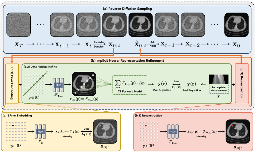
Figure 1: Overview of the proposed DPER. (a) The distribution prior sub-problem is addressed with reverse SDE sampling utilizing a pre-trained score model. At the sampling timestep $t$, the noiseless prior $\mathbf{x}_{0|t}$ is generated from $\mathbf{x}_{t}$ with Tweedie’s formula. Subsequently, $\mathbf{x}_{0|t}$ is refined with INR by solving the data fidelity subproblem (indicated by the orange arrow) to get $\hat{\mathbf{x}}_{0|t}$. Next, $\mathbf{x}_{t-1}$ is derived from $\hat{\mathbf{x}}_{0|t}$ by adding noise, enabling the continuation of the reverse SDE sampling. (b) The data fidelity sub-problem is addressed with an INR combing physical forward model of CT. First, the prior image $\mathbf{x}_{0|t}$ is embedded into an MLP network $\bm{\mathcal{F}}_{\mathbf{\Phi}}$. Then, we simulate the projections using the physical forward model of CT by sampling rays from the implicit representation. The parameters of $\bm{\mathcal{F}}_{\mathbf{\Phi}}$ is optimized by minimizing the distance between the predicted projection $\hat{\mathbf{y}}$ and the real projection $\mathbf{y}$. Finally, the refined prior image $\hat{\mathbf{x}}_{0|t}$ is generated from well-trained MLP $\bm{\mathcal{F}}_{\hat{\mathbf{\Phi}}}$.

3 Methodology

3.1 Overview

LACT and ultra-SVCT present highly under-determined inverse image reconstruction challenges. The image local consistency prior induced by INR hardly produces dependable solution space in such conditions [27, 20, 25]. In this study, we suggest integrating the diffusion model as a generative prior into the INR image reconstruction framework. The data distribution prior introduced by pre-trained score-based diffusion models serves as image regularization during the INR optimization process. This combination initially preserves the implicit image local consistency prior from INR. Additionally, it augments the feasibility of the solution space for the inverse problem through the diffusion model, resulting in increased stability and precision in the solutions.

Revisiting the ill-posed inverse problem as outlined in Eq. (2), if we reinterpret this issue within the framework of a diffusion model schema, it equates to resolving the Maximum A Posteriori (MAP) estimation problem at every timestep $t$:

$$\hat{\mathbf{x}_{t}}=\underset{\mathbf{x}}{\mathrm{arg}\min}\frac{1}{2\sigma^{2}}\left\|\mathbf{y}-\mathbf{A}\mathbf{x}_{t}\right\|^{2}+\lambda\cdot\mathcal{R}\left(\mathbf{x_{t}}\right),$$ (9)

To solve Eq. (9) more efficiently, a widely used approach is decoupling the data and prior terms using the split-variable method. We leverage the Half Quadratic Splitting (HQS) [41], it first introduces an auxiliary variable $\mathbf{z}$, and the Eq. (2) is equivalent to the constrained optimization problem as:

$$\hat{\mathbf{x}_{t}}=\underset{\mathbf{x}_{t}}{\mathrm{arg}\min}\frac{1}{2\sigma^{2}}\left\|\mathbf{y}-\mathbf{Ax}_{t}\right\|^{2}+\lambda\cdot\mathcal{R}\left(\mathbf{z}_{t}\right),\ \operatorname{s.t.}\ \mathbf{z}_{t}=\mathbf{x}_{t},$$ (10)

and Eq. (10) can be solved by minimizing the problem as follows:

$$\mathcal{L}_{\mu}\left(\mathbf{x},\mathbf{z}\right)=\frac{1}{2\sigma^{2}}\left\|\mathbf{y}-\mathbf{Ax}\right\|^{2}+\lambda\cdot\mathcal{R}\left(\mathbf{z}\right)+\frac{\mu}{2}\left\|\mathbf{z}-\mathbf{x}\right\|^{2},$$ (11)

where $\mu$ is a penalty parameter. The problem can be addressed by iteratively solving the following two subproblems while keeping the rest of the variables fixed:

$$\mathbf{x}_{t}=\underset{\mathbf{x}_{t}}{\mathrm{arg}\min}\left\|\mathbf{y}-\mathbf{A}\mathbf{x}_{t}\right\|^{2}+\mu\sigma_{i}^{2}\left\|\mathbf{x}-\mathbf{z}_{t-1}\right\|^{2}$$ (12a)

$$\mathbf{z}_{t}=\underset{\mathbf{z}_{t}}{\mathrm{arg}\min}\frac{1}{2(\sqrt{\lambda/\mu})^{2}}\left\|\mathbf{z}_{t}-\mathbf{x}_{t}\right\|^{2}+\mathcal{R}\left(\mathbf{z}_{t}\right),$$ (12b)

where Eq. (12a) defines the data-fidelity subproblem, concentrating on the identification of a proximal point in relation to $\mathbf{z}_{t-1}$. Meanwhile, the prior subproblem, as explicated in Eq. (12b), embodies a Gaussian denoising challenge, viewed through the lens of Bayesian analysis.

Firstly, we describe how to solve the prior subproblem (as Eq. (12b)) using the score-based diffusion model under the HQS framework as Eq. (12). This Gaussian denoising problem involves deriving a noise-free $\mathbf{z}_{t}$ from a noisy $\mathbf{x}_{t}$ (i.e., obtain the $\mathbf{x}_{0|t}$), where the noise level is quantified by $\sqrt{\lambda/\mu}$. In alignment with the approach adopted in [42], the noise schedule of our Variance Exploding Stochastic Differential Equation (VE-SDE) diffusion model is applied, setting $\sqrt{\lambda/\mu}=\sigma_{t}$. Furthermore, we introduce $\nabla_{\mathbf{x}}\mathcal{R}\left(\mathbf{x}\right)=-\nabla_{\mathbf{x}}\log p_{t}\left(\mathbf{x}\right)=-\mathbf{s}_{\bm{\theta}^{*}}(\mathbf{x}_{t},t)$, we can rewrite Eq. (12b) as:

$$\mathbf{z}_{t}=\mathbf{x}_{0|t}\approx\mathbf{x}_{t}+\sigma_{t}^{2}\mathbf{s}_{\bm{\theta}^{*}}\left(\mathbf{x}_{t},t\right),$$ (13)

which means that Eq. (12b) has been transformed into a Tweedie denoising process in VE-SDE diffusion schema. Then we can solve the data-fidelity subproblem to get a refined $\hat{\mathbf{x}}_{0|t}$ corrected with measurement $\mathbf{y}$. However, due to the highly undercharacterized nature of the problem, it is difficult to produce the desired result in a single iteration. To take full advantage of the multi-step sampling of the diffusion model, we follow [42] to add noise to the refined $\hat{\mathbf{x}}_{0|t}$ with noise level corresponding to timestep $t$. The operation mentioned above can be succinctly formulated as follows:

$${\mathbf{x}}_{t-1}=\hat{\mathbf{x}}_{0\mid t}+\sigma_{t-1}\bm{\epsilon},$$ (14)

which enables us to go back to the corresponding timestep of the diffusion model and continue sampling.

To illustrate our framework more clearly, we rewrite Eq. (12) as:

$$\mathbf{x}_{0|t}=\mathbf{x}_{t}+\sigma_{t}^{2}\mathbf{s}_{\bm{\theta}^{*}}\left(\mathbf{x}_{t},t\right),$$ (15a)

$$\hat{\mathbf{x}}_{0|t}=\underset{\mathbf{x}}{\mathrm{arg}\min}\left\|\mathbf{y}-\mathbf{A}\mathbf{x}\right\|^{2}+\mu\sigma_{i}^{2}\left\|\mathbf{x}-\mathbf{x}_{0|t}\right\|^{2},$$ (15b)

$${\mathbf{x}}_{t-1}=\hat{\mathbf{x}}_{0\mid t}+\sigma_{t-1}\bm{\epsilon},$$ (15c)

where Eq. (15b) denotes the prior subproblem, which estimates the noiseless image $\mathbf{x}_{0|t}$ via VE-SDE sampling with Tweedie’s formula. Eq. (15b) is the data-fidelity subproblem, and Eq. (15c) is the forward sampling operation by adding noise at timestep $t$.

For the data-fidelity subproblem as Eq. (15b), we employ INR to address it. The data-fidelity term $\left\|\mathbf{y}-\mathbf{A}\mathbf{x}\right\|^{2}$ ensures that the predicted $\mathbf{x}$ closely aligns with the measured data $\mathbf{y}$, thereby maintaining data fidelity. Additionally, the consistency term $\left\|\mathbf{x}-\mathbf{x}_{0|t}\right\|^{2}$ emphasizes the similarity of the predicted image $\mathbf{x}$ to the prior image $\mathbf{x}_{0|t}$, which serves to reduce artifacts that might arise from overfitting to incomplete measurements $\mathbf{y}$.

Fig. 1 shows the overview of the proposed DPER. In our approach, the distribution prior sub-problem is solved by the diffusion model as shown in Fig. 1(a). The image prior $\mathbf{x}_{T}$ is initially sampled from a Gaussian distribution $\mathcal{N}(0,1)$. Then, we generate a noisy prior image $\mathbf{x}_{t}$ at timestep $t$ by performing the reverse SDE process on a pre-trained score diffusion model. The generated noisy image $\mathbf{x}_{t}$ follows the pre-trained target distribution. Then we use Tweedie’s formula [43] to produce its denoised version $\mathbf{x}_{0\mid t}$, which serves as an initial solution to the distribution prior sub-problem (i.e., $\mathbf{z}_{k+1}=\mathbf{x}_{0\mid t}$ in Eq. (15a)). As demonstrated in Fig. 1(b), the initialized prior image $\mathbf{x}_{0\mid t}$ is subsequently transferred to the INR refinement phase to address the data fidelity sub-problem in Eq. (15b). In the prior embedding step (Fig. 1(b.1)), INR is initially trained to present $\mathbf{x}_{0\mid t}$. Then it is further refined towards the incomplete measurement $\mathbf{y}$ to generate a high fidelity and realistic solution as in Fig. 1(b.2). This refined image $\hat{\mathbf{x}}_{0\mid t}$ is the solution to the data fidelity sub-problem (i.e., $\mathbf{x}_{k+1}=\hat{\mathbf{x}}_{0\mid t}$ in Eq. (15b)). $\hat{\mathbf{x}}_{0\mid t}$ is then transferred back to the SDE process to further enhance the target distribution prior. By iteratively performing the reverse SDE sampling and INR refinement, the high-quality CT images can be reconstructed when the reverse SDE process is completed.

3.2 Generative Image Prior by Diffusion Model

We employ a score-based diffusion model of the ‘Variance Exploding (VE)’ SDE [44] form and utilize the reverse SDE sampling to address the distribution prior sub-problem in Eq. (15a). Specifically, the prior $\mathbf{x}_{T}$ is initialized with Gaussian distribution, and the denoising process based on score matching is executed sequentially with the timestep $T$ decay as follows:

$$\mathbf{x}_{t-1}=\mathbf{x}_{t}+\left(\sigma_{t}^{2}-\sigma_{t-1}^{2}\right)\mathbf{s}_{\bm{\theta}^{*}}\left(\mathbf{x}_{t},t\right)+\sqrt{\left(\sigma_{t}^{2}-\sigma_{t-1}^{2}\right)}\bm{\epsilon},$$ (16)

where $\bm{\epsilon}\sim\mathcal{N}(\mathbf{0},\mathbf{I})$, $\sigma_{t}$ is the noise scale at timestep $t$ and $\mathbf{s}_{\bm{\theta}^{*}}$ is the pre-trained score model.

When solving inverse problems via diffusion models, obtaining an estimated clean version of the sampled $\mathbf{x}_{t}$ before solving the data fidelity sub-problems has been shown to greatly improve performance [34, 45, 46, 47]. Tweedie’s formula [43] enables us to get the denoised result of $\mathbf{x}_{t}$ by computing the posterior expectation with one step, given a score function $\nabla_{\mathbf{x}_{t}}\log p\left(\mathbf{x}_{t}\right)$ as follows:

$$\mathbb{E}\left[\mathbf{x}_{0}\mid\mathbf{x}_{t}\right]=\mathbf{x}_{t}+\sigma_{t}^{2}\nabla_{\mathbf{x}_{t}}\log p\left(\mathbf{x}_{t}\right),$$ (17)

where $\sigma_{t}$ is the noise scale of $\mathbf{x}_{t}$. The expression is the same as the prior subproblem Eq. (15a) we derived in Sec. 3.1. Given the estimated score function provided by the pre-trained score model $\mathbf{s}_{\bm{\theta}^{*}}$, we employ Tweedie’s formula to get the noiseless prior image $\mathbf{x}_{0\mid t}$ from $\mathbf{x}_{t}$. $\mathbf{x}_{0\mid t}$ denotes the denoised result inferred from $\mathbf{x}_{t}$ for clarity and conciseness. The prior $\mathbf{x}_{0\mid t}$ is then employed to solve the data fidelity sub-problem with INR. The reverse SDE sampling corporating INR refinement to solve CT inverse problems can be rewritten specifically as:

$$\mathbf{x}_{0\mid{t}}=\mathbf{x}_{t}+\sigma_{t}^{2}\mathbf{s}_{\bm{\theta}^{*}}\left(\mathbf{x}_{t},t\right)$$ (18a)

$$\hat{\mathbf{x}}_{0\mid t}=\mathbf{INR}(\mathbf{x}_{0\mid t},\mathbf{y})$$ (18b)

$${\mathbf{x}}_{t-1}=\hat{\mathbf{x}}_{0\mid t}+\sigma_{t-1}\bm{\epsilon},$$ (18c)

where Eq. (18a) is the reverse diffusion sampling process with denoising by Tweedie’s formula, Eq. (18b) is the data fidelity sub-problem solving by INR (Sec. 3.3) and Eq. (18c) is the forward sampling operation by adding noise at timestep $t$.

3.3 Data Fidelity by Implicit Neural Representation

The data fidelity sub-problem in Eq. (15a) is addressed by the unsupervised deep learning architecture INR. Specifically, as shown in Fig. 1(b.2), we model the underlying CT image $\mathbf{x}$ as an implicit continuous function that maps image coordinates to intensities. Then CT imaging forward model is performed to simulate the physical acquisition process from the image $\mathbf{x}$ to its according projection measurements. By minimizing the errors on the measurement domain, we can optimize an MLP network $\mathcal{F}_{\mathbf{\Phi}}$ to approximate the implicit function of $\mathbf{x}$. The approximation of the implicit continuous function results in a highly accurate simulation of the CT imaging forward model, thereby ensuring effective data fidelity with the incomplete measurement $\mathbf{y}$.

When addressing the challenging issue of high underdetermination caused by LACT and ultra-SVCT, we propose to guide INR towards a solution that maintains data fidelity and avoids degradation by incorporating the generative prior $\mathbf{x}_{0\mid t}$ sampled by the diffusion model. Inspired by the INR work in [27], we solve the data fidelity sub-problem in three stages: 1) Prior Embedding, 2) Data Fidelity Refinement, and 3) Image Reconstruction.

3.3.1 Prior Embedding

In this stage, our goal is to incorporate the generative prior $\mathbf{x}_{0\mid t}$ from the diffusion model into the INR model. This strategy prevents INR from generating degradation reconstruction solution by avoiding overfitting to incomplete measurements $\mathbf{y}$. Technically, we represent the prior image $\mathbf{x}_{0\mid t}$ as a continuous function of image coordinate, which can be expressed as below:

$$f:\mathbf{p}=(x,y)\in\mathbb{R}^{2}\rightarrow\mathbf{x}_{0\mid t}(\mathbf{p})\in\mathbb{R},$$ (19)

where $\mathbf{p}$ is any spatial coordinate and $\mathbf{x}_{0\mid t}(\mathbf{p})$ is the corresponding intensity of the prior image at that position. As illustrated in Fig. 1(b.1), we leverage an MLP network $\mathcal{F}_{\mathbf{\Phi}}$ to approximate the function $f$ through optimizing the following objective function:

$$\mathbf{\Phi}_{\mathrm{prior}}=\underset{\mathbf{\Phi}}{\mathrm{arg}\min}\frac{1}{N}\sum_{i=1}^{N}{\left\|\mathcal{F}_{\mathbf{\Phi}}\left(\mathbf{p}_{i}\right)-\mathbf{x}_{0\mid t}\left(\mathbf{p}_{i}\right)\right\|^{2}},$$ (20)

where $N$ denotes the number of sampling image coordinates at each iteration, $\mathbf{p}_{i}$ denotes the $i^{th}$ spatial coordinate. Once the optimization is completed, the prior image $\mathbf{x}_{0\mid t}(\mathbf{p})$ is embedded into the trainable weight $\mathbf{\Phi}_{\mathrm{prior}}$ of the MLP network. From the initialization perspective, we construct a feasible initialization that follows the target distribution for INR model using the generative prior provided by diffusion model. From an initialization standpoint, we establish a viable starting point for the INR model, utilizing the generative prior offered by the diffusion model.

3.3.2 Data Fidelity Refinement

After the prior embedding, the INR network $\mathcal{F}_{\mathbf{\Phi}_{\mathrm{prior}}}$ incorporates the prior image $\mathbf{x}_{0\mid t}$. However, this prior image lacks data fidelity to the real incomplete measurement $\mathbf{y}$ since it is generated through unconditional random sampling. Therefore, we need to refine the MLP network $\mathcal{F}_{\mathbf{\Phi}_{\mathrm{prior}}}$ towards the measurement $\mathbf{y}$ by integrating the CT imaging model. Fig. 1(b.2) shows the refinement process. Technically, we sample coordinates $\mathbf{p}$ at a fixed interval $\Delta\mathbf{p}$ along an X-ray $\mathbf{r}$ and feed these coordinates into the MLP network to produce the corresponding intensities $I=\mathcal{F}_{\mathbf{\Phi}_{\mathrm{prior}}}(\mathbf{p})$. Then, we perform the CT imaging forward model (i.e., line integral transform) to generate the according measurement $\hat{\mathbf{y}}(\mathbf{r})$ for the X-ray $\mathbf{r}$. Finally, the MLP network $\mathcal{F}_{\mathbf{\Phi}_{\mathrm{prior}}}$ can be refined by minimizing the distance between the estimated measurement $\hat{\mathbf{y}}$ and real measurement $\mathbf{y}$. Formally, this process can be expressed as below:

$$\mathbf{\Phi}_{\mathrm{refine}} =\underset{\mathbf{\Phi}_{\mathrm{prior}}}{\mathrm{arg}\min}\frac{1}{|\mathcal{R}|}\sum_{\mathbf{r}\in\mathcal{R}}|\hat{\mathbf{y}}(\mathbf{r})-\mathbf{y}(\mathbf{r})|,$$ (21)

$$\hat{\mathbf{y}}(\mathbf{r}) =\sum_{\mathbf{p}\in\mathbf{r}}\mathcal{F}_{\mathbf{\Phi}_{\mathrm{prior}}}(\mathbf{p})\cdot\Delta\mathbf{p},$$

where $\mathcal{R}$ denotes a set of sampling X-rays $\mathbf{r}$ at each iteration.

3.3.3 Image Reconstruction

Once the data fidelity refinement is completed, the MLP network $\mathcal{F}_{\mathbf{\Phi}_{\mathrm{refine}}}$ represents a solution $\hat{\mathbf{x}}_{0\mid t}$ that inherits the generative prior $\mathbf{x}_{0\mid t}$ from the diffusion model and is also highly consistent with the actual measurements $\mathbf{y}$. Then, we reconstruct the solution $\hat{\mathbf{x}}_{0\mid t}(\mathbf{p})$ by feeding necessary image coordinates $\mathbf{p}$ into the MLP network $\mathcal{F}_{\mathbf{\Phi}_{\mathrm{refine}}}$, i.e., $\hat{\mathbf{x}}_{0\mid t}=\mathcal{F}_{\mathbf{\Phi}_{\mathrm{refine}}}(\mathbf{p})$.

Algorithm 1 DPER

1:Measurements $\mathbf{y}$, Pre-trained score function $\mathbf{s}_{\bm{\theta}^{*}}$, MLP network $\mathcal{F}_{\mathbf{\Phi}}$, Timesteps $T$, Refinement interval RI, Noise schedule $\{\sigma_{t}\}_{t=0}^{T}$, Coordinates of target images $\mathbf{p}$, Sampled X-rays set $\mathcal{R}$.

2:$\mathbf{x}_{T}\sim({\bf 0},\sigma_{T}^{2}\mathbf{I})$;

3:for $t=T,\dots,1$ do

4:     $\triangleright$ 1. Distribution Prior Sub-problem

5:     $\bm{\epsilon}\thicksim\mathcal{N}\,\,(\mathbf{0},\mathbf{I})$

6:     $\mathbf{x}_{t-1}=\mathbf{x}_{t}+\left(\sigma_{t}^{2}-\sigma_{t-1}^{2}\right)\mathbf{s}_{\bm{\theta}^{*}}\left(\mathbf{x}_{t},t\right)+\sqrt{\left(\sigma_{t}^{2}-\sigma_{t-1}^{2}\right)}\bm{\epsilon}$

7:     if $(t-1)\ \mathrm{mod}\ \texttt{RI}=0$ then

8:         $\mathbf{x}_{0\mid t}=\mathbf{x}_{t}+\sigma_{t}^{2}\mathbf{s}_{\bm{\theta}^{*}}\left(\mathbf{x}_{t},t\right)$ $\triangleright$ Tweedie’s formula

9:         $\triangleright$ 2. Data Fidelity Sub-problem

10:         $\mathbf{\Phi}_{\mathrm{prior}}=\underset{\mathbf{\Phi}}{\mathrm{arg}\min}\frac{1}{N}\sum_{i=1}^{N}{\left\|\mathcal{F}_{\mathbf{\Phi}}\left(\mathbf{p}\right)-\mathbf{x}_{0\mid t}\left(\mathbf{p}\right)\right\|^{2}}$

11:         $\mathbf{\Phi}_{\mathrm{refine}}=\underset{\mathbf{\Phi}_{\mathrm{prior}}}{\mathrm{arg}\min}\frac{1}{|\mathcal{R}|}\sum_{\mathbf{r}\in\mathcal{R}}|\hat{\mathbf{y}}(\mathbf{r})-\mathbf{y}(\mathbf{r})|$

12:         $\hat{\mathbf{x}}_{0\mid t}=\mathcal{F}_{\mathbf{\Phi}_{\mathrm{refine}}}(\mathbf{p})$

13:         ${\mathbf{x}}_{t-1}=\hat{\mathbf{x}}_{0\mid t}+\sigma_{t-1}\bm{\epsilon}$, $\bm{\epsilon}\thicksim\mathcal{N}\,\,(\mathbf{0},\mathbf{I})$ $\triangleright$ Add Noise

14:     end if

15:end for

16:return $\mathbf{x}_{0}$

3.4 Alternative Optimization Strategy

Following the HQS algorithm, we iteratively optimize the diffusion model-based regularization sub-problem and the INR-based data fidelity sub-problem using an alternative approach. As shown in Algorithm 1, we intersperse the solution of the data fidelity sub-problem with the reverse SDE sampling process (as distribution prior sub-problem). A hyper-parameter refinement interval $\texttt{RI}\in\mathbb{R}$ is introduced for balancing the weights of the two sub-problems in the overall process. RI enables the data fidelity sub-problem to be executed at a specified time step. When $(t-1)\mod\texttt{RI}\neq 0$, our algorithm solely performs reverse SDE denoising to generate images that match the target distribution, i.e., solving the distribution prior sub-problem. When $(t-1)\mod\texttt{RI}=0$, we solve the data fidelity sub-problem once at the current timestep. Specifically, an estimated clean image at $t$ is obtained using Eq. (18a). Then, INR is applied to optimize the data fidelity sub-problem given the measurement $\mathbf{y}$ and prior image ${\mathbf{x}}_{0\mid t}$, as explained in Sec. 3.3. Finally, the corresponding level of noise is added to the result $\hat{\mathbf{x}}_{0\mid t}$ to return to the manifold at timestep $t-1$ and continue back to the reverse SDE sampling. We can trade-off between reconstruction performance and computational consumption by tuning the RI as discussed in Sec. 4.5.

3.5 Implementation Details

For the Diffusion Sampling stage (Fig. 1(a)), we set the total number of the sampling $T$ as 2000 and the refinement interval RI as 50. We adopt the ncsnpp [44] network as the score-based diffusion model architecture without any modification. For the INR refinement stage (Fig. 1(b)), we combine hash encoding [40] with five fully connected (FC) layers of 128 width to implement the MLP network $\mathcal{F}_{\Phi}$. The ReLU function is applied in each hidden layer. Hash encoding is a method which stores the trainable feature vectors in different multi-resolution hash tables to map the low-dimensional input to a higher dimensional space and thus enable network to efficiently learn higher frequency image feature. The hyper-parameters of the hash encoding are as follow: $L=10$, $T=2^{23}$, $F=8$, $N_{\text{min}}=2$, and $b=2$. During the prior embedding and data fidelity refinement, the numbers of training iterations are 50 and 250, the batch sizes are 1000 (i.e., $N=1000$ in Eq. (20)) and 128 (i.e., $|\mathcal{R}|=128$ in Eq. (21)), and the learning rates are 1e-3 and 1e-4. Adam optimizer with default hyper-parameters is leveraged. Note that all hyper-parameters are tuned on two samples of the AAPM dataset [48] and are then held constant across all other samples.

4 Experiments

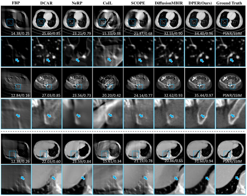
Figure 2: Qualitative results of methods in comparison on two test samples (#0 (Rows 1-2), #239 (Rows 3-4) of the AAPM dataset and #1 (Rows 5-6)) of the LIDC dataset for the LACT task of [0, 90]° scanning range.

Table 1: Quantitative results of methods in comparison on the AAPM and LIDC datasets for the LACT tasks of [0, 90]°, [0, 120]°, and [0, 150]° scanning ranges. The best and second best results are highlighted in bold and underline, respectively.

Dataset	Method	[0, 90]°		[0, 120]°		[0, 150]°
		PSNR$\uparrow$	SSIM$\uparrow$	PSNR$\uparrow$	SSIM$\uparrow$	PSNR$\uparrow$	SSIM$\uparrow$
AAPM	FBP[49]	13.73$\pm$0.52	0.3015$\pm$0.0419	16.97$\pm$0.63	0.3995$\pm$0.0350	22.41$\pm$1.25	0.5002$\pm$0.0353
	DCAR[16]	28.27$\pm$1.39	0.8796$\pm$0.0180	34.36$\pm$1.60	0.9426$\pm$0.0108	38.69$\pm$1.05	0.9658$\pm$0.0086
	DDNet[13]	26.85$\pm$1.43	0.7342$\pm$0.0300	31.00$\pm$1.54	0.8259$\pm$0.0265	34.92$\pm$1.50	0.8812$\pm$0.0211
	NeRP[27]	24.34$\pm$2.05	0.7511$\pm$0.0626	31.96$\pm$3.19	0.9077$\pm$0.0354	36.98$\pm$3.07	0.9441$\pm$0.0260
	CoIL[25]	18.44$\pm$1.62	0.4002$\pm$0.0521	20.99$\pm$1.85	0.5398$\pm$0.0409	28.40$\pm$1.95	0.7936$\pm$0.0484
	SCOPE[20]	23.77$\pm$1.98	0.8079$\pm$0.0306	30.45$\pm$2.72	0.9312$\pm$0.0161	37.67$\pm$1.46	0.9752$\pm$0.0039
	MCG[34]	32.66$\pm$2.35	0.9306$\pm$0.0120	34.93$\pm$1.41	0.9445$\pm$0.0065	35.78$\pm$0.78	0.9486$\pm$0.0063
	DiffusionMBIR[35]	35.07$\pm$2.26	0.9483$\pm$0.0084	37.21$\pm$2.92	0.9660$\pm$0.0057	42.34$\pm$0.82	0.9802$\pm$0.0063
	DPER (Ours)	37.20$\pm$2.38	0.9759$\pm$0.0064	43.17$\pm$1.91	0.9902$\pm$0.0027	50.01$\pm$1.30	0.9978$\pm$0.0015
LIDC	FBP[49]	12.79$\pm$0.94	0.2753$\pm$0.0273	15.71$\pm$1.02	0.4508$\pm$0.0338	19.02$\pm$1.23	0.5614$\pm$0.0465
	DCAR[16]	20.84$\pm$1.50	0.5909$\pm$0.0487	24.29$\pm$1.78	0.6867$\pm$0.0522	27.76$\pm$1.87	0.7465$\pm$0.0536
	DDNet[13]	20.20$\pm$1.65	0.5951$\pm$0.0425	24.31$\pm$1.48	0.7066$\pm$0.0464	27.66$\pm$1.31	0.7419$\pm$0.0527
	NeRP[27]	22.53$\pm$1.00	0.7163$\pm$0.0194	26.37$\pm$1.89	0.8128$\pm$0.0303	31.32$\pm$1.14	0.8723$\pm$0.0168
	CoIL[25]	15.93$\pm$0.59	0.3619$\pm$0.0493	17.03$\pm$0.96	0.4520$\pm$0.0438	22.76$\pm$1.55	0.6142$\pm$0.0389
	SCOPE[20]	19.67$\pm$1.13	0.6456$\pm$0.0358	26.92$\pm$1.58	0.8785$\pm$0.0307	38.36$\pm$1.75	0.9818$\pm$0.0073
	MCG[34]	21.58$\pm$1.01	0.7910$\pm$0.0189	24.64$\pm$2.51	0.8623$\pm$0.0341	32.52$\pm$2.03	0.9296$\pm$0.0177
	DiffusionMBIR[35]	23.27$\pm$1.47	0.8197$\pm$0.0278	28.93$\pm$1.68	0.9170$\pm$0.0215	35.67$\pm$1.69	0.9548$\pm$0.0125
	DPER (Ours)	28.96$\pm$1.29	0.9134$\pm$0.0223	34.76$\pm$1.72	0.9655$\pm$0.0092	42.42$\pm$1.86	0.9882$\pm$0.0041

4.1 Experimental Settings

4.1.1 Dataset and Pre-Processing

We conduct experiments on two well-known public CT datasets, including AAPM 2016 low-dose CT grand challenge [48] and Lung Image Database Consortium (LIDC) image collection dataset [50]. The AAPM dataset DICOM Full Dose data was acquired at 120kV and 200mAs in the portal venous phase using a Siemens SOMATOM Flash scanner. For the acquired cone-beam projections, we approximated them to fan beam geometry using helix2fan, and then all volumes were reconstructed via standard filtered back projection (FBP). The LIDC database is not performed specifically for the purpose of the database so a heterogeneous range of scanner models (e.g., GE Medical Systems LightSpeed scanner models, Toshiba Aquilion scanners, Philips Brilliance scanner models) and technical parameters (e.g., 120-140kV tube peak potential energies, 40-627 mA tube current range, 0.6mm-5.0mm slice thickness) were represented. There are evident differences in the acquisition protocol and subjects between LIDC and AAPM datasets. Therefore, the evaluation based on the LIDC dataset can effectively reflect the generalization and robustness of the reconstruction methods in OOD settings. For the AAPM dataset, we extract 5376 2D slices from CT volumes of 9 subjects and randomly split them into 4240 training slices and 1136 validation slices. We then use 101 slices from an unseen volume as test data. For the LIDC dataset, we randomly choose 9 slices from various subjects as additional test data. Moreover, we retrospectively employ radon transform implemented by scikit-image library of Python (i.e., parallel X-ray beam) to generate the incomplete (SV and LA) projection data. Note that the training and validation images from only the AAPM dataset are used for training three supervised baselines (FBPConvNet, DCAR, and DDNet).

We also conduct experimental validation on an in-house COVID-19 chest clinical CT dataset. All subjects were patients with severe COVID-19 who underwent serial chest CT scans during hospital stay. The examinations were performed with an Optima CT680 CT scanner (GE Medical Systems, USA;). The CT protocol was as follows: the tube voltage was 120 kVp, X-ray tube current was automatic (180$\sim$400 mA). The distance between the source and the detector was 94.9 cm, and the distance between the source and patient was 54.1 cm, respectively. The image matrix featured dimensions of 512$\times$512 pixels. The LACT and SVCT projections were extracted from the rebind fan-beam full-view projection data. To validate the robustness and performance of our method, we seamlessly applied the score function trained on the AAPM dataset to clinical data. It is worth noting that our score function was trained on 256$\times$256 images, so we generated a reconstruction of the same size and resized the reference image accordingly to compute the metrics.

4.1.2 Methods in comparison

Eight representative CT reconstruction approaches from three categories are utilized as comparative methods: 1) one model-based method (FBP [49]); 2) three supervised CNN-based DL methods (FBPConvNet [11], DDNet [13], and DCAR [16]); 3) Five unsupervised DL methods (SCOPE [20], NeRP [27], CoIL [25], MCG [34] and DiffusionMBIR [35]). Among them, FBPConvNet is solely utilized for the SVCT task, while DCAR is exclusively applied to the LACT task. We implement the three supervised methods according to the original papers and subsequently train them on the training and validation sets of the AAPM dataset using the Adam optimizer [51] with a mini-batch size of 16 and a learning rate of 1e-4. The training epochs for FBPConvNet and DCAR are set to 50, while for DDNet, it is set to 500. It is important to emphasize that these hyperparameters have been meticulously fine-tuned on the AAPM dataset to ensure a fair comparison. As for the five fully unsupervised methods (SCOPE, NeRP, CoIL, MCG, and DiffusionMBIR) are evaluated using their official code. As diffusion-based models, MCG, DiffusionMBIR, and our DPER use the same score function checkpoint provided by Chung et al. [35], which is pre-trained on the AAPM dataset. For the three fully unsupervised INR-based methods, we carefully tune their hyper-parameters on two samples from the AAPM datasets and then fix these parameters for all other cases.

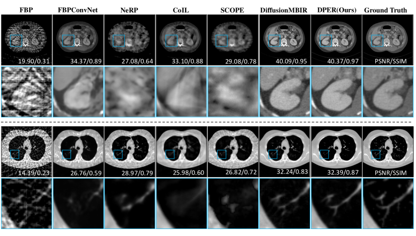
Figure 3: Qualitative results of methods in comparison on two test samples (#133 (Rows 1-2) and #1 (Rows 3-4)) of the AAPM and LIDC datasets for the ultra-SVCT task of 20 input views.

Table 2: Quantitative results of methods in comparison on the AAPM and LIDC datasets for the ultra-SVCT tasks of 10, 20, and 30 input views. The best and second best results are highlighted in bold and underline, respectively.

Dataset	Method	10 views		20 views		30 views
		PSNR$\uparrow$	SSIM$\uparrow$	PSNR$\uparrow$	SSIM$\uparrow$	PSNR$\uparrow$	SSIM$\uparrow$
AAPM	FBP[49]	13.54$\pm$0.71	0.1725$\pm$0.0082	18.78$\pm$0.86	0.2993$\pm$0.0162	22.63$\pm$3.24	0.4107$\pm$0.0233
	FBPConvNet[11]	28.56$\pm$1.01	0.7950$\pm$0.0292	32.84$\pm$1.19	0.8751$\pm$0.0225	35.29$\pm$1.33	0.9127$\pm$0.0201
	DDNet[13]	26.54$\pm$0.91	0.7005$\pm$0.0277	30.43$\pm$0.97	0.7905$\pm$0.0214	32.82$\pm$1.29	0.8516$\pm$0.0232
	NeRP[27]	19.63$\pm$2.35	0.3864$\pm$0.0843	25.67$\pm$1.52	0.6139$\pm$0.0597	29.98$\pm$1.47	0.7694$\pm$0.0456
	CoIL[25]	25.46$\pm$1.00	0.6841$\pm$0.0363	31.62$\pm$1.32	0.8563$\pm$0.0220	34.74$\pm$1.32	0.9099$\pm$0.0147
	SCOPE[20]	22.13$\pm$0.67	0.5525$\pm$0.0287	28.10$\pm$0.70	0.8249$\pm$0.0135	32.22$\pm$1.19	0.8596$\pm$0.0190
	MCG[34]	34.27$\pm$0.65	0.9202$\pm$0.0094	35.22$\pm$0.57	0.9327$\pm$0.0084	35.62$\pm$0.56	0.9384$\pm$0.0086
	DiffusionMBIR[35]	37.20$\pm$1.26	0.9531$\pm$0.0065	39.88$\pm$1.03	0.9651$\pm$0.0054	40.78$\pm$0.80	0.9694$\pm$0.0044
	DPER (Ours)	37.05$\pm$1.71	0.9587$\pm$0.0081	40.33$\pm$1.23	0.9722$\pm$0.0048	42.32$\pm$0.94	0.9846$\pm$0.0035
LIDC	FBP[49]	10.20$\pm$1.09	0.1306$\pm$0.0207	15.30$\pm$0.90	0.2417$\pm$0.0303	18.52$\pm$0.83	0.3363$\pm$0.0375
	FBPConvNet[11]	22.37$\pm$1.02	0.4623$\pm$0.0369	26.37$\pm$0.98	0.6081$\pm$0.3115	29.23$\pm$0.85	0.7417$\pm$0.0235
	DDNet[13]	21.45$\pm$1.14	0.5209$\pm$0.0477	25.21$\pm$0.96	0.6238$\pm$0.0441	26.50$\pm$1.51	0.6809$\pm$0.0358
	NeRP[27]	17.95$\pm$1.99	0.4894$\pm$0.0482	26.09$\pm$1.39	0.7327$\pm$0.0313	30.15$\pm$1.29	0.8299$\pm$0.0291
	CoIL[25]	21.15$\pm$0.72	0.5209$\pm$0.0477	25.62$\pm$0.86	0.6270$\pm$0.0261	27.61$\pm$0.75	0.7251$\pm$0.0214
	SCOPE[20]	22.28$\pm$0.69	0.6157$\pm$0.0498	26.87$\pm$0.89	0.7412$\pm$0.0436	29.56$\pm$1.14	0.8119$\pm$0.0424
	MCG[34]	26.24$\pm$1.04	0.7679$\pm$0.0367	30.31$\pm$1.15	0.8623$\pm$0.0225	32.28$\pm$1.09	0.8897$\pm$0.0263
	DiffusionMBIR[35]	26.75$\pm$0.57	0.8081$\pm$0.0306	31.04$\pm$1.02	0.8782$\pm$0.0286	33.48$\pm$1.19	0.9120$\pm$0.0221
	DPER (Ours)	27.20$\pm$1.21	0.8318$\pm$0.0344	31.67$\pm$1.30	0.9005$\pm$0.0255	34.39$\pm$1.32	0.9321$\pm$0.0197

4.1.3 Evaluation Metrics

We utilize two standard metrics to quantitatively assess the performance of the compared methods: Peak Signal-to-Noise Ratio (PSNR) and Structural Similarity Index Measure (SSIM).

4.2 Comparison with SOTA Methods for LACT Task

We compare the proposed DPER model with the eight baselines on the AAPM and LIDC datasets for the LACT reconstructions with scanning angles of [0, 90]°, [0, 120]°, and [0, 150]° scanning ranges. Table 1 shows the quantitative results. On the AAPM dataset, our DPER, DiffusionMBIR and MCG produce the top-three performances and are significantly superior to the other baselines, benefiting from the generative prior provided by the diffusion model. However, on the LIDC dataset, we observe that DiffusionMBIR and MCG, trained on the AAPM dataset, experience severe performance degradation due to the out-of-distribution (OOD) problem. In some cases, their results were even worse than naive INR-based SCOPE, for example, 35.67 dB compared to 38.36 dB in PSNR for the [0, 150]° range. In contrast, the performance of our method remains stable over two different test datasets. Compared with DiffusionMBIR and MCG, DPER achieves superior results for the demanding OOD LIDC dataset by utilizing the INR method, which guarantees dependable data fidelity with the CT measurement data while maintaining the prior local image consistency.

Fig. 2 demonstrates the qualitative results on two representative samples (#0 and #1) from the AAPM and LIDC datasets. Upon visual inspection, it is evident that the model-based FBP and three INR-based methods (NePR, CoIL, and SCOPE) fail to yield satisfactory results on either dataset. This limitation is primarily attributed to the significant data gap inherent in the LACT problem. Although DCAR and DiffusionMBIR produce satisfactory results on the AAPM dataset, their reconstructions on the LIDC dataset exhibit noticeable distortions, primarily attributed to the out-of-distribution (OOD) problem. Conversely, the CT images generated by our DPER model across both datasets demonstrate high image quality in terms of both local details and global structural integrity.

4.3 Comparison with SOTA Methods for Ultra-SVCT Task

Additionally, we conduct a comparative evaluation of our DPER model against eight baseline methods on the AAPM and LIDC datasets for ultra-SVCT reconstructions with 10, 20, and 30 input views. We present the quantitative results in Table 2. The three INR-based methods hardly produce pleasing results for the ultra-SVCT task. Supervised FBPConvNet and DDNet perform well on the AAPM dataset while suffering from severe performance drops on the out-of-distribution LIDC dataset. DPER, DiffusionMBIR and MCG all obtain excellent and robust results on two datasets.

Fig. 3 shows the qualitative result on two representative samples (#133 and #1) of AAPM and LIDC datasets. The results from the FBP algorithm suffer severe streaking artifacts, while INR-based methods (NeRP, CoIL, and SCOPE) produce overly smooth artifacts results. INR-based methods tend to overfit the incomplete measurement and lack data distribution prior information, resulting in less detailed tissue reconstruction compared to the supervised method FBPConvNet. FBPConvNet yields relatively acceptable results. However, the structure precision remains somewhat unclear. In the ultra-SVCT task, DPER and DiffusionMBIR obtain the best and second-best performance (Except for 10 views, DPER gets second-best PSNR and best SSIM). Compared to DiffusionMBIR, our DPER achieves comparable performance on the AAPM dataset, while on out-of-distribution LIDC data, we slightly outperform in data consistency and performance. The findings from LIDC show that the three diffusion-based methods produce favorable reconstruction results, even when dealing with out-of-distribution data in the ultra-SVCT task.

4.4 Clinical Dataset Results

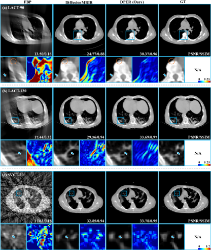
Figure 4: Comparison of LACT task (a. [0, 90]° and b. [0, 120]°) and SVCT task (c. 20 views) on test samples (#90, #178 and #213) of the clinical COVID-19 CT dataset.

Table 3: Quantitative results (PSNR / SSIM) of different methods on the clinical COVID-19 CT dataset for LACT task (90° and 120°) and SVCT task (20 views). The Best performances are highlighted in bold.

Method	LACT		SVCT
	[0, 90]°	[0, 120]°	20 views
FBP	12.01 / 0.2370	14.48 / 0.2788	11.51 / 0.1492
DiffusionMBIR [35]	26.01 / 0.8815	28.54 / 0.9192	30.96 / 0.9119
DPER	31.63 / 0.9548	33.07 / 0.9678	31.92 / 0.9286

To conduct a further comprehensive assessment on the effectiveness of our method, we undertaken experimental validation on the clinical COVID-19 CT dataset. We compared the proposed DPER with the current state-of-the-art method DiffusionMBIR on LACT task (with 90° and 120° scanning, respectively) and SVCT task (with 20 views projection).

Fig. 4 shows the qualitative results on some samples (#90, #178 and #213) of the clinical COVID-19 CT dataset. Confronted with this challenging OOD scenario (different acquisition protocols, anomalous structures caused by diseases), the proposed DPER consistently demonstrates commendable generalization performance. As depicted in Fig. 4(a), for the 90° LACT task, our DPER significantly outperforms the SOTA method DiffusionMBIR, both in quantitative metrics and visual representation. Specifically, in areas highlighted by orange circles and blue arrows, the reconstruction results from DiffusionMBIR either omit or distort the original bone structure. In contrast, the results obtained from DPER closely align with the ground truth. This is further corroborated by the 120° LACT task results, as illustrated in Fig. 4(b). In situations involving anomalous structures attributable to COVID-19, our DPER method demonstrated a notable capability to recover the original content of these structures to the greatest extent possible. In contrast, the DiffusionMBIR method exhibited blurring and inaccuracies in reconstructing these anomalous areas. In summary, DPER can still hold outstanding performance in the more complex out-of-distribution clinical dataset without any fine-tuning on pre-trained diffusion prior.

4.5 Effectiveness of Refinement Interval

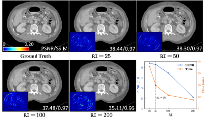
Figure 5: Qualitative and quantitative results of the DPER with five different refinement intervals RI on a test sample (#133) of the AAPM dataset for the LACT task of [0, 90]° scanning range.

In the proposed framework, the hyperparameter refinement interval RI balances the contribution of the data fidelity sub-problem and the distribution prior sub-problem in Eq. (15). To evaluate its impact, we set four distinct RI values (25, 50, 100, and 200) on the AAPM dataset for the LACT task with the scanning range of [0, 90]°. Fig. 5 shows the model performance and time cost curve varying with the refinement interval and the qualitative comparisons. It is clear that as the refinement interval increases, the performance of the model gradually decreases, but the running time of the model increases considerably. As the refinement interval increases, the influence of the distribution prior regularization becomes more pronounced in the solution of the overall inverse problem, while the impact of the data fidelity subproblem diminishes. Thereby, the reconstructed image may be divergent from GT. The visualization results are consistent with the quantitative analysis. In short, refinement intervals provide us with a balanced choice between performance and time consumption. It is worth noting that when the $\texttt{RI}\leqslant 50$, further reduction of the refinement interval results in a very limited performance gain (e.g., only 0.14 improvement in PSNR) but a multiplicative computational cost. Therefore, in this paper we set $\texttt{RI}=50$.

4.6 Comparison of MBIR and INR as Data-fidelity Solver

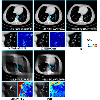
Figure 6: Qualitative and quantitative results of MBIR (ADMM-TV) and INR with/without score-based function(DiffusionMBIR is ADMM-TV with score-based function, DPER is INR with score-based function) on one test sample(# 8)) of the AAPM dataset for the LACT task of [0, 90]° scanning range.

To explore the advantages of the proposed DPER in solving the data-fidelity subproblem as Eq. (15b), we evaluate the performance of traditional MBIR and INR-based methods under two distinct scenarios: one involving the application of a diffusion model as a prior augmentation, and the other without it. Specifically, ADMM-TV and SCOPE have been selected as prototypical examples of MBIR and INR-based methods, respectively. Furthermore, DiffusionMBIR and proposed DPER are employed as representatives of the two methods in the case with diffusion prior. Fig. 6 displays example results for the LACT task with a scanning range of [0, 90]°. In the absence of a diffusion prior, the MBIR method tends to exhibit vast divergence phenomenon in tissue edges or boundaries, rendering fine structures challenging to discern. Conversely, owing to the inherent continuity prior, INR-based methods demonstrate a marked efficacy in constraining the solution space for the data-fidelity subproblem. This is particularly noticeable in regions that are not directly visible and in the delineation of fine structures. With the introduction of the diffusion prior, this advantage is directly reflected in a better solution for the data-fidelity subproblem (i.e., Eq. (15b)) in the overall framework as Eq. (15). Additionally, the reconstruction results and error map show that the INR provides a higher data fidelity than ADMM-TV, which leads the DPER to hold a better authenticity than DiffusionMBIR in the detailed area.

4.7 Effectiveness of Tweedie Denoising

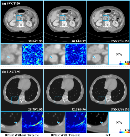
Figure 7: Comparison of LACT task of [0, 90]° and SVCT task of 20 views with and without Tweedie denoising in the proposed DPER.

To fully illustrate the benefits of Tweedie’s strategy for $\mathbf{x}_{0}$ estimation, we conducted ablation experiments to compare the difference between using $\mathbf{x}_{0}$ (i.e., $\left\|\mathbf{A}\hat{\mathbf{x}}_{0|t}-\mathbf{y}\right\|_{2}^{2}$) and $\mathbf{x}_{t}$ (i.e., $\left\|\mathbf{A}{\mathbf{x}}_{t}-\mathbf{y}\right\|_{2}^{2}$ for solving the data-fidelity subproblem. Fig. 7 displays the qualitative results of these two schemes on the AAPM dataset of the LACT task of [0, 90]° scanning range and SVCT task of 20 views. In the SVCT task, the reconstruction results of DPER without Tweedie denoising exhibit significant blur (as shown in the zoomed-in area of Fig. 7(a)). These results are characterized by indistinct boundaries between tissues and the presence of noticeable noise, which compromises the clarity and distinctness of the reconstructed images. In contrast, the reconstruction of DPER with Tweedie denoising is much clearer. The 90° LACT task shows a similar phenomenon; for example, in Fig. 7(b), the blue arrow indicates that Tweedie denoising provides more precise information. DPER with Tweedie outperforms DPER without Tweedie in both LACT and SVCT tasks. Recently, a lot of work has been demonstrating that using Tweedie denoising helps improve the performance of solving inverse problems via diffusion model [34, 47]. Indeed, using estimated $\mathbf{x}_{0}$ for data consistency operations (i.e., $\left\|\mathbf{A}\hat{\mathbf{x}}_{0|t}-\mathbf{y}\right\|_{2}^{2}$)) has become a widely used and recognized paradigm in the field of solving inverse problems via diffusion model [34, 47, 46, 42].

4.8 Effectiveness of Alternating Optimization Strategy

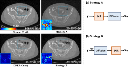
Figure 8: Qualitative results of different strategies on a test sample (#276) of the AAPM dataset for the LACT task of [0, 90]° scanning range. The right side shows the flowchart of strategies A and B.

To evaluate the effectiveness of alternative optimization, we compared two naive strategies (as shown in Fig. 8) that directly integrate the INR and diffusion model [52, 53] without alternative optimization of the proposed framework. Strategy A: INR first represents the implicit representation field by fitting the incomplete measurement directly. Then, the pre-trained diffusion model performs conditional sampling to refine the represented field to produce the reconstruction result. Strategy B: First, the pre-trained diffusion model performs conditional sampling based on the FBP result of the incomplete measurement. Then, the generated result is refined by INR (followed by the Implicit Neural Representation Refinement process of DPER) to produce the reconstruction result. Conditional sampling is performed by incorporating the input image and the according level noise.

Fig. 8 shows the performance of the proposed alternate optimization outperforms strategies A and B. From the error map, the reconstructed result of strategy A is greatly different from ground truth, which can be caused by insufficient data fidelity constraints in generating. In contrast, strategy B achieves improved data fidelity but retains some artifacts. DPER with an alternative optimization strategy yields accurate and high-fidelity reconstructed results. This suggests that the alternative optimization effectively balances the prior and data fidelity terms, leading to high-fidelity results in CT reconstruction.

4.9 Evaluating Robustness of the Reconstruction

4.9.1 The uncertainty of reconstruction

Due to the generative nature of diffusion models, DPER can produce multiple feasible reconstructed results with slightly different results based on the same incomplete measurement. To evaluate the robustness and qualify the uncertainty of reconstructions, we perform ten reconstructions simultaneously on the same incomplete measurements and calculate the mean and standard deviation of the reconstructions. In Fig. 9, the mean of reconstructions is close to ground truth. In the standard deviation map, the portion with actual measurements has a lower value, which proves that the INR refinement provides efficient data fidelity constraint in reconstruction. In conclusion, DPER can reduce the uncertainty of reconstruction, which can provide reliable results.

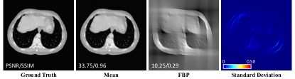
Figure 9: Qualitative results of quantifying uncertainty of reconstruction on a test sample (#40) of the AAPM dataset for the LACT task of [0, 90°] scanning range. From left to right: Ground Truth, mean, FBP result and standard deviation with ten reconstructions.

4.9.2 Influence of Noises

During the process of CT acquisition, the presence of noise is an inevitable phenomenon, attributable to a myriad of factors. Utilizing the limited angle sinogram $\mathbf{y}$, encompassing 90 views from the AAPM dataset, we simulate the measurement domain noise. This is accomplished through the employment of a statistical Poisson model, as delineated in the following:

$$\mathbf{Y}(\theta,\rho)\sim\mathrm{Poisson}\left\{b\times e^{\mathbf{y}(\theta,\rho)}+r\right\},$$ (22)

$\mathbf{Y(\theta,\rho)}$ represents the transmitted X-ray photon intensity, where $b$ denotes the incident X-ray photon intensity, and $r$ symbolizes the average of the background events and read-out noise variance. To simulate different Signal-to-Noise Ratio (SNR) levels, we assign the value of $r$ as 10, while $b$ is set at $1.3\times 10^{4}$, $4\times 10^{4}$, and $4\times 10^{5}$, corresponding to approximate SNR levels of 32dB, 37 dB, and 43dB, respectively. The resulting noisy sinograms, denoted as $\mathbf{y}_{\theta}^{\prime}$, are computed using the negative logarithm transformation: $\mathbf{y}_{\theta}^{\prime}=-\ln(\mathbf{Y}(\theta,\rho)/b)$. In our study, we evaluate the performance of our proposed DPER method against three baseline methodologies: FBP, SCOPE (as the SOTA in INR-based methods), and DiffusionMBIR (as the SOTA in diffusion-based methods) for CT image recovery from these noisy sinograms.

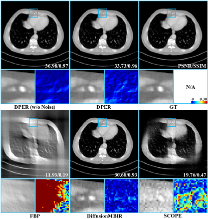
Figure 10: Qualitative and quantitative results of different methods to compare the measurement with the noise level of SNR $\approx$ 34 dB and without Noise on one test sample (#18) of the AAPM dataset for the LACT task of [0, 90]° scanning range.

Fig. 10 and Table 4 display the quantitative and qualitative results of the impact of different noise levels on our framework and other baselines for observing the robustness. There are some observations: 1) The results indicate that noise affects the model’s performance as it leads to a more ill-posed LACT inverse imaging problem. It is evident that as the noise level increases, the performance of all models deteriorates. However, the reduction ratio of self-supervised models shows better results than Prior-based methods, which is expected (The effect of diffusion prior is limited by noise measurement). 2) Compared to the FBP result with noise, the DPER result is significantly cleaner and maintains the data fidelity, which represents that the DPER framework can adapt to a single instance with different noise levels. 3) Compared to the SOTA DiffusionMBIR, our framework still maintains almost +2dB PSNR and +0.03 SSIM proportion of lead in all noise settings.

To summarize, the performance of all the methods is limited by noise in the measurement domain and our DPER can still preserve the best performance in all cases.

Table 4: Quantitative results (PSNR / SSIM) of different methods on the AAPM dataset test samples for LACT task of [0,90]° scanning range with three levels of noise (SNR = 32 dB, 37dB, 43 dB). The Best performances are highlighted in bold.

Method	32 dB	37 dB	43 dB
FBP	11.43 / 0.2018	11.47 0.2366	11.51 / 0.2974
SCOPE[20]	22.75 / 0.6829	23.08 0.7409	23.32 / 0.8124
DiffusionMBIR[35]	31.88 / 0.9234	33.07 0.9390	34.15 / 0.9503
DPER (Ours)	33.36 / 0.9459	34.52 0.9602	36.41 / 0.9685

5 Conclusion

This paper proposes DPER, an unsupervised DL model for highly ill-posed LACT and ultra-SVCT tasks. The proposed DPER follows the HQS framework to decompose the classical CT inverse problem into a data fidelity sub-problem and a distribution prior sub-problem. Then, the two sub-problems are respectively addressed by INR and a pre-trained diffusion model. The INR guarantees data consistency with incomplete CT measurements benefiting from the integration of the CT physical forward model, while the diffusion model provides a generative image prior effectively constraining the solution space. The empirical studies on two datasets reveal that the proposed DPER excels both quantitatively and qualitatively, establishing itself as the state-of-the-art performer on in-domain and out-of-domain datasets for the LACT problem, while for the ultra-SVCT problem, it demonstrates performance that is on par with other SOTA methods.

References

- [1] G. Wang, H. Yu, and B. De Man, “An outlook on x-ray ct research and development,” Medical physics, vol. 35, no. 3, pp. 1051–1064, 2008.
- [2] M. Katsura, I. Matsuda, M. Akahane, J. Sato, H. Akai, K. Yasaka, A. Kunimatsu, and K. Ohtomo, “Model-based iterative reconstruction technique for radiation dose reduction in chest ct: comparison with the adaptive statistical iterative reconstruction technique,” European radiology, vol. 22, pp. 1613–1623, 2012.
- [3] L. Liu, “Model-based iterative reconstruction: a promising algorithm for today’s computed tomography imaging,” Journal of Medical imaging and Radiation sciences, vol. 45, no. 2, pp. 131–136, 2014.
- [4] A. H. Andersen and A. C. Kak, “Simultaneous algebraic reconstruction technique (sart): a superior implementation of the art algorithm,” Ultrasonic imaging, vol. 6, no. 1, pp. 81–94, 1984.
- [5] R. Gordon, R. Bender, and G. T. Herman, “Algebraic reconstruction techniques (art) for three-dimensional electron microscopy and x-ray photography,” Journal of theoretical Biology, vol. 29, no. 3, pp. 471–481, 1970.
- [6] Y. Liu, J. Ma, Y. Fan, and Z. Liang, “Adaptive-weighted total variation minimization for sparse data toward low-dose x-ray computed tomography image reconstruction,” Physics in Medicine & Biology, vol. 57, no. 23, p. 7923, 2012.
- [7] Z. Chen, X. Jin, L. Li, and G. Wang, “A limited-angle ct reconstruction method based on anisotropic tv minimization,” Physics in Medicine & Biology, vol. 58, no. 7, p. 2119, 2013.
- [8] Y.-L. Sun and J.-X. Tao, “Image reconstruction from few views by l0-norm optimization,” Chinese Physics B, vol. 23, no. 7, p. 078703, 2014.
- [9] M. Xu, D. Hu, F. Luo, F. Liu, S. Wang, and W. Wu, “Limited-angle x-ray ct reconstruction using image gradient l0-norm with dictionary learning,” IEEE Transactions on Radiation and Plasma Medical Sciences, vol. 5, no. 1, pp. 78–87, 2020.
- [10] G. Wang, J. C. Ye, and B. De Man, “Deep learning for tomographic image reconstruction,” Nature Machine Intelligence, vol. 2, no. 12, pp. 737–748, 2020.
- [11] K. H. Jin, M. T. McCann, E. Froustey, and M. Unser, “Deep convolutional neural network for inverse problems in imaging,” IEEE transactions on image processing, vol. 26, no. 9, pp. 4509–4522, 2017.
- [12] Y. Han and J. C. Ye, “Framing u-net via deep convolutional framelets: Application to sparse-view ct,” IEEE transactions on medical imaging, vol. 37, no. 6, pp. 1418–1429, 2018.
- [13] Z. Zhang, X. Liang, X. Dong, Y. Xie, and G. Cao, “A sparse-view ct reconstruction method based on combination of densenet and deconvolution,” IEEE transactions on medical imaging, vol. 37, no. 6, pp. 1407–1417, 2018.
- [14] H. Lee, J. Lee, H. Kim, B. Cho, and S. Cho, “Deep-neural-network-based sinogram synthesis for sparse-view ct image reconstruction,” IEEE Transactions on Radiation and Plasma Medical Sciences, vol. 3, no. 2, pp. 109–119, 2018.
- [15] Y. Li, K. Li, C. Zhang, J. Montoya, and G.-H. Chen, “Learning to reconstruct computed tomography images directly from sinogram data under a variety of data acquisition conditions,” IEEE transactions on medical imaging, vol. 38, no. 10, pp. 2469–2481, 2019.
- [16] Y. Huang, A. Preuhs, G. Lauritsch, M. Manhart, X. Huang, and A. Maier, “Data consistent artifact reduction for limited angle tomography with deep learning prior,” in International workshop on machine learning for medical image reconstruction. Springer, 2019, pp. 101–112.
- [17] B. Zhou, S. K. Zhou, J. S. Duncan, and C. Liu, “Limited view tomographic reconstruction using a cascaded residual dense spatial-channel attention network with projection data fidelity layer,” IEEE transactions on medical imaging, vol. 40, no. 7, pp. 1792–1804, 2021.
- [18] H. Zhang, B. Liu, H. Yu, and B. Dong, “Metainv-net: Meta inversion network for sparse view ct image reconstruction,” IEEE Transactions on Medical Imaging, vol. 40, no. 2, pp. 621–634, 2020.
- [19] D. Hu, Y. Zhang, J. Liu, S. Luo, and Y. Chen, “Dior: Deep iterative optimization-based residual-learning for limited-angle ct reconstruction,” IEEE Transactions on Medical Imaging, vol. 41, no. 7, pp. 1778–1790, 2022.
- [20] Q. Wu, R. Feng, H. Wei, J. Yu, and Y. Zhang, “Self-supervised coordinate projection network for sparse-view computed tomography,” IEEE Transactions on Computational Imaging, vol. 9, pp. 517–529, 2023.
- [21] Q. Wu, X. Li, H. Wei, J. Yu, and Y. Zhang, “Joint rigid motion correction and sparse-view ct via self-calibrating neural field,” in 2023 IEEE 20th International Symposium on Biomedical Imaging (ISBI), 2023, pp. 1–5.
- [22] D. Rückert, Y. Wang, R. Li, R. Idoughi, and W. Heidrich, “Neat: Neural adaptive tomography,” ACM Transactions on Graphics (TOG), vol. 41, no. 4, pp. 1–13, 2022.
- [23] R. Zha, Y. Zhang, and H. Li, “Naf: neural attenuation fields for sparse-view cbct reconstruction,” in Medical Image Computing and Computer Assisted Intervention–MICCAI 2022: 25th International Conference, Singapore, September 18–22, 2022, Proceedings, Part VI. Springer, 2022, pp. 442–452.
- [24] G. Zang, R. Idoughi, R. Li, P. Wonka, and W. Heidrich, “Intratomo: self-supervised learning-based tomography via sinogram synthesis and prediction,” in Proceedings of the IEEE/CVF International Conference on Computer Vision, 2021, pp. 1960–1970.
- [25] Y. Sun, J. Liu, M. Xie, B. Wohlberg, and U. S. Kamilov, “Coil: Coordinate-based internal learning for tomographic imaging,” IEEE Transactions on Computational Imaging, vol. 7, pp. 1400–1412, 2021.
- [26] A. W. Reed, H. Kim, R. Anirudh, K. A. Mohan, K. Champley, J. Kang, and S. Jayasuriya, “Dynamic ct reconstruction from limited views with implicit neural representations and parametric motion fields,” in Proceedings of the IEEE/CVF International Conference on Computer Vision, 2021, pp. 2258–2268.
- [27] L. Shen, J. Pauly, and L. Xing, “Nerp: implicit neural representation learning with prior embedding for sparsely sampled image reconstruction,” IEEE Transactions on Neural Networks and Learning Systems, 2022.
- [28] D. Ulyanov, A. Vedaldi, and V. Lempitsky, “Deep image prior,” in Proceedings of the IEEE Conference on Computer Vision and Pattern Recognition (CVPR), June 2018.
- [29] J. Yoo, K. H. Jin, H. Gupta, J. Yerly, M. Stuber, and M. Unser, “Time-dependent deep image prior for dynamic mri,” IEEE Transactions on Medical Imaging, vol. 40, no. 12, pp. 3337–3348, 2021.
- [30] K. Gong, C. Catana, J. Qi, and Q. Li, “Pet image reconstruction using deep image prior,” IEEE transactions on medical imaging, vol. 38, no. 7, pp. 1655–1665, 2018.
- [31] D. O. Baguer, J. Leuschner, and M. Schmidt, “Computed tomography reconstruction using deep image prior and learned reconstruction methods,” Inverse Problems, vol. 36, no. 9, p. 094004, 2020.
- [32] N. Rahaman, A. Baratin, D. Arpit, F. Draxler, M. Lin, F. Hamprecht, Y. Bengio, and A. Courville, “On the spectral bias of neural networks,” in International Conference on Machine Learning. PMLR, 2019, pp. 5301–5310.
- [33] Y. Song, L. Shen, L. Xing, and S. Ermon, “Solving inverse problems in medical imaging with score-based generative models,” in International Conference on Learning Representations, 2021.
- [34] H. Chung, B. Sim, D. Ryu, and J. C. Ye, “Improving diffusion models for inverse problems using manifold constraints,” Advances in Neural Information Processing Systems, vol. 35, pp. 25 683–25 696, 2022.
- [35] H. Chung, D. Ryu, M. T. McCann, M. L. Klasky, and J. C. Ye, “Solving 3d inverse problems using pre-trained 2d diffusion models,” in Proceedings of the IEEE/CVF Conference on Computer Vision and Pattern Recognition, 2023, pp. 22 542–22 551.
- [36] H. Chung, B. Sim, and J. C. Ye, “Come-closer-diffuse-faster: Accelerating conditional diffusion models for inverse problems through stochastic contraction,” in Proceedings of the IEEE/CVF Conference on Computer Vision and Pattern Recognition, 2022, pp. 12 413–12 422.
- [37] C. Peng, P. Guo, S. K. Zhou, V. M. Patel, and R. Chellappa, “Towards performant and reliable undersampled mr reconstruction via diffusion model sampling,” in International Conference on Medical Image Computing and Computer-Assisted Intervention. Springer, 2022, pp. 623–633.
- [38] L. I. Rudin, S. Osher, and E. Fatemi, “Nonlinear total variation based noise removal algorithms,” Physica D: nonlinear phenomena, vol. 60, no. 1-4, pp. 259–268, 1992.
- [39] M. Tancik, P. Srinivasan, B. Mildenhall, S. Fridovich-Keil, N. Raghavan, U. Singhal, R. Ramamoorthi, J. Barron, and R. Ng, “Fourier features let networks learn high frequency functions in low dimensional domains,” Advances in Neural Information Processing Systems, vol. 33, pp. 7537–7547, 2020.
- [40] T. Müller, A. Evans, C. Schied, and A. Keller, “Instant neural graphics primitives with a multiresolution hash encoding,” ACM Transactions on Graphics (ToG), vol. 41, no. 4, pp. 1–15, 2022.
- [41] D. Geman and C. Yang, “Nonlinear image recovery with half-quadratic regularization,” IEEE transactions on Image Processing, vol. 4, no. 7, pp. 932–946, 1995.
- [42] Y. Zhu, K. Zhang, J. Liang, J. Cao, B. Wen, R. Timofte, and L. Van Gool, “Denoising diffusion models for plug-and-play image restoration,” in Proceedings of the IEEE/CVF Conference on Computer Vision and Pattern Recognition, 2023, pp. 1219–1229.
- [43] H. E. Robbins, “An empirical bayes approach to statistics,” in Breakthroughs in Statistics: Foundations and basic theory. Springer, 1992, pp. 388–394.
- [44] Y. Song, J. Sohl-Dickstein, D. P. Kingma, A. Kumar, S. Ermon, and B. Poole, “Score-based generative modeling through stochastic differential equations,” arXiv preprint arXiv:2011.13456, 2020.
- [45] B. Kawar, M. Elad, S. Ermon, and J. Song, “Denoising diffusion restoration models,” Advances in Neural Information Processing Systems, vol. 35, pp. 23 593–23 606, 2022.
- [46] H. Chung, J. Kim, M. T. Mccann, M. L. Klasky, and J. C. Ye, “Diffusion posterior sampling for general noisy inverse problems,” in The Eleventh International Conference on Learning Representations, 2022.
- [47] Y. Wang, J. Yu, and J. Zhang, “Zero-shot image restoration using denoising diffusion null-space model,” in The Eleventh International Conference on Learning Representations, 2022.
- [48] C. H. McCollough, A. C. Bartley, R. E. Carter, B. Chen, T. A. Drees, P. Edwards, D. R. Holmes III, A. E. Huang, F. Khan, S. Leng et al., “Low-dose ct for the detection and classification of metastatic liver lesions: results of the 2016 low dose ct grand challenge,” Medical physics, vol. 44, no. 10, pp. e339–e352, 2017.
- [49] A. C. Kak and M. Slaney, Principles of computerized tomographic imaging. SIAM, 2001.
- [50] S. G. Armato III, G. McLennan, L. Bidaut, M. F. McNitt-Gray, C. R. Meyer, A. P. Reeves, B. Zhao, D. R. Aberle, C. I. Henschke, E. A. Hoffman et al., “The lung image database consortium (lidc) and image database resource initiative (idri): a completed reference database of lung nodules on ct scans,” Medical physics, vol. 38, no. 2, pp. 915–931, 2011.
- [51] D. P. Kingma and J. Ba, “Adam: A method for stochastic optimization,” arXiv preprint arXiv:1412.6980, 2014.
- [52] N. Müller, Y. Siddiqui, L. Porzi, S. R. Bulo, P. Kontschieder, and M. Nießner, “Diffrf: Rendering-guided 3d radiance field diffusion,” in Proceedings of the IEEE/CVF Conference on Computer Vision and Pattern Recognition, 2023, pp. 4328–4338.
- [53] J. Gu, A. Trevithick, K.-E. Lin, J. M. Susskind, C. Theobalt, L. Liu, and R. Ramamoorthi, “Nerfdiff: Single-image view synthesis with nerf-guided distillation from 3d-aware diffusion,” in International Conference on Machine Learning. PMLR, 2023, pp. 11 808–11 826.