Low-Rank Online Dynamic Assortment with Dual Contextual Information

Abstract

As e-commerce expands, delivering real-time personalized recommendations from vast catalogs poses a critical challenge for retail platforms. Maximizing revenue requires careful consideration of both individual customer characteristics and available item features to optimize assortments over time. In this paper, we consider the dynamic assortment problem with dual contexts – user and item features. In high-dimensional scenarios, the quadratic growth of dimensions complicates computation and estimation. To tackle this challenge, we introduce a new low-rank dynamic assortment model to transform this problem into a manageable scale. Then we propose an efficient algorithm that estimates the intrinsic subspaces and utilizes the upper confidence bound approach to address the exploration-exploitation trade-off in online decision making. Theoretically, we establish a regret bound of $\tilde{O}((d_{1}+d_{2})r\sqrt{T})$, where $d_{1},d_{2}$ represent the dimensions of the user and item features respectively, $r$ is the rank of the parameter matrix, and $T$ denotes the time horizon. This bound represents a substantial improvement over prior literature, made possible by leveraging the low-rank structure. Extensive simulations and an application to the Expedia hotel recommendation dataset further demonstrate the advantages of our proposed method.

Keywords— Bandit algorithm, low-rankness, online decision making, regret analysis, reinforcement learning

1 Introduction

The assortment selection problem is a key challenge for retailers, who often face constraints on the number of items they can offer customers despite having a wide array of products. In the dynamic e-commerce environment, rich real-time information about customers and items drives the need for personalized algorithms adept at adapting to changing conditions. In online retail, the platform determines product recommendations by leveraging past assortment offerings and the users’ choices on their assortment offerings. Figure 1 illustrates the contextual dynamic assortment problem: At each time, a customer arrives with user features, the platform estimates user preferences on items based on historical data and current features, selects a subset from the item catalog to present to the current user and records user choices for improving future assortment selection.

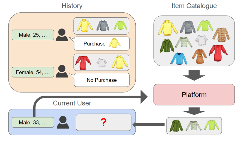
Figure 1: Illustration of the contextual dynamic assortment problem.

The primary objective of the platform is to maximize the total revenue over a time horizon $T$. It can adopt a ‘greedy strategy’ aimed at maximizing the revenue for each individual user by offering what is estimated as the best assortment at each time. However, due to the uncertainty of estimation, pure exploitation would lead to sub-optimal actions. To improve the accuracy of estimating these optimal assortments, the platform must delve into exploring user behaviors across various items. These two strategies, exploration for improving user preference estimation and exploitation for revenue maximization, often do not align in online decision making problems. Reinforcement learning, an area gaining increasing attention in statistics (Chakraborty and Murphy, , 2014; Zhao et al., , 2015; Shi et al., , 2018, 2023; Zhou et al., 2024b, ), provides valuable insights for navigating the delicate balance of the exploration-exploitation trade-off.

In recent years, a plethora of studies have utilized bandit and reinforcement learning algorithms (Lattimore and Szepesvári, , 2020) to address the dynamic assortment problem. Some research focuses on the non-contextual scenario (Chen and Wang, , 2018; Agrawal et al., , 2019), while others delve into the contextual setups (Chen et al., , 2020; Oh and Iyengar, , 2021; Goyal and Perivier, , 2022) under the multinomial logit (MNL) choice model (McFadden, , 1974) to characterize user behaviors. Advances in digital retail platform infrastructure have empowered these platforms with rich data on items and users, including demographics, search histories, and purchase records. By harnessing user features, the platform can tailor personalized assortments by looking back at the choice history of users with similar user contexts. Similarly, utilizing item features allows the platform to infer item preferences by analyzing the choice history of items sharing similar item contexts, even when the item has limited inclusion in assortment history. This motivates us to study the contextual dynamic assortment problem, specifically focusing on the incorporation of “dual contextual information” involving both items and users.

In contextual dynamic assortment, a common strategy for handling dual contexts is to stack the dual features as a joint feature vector and utilize its linear form (Sumida and Zhou, , 2023). Let $q_{t}\in\operatorname*{\mathbb{R}}^{d_{1}}$ be the vector representation of the feature of user $t$ and $p_{i}\in\operatorname*{\mathbb{R}}^{d_{2}}$ be a vector representation of the feature of item $i$. By stacking the dual features as $x_{it}=(1,p_{i}^{\top},q_{t}^{\top})^{\top}\in\operatorname*{\mathbb{R}}^{d_{1}+d_{2}+1}$, the utility of item $i$ for user $t$ is represented as $v_{it}=x_{it}^{\top}\phi$ with vector parameter $\phi\in\operatorname*{\mathbb{R}}^{d_{1}+d_{2}+1}$; see Figure 2.

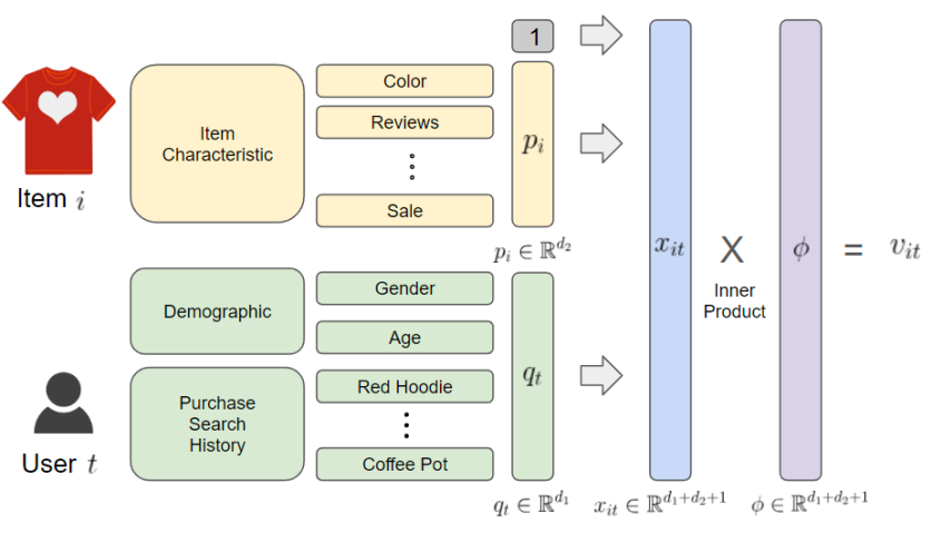
Figure 2: Stacked utility formulation of item and user features.

However, this approach fails to capture the interaction terms between the user feature and the item feature. Consider the effect of item price on the utility of an item to a user. The effect will be different across different users, some users might be sensitive to the price, while others may be not. Similarly, the red color of an item may have a positive effect on the utility if the user prefers red items, but will have a negative effect if the user dislikes red items. The additive nature of the stack formulation cannot capture this intrinsic interaction between the two sides of features.

Another approach involves utilizing the vectorization of the combined effects of the two features as a joint feature vector, followed by the application of existing contextual dynamic assortment selection methods (Agrawal et al., , 2019; Oh and Iyengar, , 2021). By including the intercept and taking the outer product of the two extended features, it accounts for the intercept, main effects, and user-item interaction effects simultaneously; see Figure 3. However, in high-dimensional settings, the dimension of the outer product is $(d_{1}+1)\times(d_{2}+1)$, which scales with the product of the dimensions of the dual features, making the estimation of the effects computationally challenging.

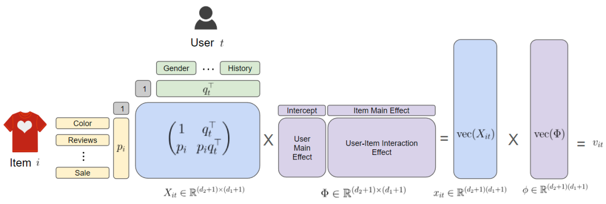
Figure 3: Vectorized utility formulation of interactions between user and item features.

In online retail, high-dimensional features can often be condensed into lower-dimensional latent factors. For instance, user traits like buying power can be inferred as a combination of income, education level, and past purchase behaviors. This buying power directly influences item utility, interacting with features such as price. Similarly, color preferences can be estimated from demographic data and previous red item purchases. Despite a user’s extensive purchase history spanning numerous items, its impact on red item utility can be simplified into a scalar value. Likewise, an item’s characteristics can be projected onto a reduced-dimensional latent space. Consequently, interaction effects between these dual contexts can be characterized by a smaller set of latent factors, as depicted in Figure 4.

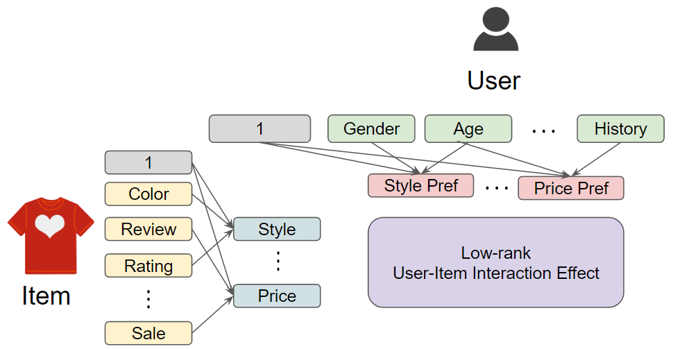
Figure 4: Illustration of low-rank user-item interaction effect.

By addressing the dual contextual problem within a low-rank structure, while retaining the impact of the features on the user preferences for items, we effectively reduce the dimension of the target parameter. This not only enhances computational efficiency but also reduces the cumulative estimation error across parameter components.

Inspired by this, in this paper we adopt the bilinear form $v=p^{\top}\Phi q$ with a low-rank matrix parameter $\Phi$ to represent utilities. This form offers flexibility, accommodating both stacking and vectorization approaches of incorporating dual features. The stack approach can be interpreted as the bilinear form with intercepts and a rank-2 parameter matrix while the vectorization approach can be interpreted as the scenario with full rank. Moreover, we can reduce the computational complexity by imposing a low-rank structure on $\Phi$, reducing the dimension of the parameter from $d_{1}d_{2}$ to $(d_{1}+d_{2})r$, where $r(\ll\min\{d_{1},d_{2}\})$ is the rank of the parameter matrix. Low-rank models have garnered growing interest in statistics (Jain et al., , 2013; Xia and Yuan, , 2021; Xia et al., , 2022; Ma et al., , 2024) with diverse scientific and business applications (Bell and Koren, , 2007; Koren et al., , 2009; Udell and Townsend, , 2019; Zhen and Wang, , 2024; Zhou et al., 2024a, ). Following this trend, our paper considers a new Low-rank Online Assortment with Dual-contexts (LOAD) problem.

To solve the LOAD problem, we propose an Explore-Low-rank-Subspace-then-Apply-UCB (ELSA-UCB) algorithm which consists of two main stages: subspace exploration and the application of Upper Confidence Bound (UCB). The major computational bottleneck arises from estimating the entire preference parameter matrix. To overcome this challenge, we project the features and parameters to a low-dimensional subspace. In the first stage, we leverage the inherent low-rank structure to estimate the low-dimensional subspace of the matrix parameter. To accomplish this, we explore the space by employing random assortments and then solve the rank-constrained likelihood maximization problem to estimate the subspace. Given the non-convex nature of the rank-constrained optimization problem, we adopt the alternating gradient descent algorithm based on the Burer-Monteiro formulation (Burer and Monteiro, , 2003; Zheng and Lafferty, , 2016; Chi et al., , 2019) to estimate the parameter matrix. Subsequently, we perform singular value decomposition (SVD) on the estimated matrix to derive the intrinsic subspace. Utilizing the estimated subspace, we rotate the features and parameters in accordance with the subspace, then truncate negligible terms to effectively reduce the problem’s dimensionality. In the second stage, we employ the UCB-based strategy on the reduced dimension based on careful construction of the confidence bounds in this space. UCB uses an “optimism in the face of uncertainty” idea that addresses the exploration-exploitation trade-off by selecting the best action based on the “optimistic reward”, the upper confidence bound of the estimated reward (Auer, , 2002; Lattimore and Szepesvári, , 2020). Contrary to the unbiased model in the original parameter space, the preference model within the reduced space, with respect to the estimated subspaces is inherently biased. To handle this, we introduce a novel tool that provides a confidence bound for the expected reward on the reduced space, by correcting this bias. Implementing the UCB-based policy in this reduced space reduces the parameter dimension from $d_{1}\times d_{2}$ to $r(d_{1}+d_{2})-r^{2}$. This reduction markedly improves computational efficiency, reduces estimation error, and enhances the algorithm performance.

To assess the theoretical performance of our proposed algorithm, we study the cumulative regrets of our policy. The regret is defined as the difference between the optimal reward from the oracle possessing complete knowledge of environmental parameters and the reward obtained from a given policy. In theory, we establish an $\tilde{O}((d_{1}+d_{2})r\sqrt{T})$ regret upper bound for our proposed ELSA-UCB policy (Theorem 1). Notably, in low-rank setups with $r\ll\min\{d_{1},d_{2}\}$, our regret bound is much improved from $\tilde{O}(d_{1}d_{2}\sqrt{T})$ regret bounds achieved by existing methods (Chen et al., , 2020; Oh and Iyengar, , 2021) that vectorize the outer product of the dual features.

The regret analysis for our policy presents several challenges. Firstly, in the dual-contextual environment, the distribution of joint features depends on the assortment selection, violating the i.i.d. feature assumption in existing dynamic assortment selection literature (Chen et al., , 2020; Oh and Iyengar, , 2021). To accommodate this, we impose minimal assumptions on the item features (Assumption 2) to ensure the identifiability of parameters. Secondly, the non-convex nature of the low-rank optimization problem precludes us from leveraging classical convex optimization theories. While Jun et al., (2019); Kang et al., (2022) studied generalized linear bandits with low-rank structure, their analysis tools are not applicable to our LOAD problem due to the unique combinatorial structure in the dynamic assortment selection. Thus, we establish novel estimation bounds specifically tailored for the rank-constrained optimization problem on assortment scenarios.

Finally, we present numerical results to demonstrate the effectiveness of our algorithm. Initially, we evaluate the ELSA-UCB policy’s performance on synthetic data, exploring various scenarios including changing ranks, feature dimensions, number of items, and assortment capacity. We compare cumulative regret over different time horizons with two variants of the UCB-MNL policy (Oh and Iyengar, , 2021): Stacked UCB-MNL and Vectorized UCB-MNL. Our analysis consistently shows that ELSA-UCB outperforms both methods across all scenarios, with the performance gap widening in scenarios with lower ranks and higher dimensions. Additionally, we conduct real data analysis on the Expedia dataset to optimize hotel recommendations. Our findings demonstrate that the parameter matrix exhibits a low-dimensional structure, and our method effectively leverages this to achieve improved performance, highlighting its practical usefulness.

1.1 Related Work

Our work is closely related to recent studies on contextual dynamic assortment selection and low-rank bandits. Additional relevant literature is provided in the Supplementary Materials.

1.1.1 Contextual Dynamic Assortment Selection

Inspired by the foundational work by Caro and Gallien, (2007), numerous studies have explored the dynamic assortment problem under the MNL bandit model. Various policies, including Explore-Then-Commit (Rusmevichientong et al., , 2010; Sauré and Zeevi, , 2013), Thompson Sampling (Agrawal et al., , 2017) and UCB (Agrawal et al., , 2019) have been proposed to address the balance between exploration and exploitation in the MNL bandit model. Other studies consider various scenarios such as robustness against outliers (Chen et al., , 2023), multi-stage choices (Xu and Wang, , 2023) or extension to different choice models (Aouad et al., , 2023). Contextual dynamic assortment considers various facets, including item-specific features (Wang et al., , 2019), time-varying item features (Chen et al., , 2020), user types (Kallus and Udell, , 2020), item features (Shao et al., , 2022), or features associated with user-item pairs (Oh and Iyengar, , 2021; Goyal and Perivier, , 2022). These features are utilized in modeling utilities for the MNL bandit model. However, while existing algorithms address single-context scenarios, focusing solely on users or items, they lack the capability to estimate interactions between dual contexts. Although algorithms designed for joint features on user-item pairs could be applied to the dual contextual setup by interpreting the vectorization of the outer product of dual features, this approach inevitably encounters large computational burdens and fails to capture the low-rank structure of the parameter matrix in our LOAD problem. Our proposed method aims to fill this gap.

1.1.2 Low-Rank Bandits

The dynamic environment involving high-dimensional covariates has also been a vibrant area of research. Based on a rich background of statistical tools for high dimensional problems (Wainwright, , 2019), numerous studies addressed the ‘curse of dimensionality’ in high-dimensional bandits. These studies often assume sparsity in the parameter vector and employ the LASSO-based approach (Abbasi-Yadkori et al., , 2012; Kim and Paik, , 2019) or presume the low-rank structure within the parameter matrix (Jun et al., , 2019; Kang et al., , 2022; Cai et al., , 2023; Zhou et al., 2024a, ). While certain studies have utilized the LASSO-based approach to address the sparse dynamic assortment problem (Wang et al., , 2019; Shao et al., , 2022), there has been comparatively less emphasis on leveraging the low-rank structure in the dynamic assortment. Recently, Cai et al., (2023) approached the dynamic assortment problem by modeling rewards as a bilinear form of action and context. However, they did not consider any user choice model and overlooked the inherent structure between assortment sets. Because of this, their algorithms and analysis tools are not applicable to our problem. To the best of our knowledge, our approach is the first one to incorporate the low-rank structure in the dynamic assortment selection with dual contexts.

2 Problem Formulation

In this section, we introduce the mathematical formulation of the LOAD problem. At time $t$, a user with feature vector $q_{t}\in\operatorname*{\mathbb{R}}^{d_{1}}$ arrives at the platform. Assume there are $N$ products, each with item feature vector $p_{i}\in\operatorname*{\mathbb{R}}^{d_{2}}$ for $i\in[N]=\{1,\ldots,N\}$. The platform offers an assortment $S_{t}$ of size at most $K$ from the catalog $[N]$. In other words, $S_{t}\subset[N]$ and $|S_{t}|\leq K$. When the user is provided with an assortment, the user either chooses one of the items in the assortment or chooses not to purchase at all. To quantify this user choice, let $y_{it}\in\{0,1\}$ represent whether user $t$ chooses item $i$, for $i\in[N]$ and $t\geq 1$. In addition, denote $y_{0t}=1$ as the indicator that user $t$ does not choose any item at all. Let $i_{t}\in S_{t}$ be the item that user $t$ chooses ($0$ if no purchase). Note that for at each user $t$, $y_{i_{t},t}=1$ and the remaining is $y_{jt}=0$ for $j\in S_{t}\cup\{0\}\backslash\{i_{t}\}$, i.e., $\sum_{i\in S_{t}\cup\{0\}}y_{it}=1$. Denote $\textbf{y}_{t}=(y_{1t},\ldots,y_{Nt})^{\top}\in\{0,1\}^{N}$ as the choice vector of user $t$.

In assortment selection, a widely adopted choice model is the multinomial logit (MNL) model (McFadden, , 1974; Rusmevichientong et al., , 2010; Agrawal et al., , 2019). Suppose the utility of item $i$ to user $t$ is given as a random variable $X_{it}=v_{it}+\epsilon_{it}$, where $v_{it}$ is the expected utility and $\epsilon_{it}$ is a mean-zero error term.Assume $v_{0t}=0$ for identifiability. The MNL model assumes that the probability of user $t$ choosing item $i$ is given as:

$$p_{t}(i):=\operatorname*{\mathbb{P}}(y_{it}=1)=\frac{\exp(v_{it})}{1+\sum_{j\in S_{t}}\exp(v_{jt})},\quad i\in S_{t},$$

and the probability of no purchase is given as $1/(1+\sum_{j\in S_{t}}\exp(v_{jt}))$. In this paper, we model the utility $v_{it}$ as a low-rank bilinear form of the dual contexts with

$$v_{it}=p_{i}^{\top}\Phi^{*}q_{t},$$

where $\Phi^{*}\in\operatorname*{\mathbb{R}}^{d_{2}\times d_{1}}$ is a rank-$r$ matrix, illustrated in Figure 4, with singular values $\sigma_{1}>\cdots\sigma_{r}>0$.

After the user’s purchasing decision under the MNL model, the platform earns revenue from the selected item (or zero if no purchase is made). Let $r_{i}$ denote the revenue that the platform achieves when item $i$ is sold. Given an assortment $S$, the revenue that the platform achieves from user $t$ is $\sum_{i\in S}r_{i}y_{it}$, and the expected revenue of the platform for user $t$ is:

$$R_{t}(S,\Phi^{*})=\operatorname*{\mathbb{E}}\left[\sum_{i\in S}r_{i}\cdot y_{it}\right]=\sum_{i\in S}r_{i}p_{t}(i|S,\Phi^{*}).$$

The platform aims to choose the personalized assortment for each user $t$ at time $t$ to maximize the cumulative expected revenue gained from all users. Note that the possible assortment set with constraint $K$, i.e., $\operatorname*{\mathcal{S}}=\{S\subset[N]:|S|\leq K\}$ is finite. Therefore, when $\Phi^{*}$ is known in hindsight, there exists an optimal assortment $S_{t}^{*}$ for user $t$ that maximizes the expected revenue since we can calculate the expected utility for every $S\in\operatorname*{\mathcal{S}}$. Denote the optimal assortment at time $t$ as:

$$S_{t}^{*}=\operatorname*{arg\,max}_{S\in\operatorname*{\mathcal{S}}}R_{t}(S,\Phi^{*}).$$

However, in practice, the true parameter $\Phi^{*}$ is not known to the platform. Instead, the platform chooses the assortment for each user $t$ based on some policy. To evaluate the performance of a policy, we define regret as the difference in expected revenue between the optimal assortment and the chosen assortment from the given policy. In other words, if we choose assortments $S_{t}$ for each user $t$, the total cumulative regret over time horizon $T$ is defined as

$${\operatorname*{\mathcal{R}}}_{T}=\operatorname*{\mathbb{E}}\left[\sum_{t=1}^{T}\left(R_{t}(S_{t}^{*},\Phi^{*})-R_{t}(S_{t},\Phi^{*})\right)\right].$$

Note that maximizing the cumulative revenue is equivalent to minimizing the cumulative regret. At time $t$, given the current user context $q_{t}$ and historical data, including past assortments $S_{1},S_{2},\ldots,S_{t-1}$ presented to users $1,2,\ldots,t-1$ with respective features $q_{1},q_{2},\ldots,q_{t-1}$, and the corresponding feedback $\textbf{y}_{1},\textbf{y}_{2},\ldots,\textbf{y}_{t-1}$, the platform needs to determine the assortment $S_{t}$ for the user $t$ so that the cumulative regret could be small.

3 Algorithm

In this section, we propose our Explore-Low-rank-Subspace-then-Apply-UCB (ELSA-UCB) method to address the LOAD problem defined in the previous section. The algorithm is mainly composed of two stages. The first stage is the exploration stage with random assortments which aims to estimate the low-dimensional subspace of the matrix parameter $\Phi^{*}$. Using the estimated subspace, we rotate the parameter and feature space and truncate the negligible dimensions. In the second stage, we use a UCB-based approach on the estimated subspace to select the assortment with the highest possible reward.

3.1 Estimation of Subspace

The first stage of the algorithm aims to acquire estimations of low-rank subspaces. Let $\Phi^{*}=U^{*}D^{*}(V^{*})^{\top}$ be the singular value decomposition of $\Phi^{*}$, where $U^{*}\in\operatorname*{\mathbb{R}}^{d_{2}\times d_{2}},V^{*}\in\operatorname*{\mathbb{R}}^{d_{1}\times d_{1}}$ are square orthonormal matrices and $D^{*}\in\operatorname*{\mathbb{R}}^{d_{2}\times d_{1}}$ is a diagonal matrix with singular values as its diagonal components. Let $u^{*}_{(j)}$ be the $j$-th column of $U^{*}$ and $v^{*}_{(j)}$ be the $j$-th column of $V^{*}$. Consider dual contexts $p\in\operatorname*{\mathbb{R}}^{d_{2}}$ and $q\in\operatorname*{\mathbb{R}}^{d_{1}}$. The bilinear form of $p$ and $q$ with respect to $\Phi^{*}$ can be rewritten as:

$$p^{\top}\Phi^{*}q=((U^{*})^{\top}p)^{\top}D^{*}((V^{*})^{\top}q)=\sum_{j=1}^{r}d_{j}p^{\prime}_{j}q^{\prime}_{j},$$

where $p^{\prime}_{j}=(u^{*}_{(j)})^{\top}p$ and $q^{\prime}_{j}=(v^{*}_{(j)})^{\top}q$ are rotations of $p$ and $q$ each with respect to orthonormal basis $U^{*}$ and $V^{*}$. Thus, the first $r$ columns of $U$ and $V$ each capture the $r$ latent features originating from dual contexts, which affect user preferences toward items. Consequently, by estimating the subspace of the matrix $\Phi^{*}$ via estimating $U^{*}$ and $V^{*}$, the platform effectively extracts the low-dimensional latent features, maintaining the representational capability of the original features.

For estimation of the subspace, we start with random assortments offered to the first $T_{0}$ users to achieve an initial estimate of $\Phi^{*}$. Consider the rank-constrained likelihood maximization problem:

$$\min_{\Phi\in\operatorname*{\mathbb{R}}^{d_{2}\times d_{1}},\ \text{rank}(\Phi)\leq r}{\operatorname*{\mathcal{L}}}_{n}(\Phi),$$ (1)

where $\operatorname*{\mathcal{L}}_{n}(\Phi)$ is the negative log-likelihood of the MNL choice model with $n$ samples:

$${\operatorname*{\mathcal{L}}}_{n}(\Phi)=-\frac{1}{n}\sum_{t=1}^{n}\left[\sum_{i\in S_{t}}y_{it}p_{i}^{\top}\Phi q_{t}-\log\left(1+\sum_{j\in S_{t}}\exp(p_{j}^{\top}\Phi q_{t})\right)\right].$$

To solve this rank-constrained optimization, we use the Burer-Monteiro formulation (Burer and Monteiro, , 2003) to optimize over $U\in\operatorname*{\mathbb{R}}^{d_{2}\times r}$ and $V\in\operatorname*{\mathbb{R}}^{d_{1}\times r}$, where $\Phi=UV^{\top}$. We add a regularization term to enforce identifiability (Zheng and Lafferty, , 2016). This leads to our final optimization problem:

$$\min_{U\in\operatorname*{\mathbb{R}}^{d_{2}\times r},\ V\in\operatorname*{\mathbb{R}}^{d_{1}\times r}}\left(\tilde{\operatorname*{\mathcal{L}}}_{n}(U,V):={\operatorname*{\mathcal{L}}}_{n}(UV^{\top})+\frac{1}{8}\|U^{\top}U-V^{\top}V\|_{F}^{2}\right).$$ (2)

This non-convex optimization can be solved effectively via an alternating factored gradient descent (FGD). FGD simply applies gradient descent on each factor,

$$U\leftarrow U-\eta\cdot\nabla_{U}\tilde{\operatorname*{\mathcal{L}}}_{n}(U,V),\quad V\leftarrow V-\eta\cdot\nabla_{V}\tilde{\operatorname*{\mathcal{L}}}_{n}(U,V),$$

where $\eta$ is the learning rate, $\nabla_{U},\nabla_{V}$ are gradients with respect to each component when other parameters are fixed. Applying these gradient descent steps alternatively, the estimated parameters are known to converge to the true parameters given conditions on the initial estimate (Zheng and Lafferty, , 2016; Zhang et al., , 2023). Details of FGD are given in Algorithm 1.

Algorithm 1 FGD - Factored Gradient Descent

1:Gradients of the loss function $\nabla_{U}\operatorname*{\mathcal{L}}$ and $\nabla_{V}\operatorname*{\mathcal{L}}$, initial estimate $\Phi_{0}$ and step size $\eta$.

2:SVD $\Phi_{0}=U_{0}D_{0}V_{0}^{\top}$ and initialize $U^{(0)}=U_{0}D_{0}^{1/2}$ and $V^{(0)}=V_{0}D_{0}^{1/2}$.

3:for $k=1,\ldots$, do

4:    Update $U^{(k+1)}=U^{(k)}-\eta\nabla_{U}{\operatorname*{\mathcal{L}}}|_{U=U^{(k)},V=V^{(k)}}$.

5:    Update $V^{(k+1)}=V^{(k)}-\eta\nabla_{V}{\operatorname*{\mathcal{L}}}|_{U=U^{(k+1)},V=V^{(k)}}$.

6:    Repeat until objective function converges.

7:end for

return $\hat{\Phi}=U^{(k)}(V^{(k)})^{\top}$.

For the initialization of FGD, we use the unconstrained maximum likelihood estimator (MLE) of $\Phi^{*}$. As the likelihood function is convex, we can apply a convex optimization algorithm such as the gradient-based algorithm or L-BFGS (Liu and Nocedal, , 1989) to calculate the initialization.

With the estimate $\hat{\Phi}$ from Algorithm 1, we obtain the estimated subspaces $\hat{U}$ and $\hat{V}$ via SVD, $\hat{\Phi}=\hat{U}\hat{D}\hat{V}^{\top}$. Next, we rotate the original subspace with respect to the estimated subspace. We partition $U^{*},V^{*},\hat{U},\hat{V}$ into $(U^{*}_{1},U_{2}^{*}),(V_{1}^{*},V_{2}^{*}),(\hat{U}_{1},\hat{U}_{2}),(\hat{V}_{1},\hat{V}_{2})$, where $(\cdot)_{1}$ denotes the first $r$ columns and $(\cdot)_{2}$ denotes the remaining columns of a matrix. Define:

$$\Theta^{*} :=\hat{U}^{\top}\Phi^{*}\hat{V}=(\hat{U}_{1},\hat{U}_{2})^{\top}U_{1}^{*}D_{11}(V_{1}^{*})^{\top}(\hat{V}_{1},\hat{V}_{2})$$

$$=\begin{pmatrix}(\hat{U}_{1}^{\top}U_{1}^{*})D_{11}^{*}(\hat{V}_{1}^{\top}V_{1}^{*})^{\top}&(\hat{U}_{1}^{\top}U_{1}^{*})D_{11}^{*}(\hat{V}_{2}^{\top}V_{1}^{*})^{\top}\\ (\hat{U}_{2}^{\top}U_{1}^{*})D_{11}^{*}(\hat{V}_{1}^{\top}V_{1}^{*})^{\top}&(\hat{U}_{2}^{\top}U_{1}^{*})D_{11}^{*}(\hat{V}_{2}^{\top}V_{1}^{*})^{\top}\end{pmatrix}.$$

We adopt the “subtraction method” prevalent in the low-rank matrix bandit (Kveton et al., , 2017; Jun et al., , 2019; Kang et al., , 2022). Note that $\hat{U}_{2}^{\top}U_{1}^{*}$ and $\hat{V}_{2}^{\top}V_{1}^{*}$ are expected to be small, assuming that $\hat{U},\hat{V}$ are good estimations of $U^{*},V^{*}$. Thus its product $(\hat{U}_{2}^{\top}U_{1}^{*})(\hat{V}_{2}^{\top}V_{1}^{*})^{\top}$ is expected to be negligible. To utilize this structure, we introduce the notation of “truncation-vectorization” of matrices. Consider $\Theta\in\operatorname*{\mathbb{R}}^{d_{2}\times d_{1}}$ with block-sub-matrices $\Theta_{11}\in\operatorname*{\mathbb{R}}^{r\times r}$, $\Theta_{12}\in\operatorname*{\mathbb{R}}^{r\times(d_{1}-r)}$, $\Theta_{21}\in\operatorname*{\mathbb{R}}^{(d_{2}-r)\times r}$, $\Theta_{22}\in\operatorname*{\mathbb{R}}^{(d_{2}-r)\times(d_{1}-r)}$. Define “truncation-vectorization” of $\Theta$ as

$$\theta_{rtv}:=(\operatorname*{\textup{vec}}(\Theta_{11})^{\top},\operatorname*{\textup{vec}}(\Theta_{12})^{\top},\operatorname*{\textup{vec}}(\Theta_{21})^{\top})^{\top}\in{\operatorname*{\mathbb{R}}}^{(d_{1}+d_{2})r-r^{2}},$$ (3)

where “$rtv$” is an abbreviation of “rotation-truncation-vectorization” to represent that the original matrix $\Phi^{*}$ has been rotated with respect to $\hat{U}$ and $\hat{V}$, then truncated and vectorized.

Note that $\Theta^{*}_{22}=(\hat{U}_{2}^{\top}U_{1}^{*})D_{11}^{*}(\hat{V}_{2}^{\top}V_{1}^{*})^{\top}$ is expected to be negligible, so we only need to focus on the estimation of $\theta^{*}_{rtv}$, the truncation-vectorization of $\Theta^{*}$. The computational advantage of this is that the dimension of the parameter is now reduced from $d_{2}d_{1}$ of $\Theta^{*}$ to $r(d_{1}+d_{2})-r^{2}$ of $\theta^{*}_{rtv}$. In the rotated space, the user utility of an item is expressed as

$$v_{it}=p_{i}^{\top}\Phi^{*}q_{t}=(\hat{U}^{\top}p_{i})^{\top}\Theta^{*}(\hat{V}^{\top}q_{t})=\langle(\hat{U}^{\top}p_{i})(\hat{V}^{\top}q_{t})^{\top},\Theta^{*}\rangle.$$

Denote $X_{it}=(\hat{U}^{\top}p_{i})(\hat{V}^{\top}q_{t})^{\top}$ and define the truncation-vectorization of $X_{it}$ as $x_{it,rtv}$. Then

$$v_{it}=\langle X_{it},\Theta^{*}\rangle=\langle x_{it,rtv},\theta_{rtv}\rangle+\langle(X_{it})_{22},\Theta^{*}_{22}\rangle\approx\langle x_{it,rtv},\theta_{rtv}\rangle,$$

as $\Theta^{*}_{22}\approx 0$. Hence we can represent our original dual features as $x_{it,rtv}$ and focus on the estimation of low-dimensional parameter $\theta_{rtv}$ for our dynamic assortment selection policy.

3.2 UCB-based Stage

The second stage of the algorithm employs the UCB approach on $\theta^{*}_{rtv}$. UCB algorithm, also known as “optimism in the face of uncertainty” (Lattimore and Szepesvári, , 2020), operates based on the principle that the decision-maker should select the assortment with the highest “optimistic reward”, or the upper confidence bound of the estimated reward. Even if an assortment has a low estimated expected reward, when it has a high upper confidence bound due to large uncertainty, the algorithm can still favor that assortment. This approach inherently strikes a balance between exploiting the estimated reward and exploring assortments with higher uncertainty. As the algorithm is encouraged to further explore assortments with greater uncertainty, the confidence bounds gradually tighten, converging towards the true expected reward.

To adopt the UCB approach, we formulate the optimistic utility of item $i$ to user $t$ as

$$z_{it}=x_{it,rtv}^{\top}\widehat{\theta}_{t,rtv}+\beta_{it}.$$ (4)

The first term $x_{it,rtv}^{\top}\widehat{\theta}_{t,rtv}$ is the estimate for utility of the item $i$ for user $t$, and the latter term $\beta_{it}$ quantifies the uncertainty of the utility. For $\beta_{it}$, it can be calculated as $\beta_{it}=\alpha_{t}\cdot\|x_{it,rtv}\|_{W_{t}^{-1}}$, where the selection of $\alpha_{t}$ is based on the confidence bound of $\widehat{\theta}_{t,rtv}$ established in Lemma 1 of Section 4 and $W_{t}=\sum_{s=1}^{t}\sum_{i\in S_{s}}x_{is,rtv}x_{is,rtv}^{\top}$. Then we choose the optimal assortment that maximizes the revenue under the optimistic utilities. In other words, we offer the assortment $S_{t}=\operatorname*{arg\,max}_{S\in\operatorname*{\mathcal{S}}}\tilde{R}_{t}(S)$, where

$$\tilde{R}_{t}(S):=\sum_{i\in S}r_{i}\cdot\frac{\exp(z_{it})}{1+\sum_{j\in S}\exp(z_{it})}.$$

After obtaining the optimistic utilities, this problem can be solved via the StaticMNL policy introduced for the static assortment problem (Rusmevichientong et al., , 2010).

During the construction of confidence bounds for the optimistic reward, the algorithm simultaneously updates the estimate $\widehat{\theta}_{t,rtv}$. Distinct from the rank-constrained MLE in the first stage, in the UCB-based stage we solve a new estimator for the updated parameter $\theta^{*}_{rtv}$. Since the parameter dimensionality has reduced from $d_{1}\times d_{2}$ in the first stage to $(d_{1}+d_{2})r-r^{2}$ in this UCB-stage, we can calculate the MLE directly on the reduced space to obtain $\widehat{\theta}_{n,rtv}=\operatorname*{arg\,min}\operatorname*{\mathcal{L}}_{n,rtv}(\theta_{rtv})$, where $\operatorname*{\mathcal{L}}_{n,rtv}$ is the negative log-likelihood in the reduced space with

$${\operatorname*{\mathcal{L}}}_{n,rtv}(\theta_{rtv})=\frac{1}{n}\sum_{t=1}^{n}\left[\sum_{i\in S_{t}}y_{it}x_{it,rtv}^{\top}\theta_{rtv}-\log\left(1+\sum_{j\in S_{t}}\exp(x_{it,rtv}^{\top}\theta_{rtv})\right)\right].$$ (5)

It is crucial to note that this optimization problem is simpler than the rank-constrained MLE in (1) or (2), since this optimization is unconstrained and many existing convex optimization techniques can be employed to solve (5).

Algorithm 2 ELSA-UCB - Explore Low-dimensional Subspace then Apply UCB

1:Assortment capacity $K$, rank of parameter matrix $r$, learning rate $\eta$, initial parameter estimate $\Phi_{0}$ and exploration length $T_{0}$.

2:Observe item feature vectors $p_{i}$, $i\in[N]$.

3:for $t=1,\ldots,T_{0}$, do

4:    Observe the current user feature vector $q_{t}$.

5:    Randomly select a size $K$ assortment $S_{t}\in\operatorname*{\mathcal{S}}$ and observe user choice $\mathbf{y}_{t}$.

6:end for

7:Estimate the low-rank matrix $\hat{\Phi}=\operatorname*{arg\,max}_{rk(\Phi)=r}{\operatorname*{\mathcal{L}}}_{n}(\Phi)$ using Algorithm 1.

8:Estimate the subspace using SVD $\hat{\Phi}=\hat{U}\hat{D}\hat{V}^{\top}$.

9:Initialize $\widehat{\theta}_{t,rtv}\in\operatorname*{\mathbb{R}}^{k}$ as the truncated vectorization of $\hat{D}$ as in (3).

10:Rotate the item features $p_{i}^{\prime}=\hat{U}^{\top}p_{i}$ for $i\in[N]$.

11:for $t=T_{0}+1,\ldots,T$, do

12:    Observe user feature vector $q_{t}$

13:    Rotate the user feature $q_{t}^{\prime}=\hat{V}^{\top}q_{t}$.

14:    Compute $x_{it,rtv}$, the truncated vectorization of $p_{i}^{\prime}(q_{t}^{\prime})^{\top}$ as in (3).

15:    Compute $z_{it}=x_{it,rtv}^{\top}\widehat{\theta}_{t,rtv}+\beta_{it}$ as in (4).

16:    Select $S_{t}=\operatorname*{arg\,max}_{S}\tilde{R}_{t}(S)$ via StaticMNL and observe choice $\mathbf{y}_{t}$.

17:    Update the MLE $\widehat{\theta}_{t,rtv}$ by solving (5).

18:end for

4 Theory

In this section, we first state and discuss the feasibility of the required assumptions (Section 4.1). Next, we derive the estimation error bound on our rank-constrained maximum likelihood estimation for the LOAD problem (Proposition 1), and use this result to establish a confidence bound on the parameter in the reduced space (Lemma 1). Finally we establish an upper bound on the regret of our ELSA-UCB policy (Theorem 1).

4.1 Assumptions

First, we impose conditions on the distribution of the feature vectors.

Assumption 1 (Distribution of user features).

Each user feature $q_{t}$ is i.i.d. from an unknown distribution, where $\|q_{t}\|_{2}\leq S_{q}$ for some constant $S_{q}$ and $\operatorname*{\mathbb{E}}[q_{t}q_{t}^{\top}]=\Sigma_{q}$ with positive definite $\Sigma_{q}$. Moreover, $\Sigma_{q}^{-1/2}q_{t}$ is $\sigma$-sub-Gaussian and its $\ell_{2}$ norm bounded by some constant $S_{v}$.

The boundness of feature vectors is common in contextual bandit and assortment problems (Li et al., , 2017; Oh and Iyengar, , 2021), and the invertibility of the second moment ensures that the distribution of user features is sufficient to estimate the related parameters. In addition, note that we only require i.i.d. condition on the user features, not on the joint user and item features as in existing dynamic assortment literature (Oh and Iyengar, , 2021; Chen et al., , 2020).

Assumption 2 (Design of item features).

The item features satisfy $\|p_{i}\|_{2}\leq S_{p}$ for some constant $S_{p}$ and assume $\Sigma_{p}:=\frac{1}{N}\sum_{i=1}^{N}p_{i}p_{i}^{\top}$ is positive definite.

We assume that item features are also bounded with an postive definite second moment. Note that the postive definite condition is needed to guarantee the identifiability of the matrix parameter $\Phi^{*}$, and can be verified in practice since $p_{i}$’s are given in advance. Next, we impose a standard assumption in contextual MNL problems (Oh and Iyengar, , 2021), which is a slight modification of the assumption on the link function in generalized linear contextual bandits (Li et al., , 2017).

Assumption 3.

There exists a constant $\kappa>0$ such that

$$\min_{\|\Phi-\Phi^{*}\|_{F}^{2}\leq 1}p_{t}(i|S,\Phi)p_{t}(0|S,\Phi)\geq\kappa,$$

for every $S\in\operatorname*{\mathcal{S}}$, $i\in S$ and $t\in[T]$, where $p_{t}(i|S,\Phi)$ is the probability of selecting item $i$ for user $t$ under the true parameter $\Phi$ and assortment $S$.

4.2 Main Results

We first establish an estimation error bound on our rank-constrained maximum likelihood estimation for the LOAD problem.

Proposition 1 (Accuracy of Low-Rank Estimation).

Suppose Assumptions 1, 2 and 3 hold. Further assume we have an initial estimate $\Phi_{0}\in\operatorname*{\mathbb{R}}^{d_{2}\times d_{1}}$ such that $\|\Phi_{0}-\Phi^{*}\|_{F}\leq c_{2}\sqrt{\sigma_{r}^{*}}$ for some constant $c_{2}$. Let $\hat{\Phi}$ be the rank-constrained estimator using Algorithm 1 with initial estimate $\Phi_{0}$. If the exploration length $T_{0}$ satisfies

$$T_{0}\geq 4\sigma^{2}(C_{1}\sqrt{d_{1}d_{2}}+C_{2}\sqrt{\log(1/\delta)})^{2}+\frac{2B}{\lambda_{\min}(\Sigma)K},$$

for some constant $C_{1},C_{2}$ and any $\delta\in(0,1)$, $B>0$, where $\Sigma=\Sigma_{q}\otimes\Sigma_{p}$, then

$$\|\hat{\Phi}-\Phi^{*}\|_{F}^{2}\leq\frac{288\sigma_{1}^{2}}{\sigma_{r}\kappa}\left(\frac{3}{4}+\frac{8T_{0}}{\kappa B}+\frac{2}{K\|\Sigma\|_{2}}\right)\frac{Kr\log(\frac{d_{1}+d_{2}}{\delta})}{B}S_{2}^{4}$$

with probability at least $1-\delta$, where $S_{2}=\max\{S_{p},S_{q}\}$ is a constant.

Remark 1 (Initial Estimate $\Phi_{0}$).

Note that we require the initialization error $\|\Phi_{0}-\Phi^{*}\|_{F}^{2}$ to be bounded. This assumption, often referred to as the ‘basin of attraction’ is a standard practice in the non-convex low-rank matrix estimation literature (Jain et al., , 2013; Chi et al., , 2019). It ensures that the iterative algorithm converges to the desired target. Such assumptions are valid in diverse situations, such as when offline data are available, or when the length of the exploration stage is large enough to provide a warm start for the gradient descent algorithm.

Note that the result holds for an arbitrary choice of $B>0$. Increasing $B$ and therefore increasing the length of exploration $T_{0}$ will naturally decrease the estimation error. In this case, accurate estimation of the subspace will lead to better exploitation. However, increasing $T_{0}$ will also increase the total cumulative regret. Hence the choice of $T_{0}$ shows the exploration-exploitation trade-off. In our method, we choose the optimal length of exploration $T_{0}=O(\sqrt{T})$ to minimize the cumulative regret. Finally, note that the rate is proportional to the rank $r$, which would have been scaling with $\min\{d_{1},d_{2}\}$ without the low-rank assumption. This illustrates how the low-rank assumption plays a crucial role in reducing the estimation error.

Next we first establish confidence bound on the parameter $\theta^{*}_{rtv}$.

Lemma 1 (Confidence bound on reduced space).

Suppose Assumptions 1, 2 and 3 hold. Further assume that $\|\Theta^{*}_{r+1:d_{2},r+1:d_{1}}\|_{F}^{2}\leq S_{\perp}$ for some constant $S_{\perp}$. Let $\widehat{\theta}_{n,rtv}$ be the maximum likelihood estimator of $\theta^{*}_{rtv}$ using observations from user $t=1,\ldots,n$ by minimizing (5). Then,

$$\|\widehat{\theta}_{n,rtv}-\theta^{*}_{rtv}\|_{W_{n}} \leq\frac{1}{\kappa}\left(\sigma\sqrt{2df\log\left(1+\frac{n}{df}\right)+4\log{n}}+S_{2}^{2}\cdot S_{\perp}\cdot\sqrt{nK}\right)=:\alpha_{n}$$

with probability at least $1-1/n^{2}$, where $W_{n}=\sum_{t=1}^{n}\sum_{i\in S_{t}}x_{it,rtv}x_{it,rtv}^{\top}$ and $df=(d_{1}+d_{2})r-r^{2}$ is the dimension of the reduced space.

With this definition of $\alpha_{n}$, we can calculate the optimistic utility defined in (4). Finally, we establish a non-asymptotic upper bound on the cumulative regret of our ELSA-UCB algorithm.

Theorem 1 (Regret Bound of ELSA-UCB).

Suppose assumptions of Proposition 1 hold. Define

$$T_{0} :=4\sigma^{2}(C_{1}\sqrt{d_{1}d_{2}}+C_{2}\sqrt{\log{T}})^{2}+\frac{2B}{\lambda_{\min}(\Sigma)K},$$

$$S_{\perp} :=\frac{288\sigma_{1}^{3}}{\sigma_{r}^{3}\cdot\kappa}\cdot\left(\frac{3}{4}+\frac{8T_{0}}{\kappa B}+\frac{2}{K\|\Sigma\|_{2}}\right)\frac{Kr\log(\frac{d_{1}+d_{2}}{\delta})}{B}S_{2}^{4},$$

$$\alpha_{n} :=\frac{1}{\kappa}\left(\sigma\sqrt{2df\log\left(1+\frac{n}{df}\right)+4\log{n}}+S_{2}^{2}\cdot S_{\perp}\cdot\sqrt{nK}\right),$$

for any $B>0$, where $df=(d_{1}+d_{2})r-r^{2}$ is the degree of freedom on the reduced space. Then applying Algorithm 2 with $T_{0}$ and $\alpha_{n}$, the cumulative regret of our ELSA-UCB policy satisfies

$${\operatorname*{\mathcal{R}}}_{T}\leq R_{\max}\left(T_{0}+3+2\alpha_{T}\sqrt{T\cdot 2\cdot df\log(T/df)}+2S_{2}^{2}S_{\perp}(T-T_{0})\right),$$

where $R_{\max}=\max_{i\in[N]}r_{i}$.

Theorem 1 provides a detailed regret bound of our policy. When applying our policy to e-commerce applications with a large number of users (large $T$), we can further simply this rate. With the choice $B=b\sqrt{T}$ for some constant $b$, we have $S_{\perp}=O(r/\sqrt{T})$ by definition and therefore $\operatorname*{\mathcal{R}}_{T}=\tilde{O}(r(d_{1}+d_{2})\sqrt{T})$, where $\tilde{O}(\cdot)$ ignores some logarithm term. For $d$-dimensional contextual assortment problem, Chen et al., (2020) established an $\Omega(d\sqrt{T}/K)$ lower bound on the cumulative regret. As the capacity $K$ is the maximum number of items that are displayed each time, we can interpret $K$ as a constant, and consequently, the lower bound becomes $\Omega(d\sqrt{T})$. When these results are applied by interpreting vectorization of the outer product of dual features as a single feature, the lower bound becomes $\Omega(d_{1}d_{2}\sqrt{T})$, without the low-rank assumption. Our algorithm significantly reduces the rate of regret to $\tilde{O}(df\cdot\sqrt{T})$ in the low-rank regime.

Establishing this regret bound possesses two main technical challenges. The first challenge involves incorporating the low-rank structure. To address this, we utilize results from the low-rank matrix estimation literature and adapt them to the LOAD problem. This enables us to establish an estimation bound on the estimated subspace. The second challenge arises from the inherent combinatorial structure of the assortment problem. To overcome this, we construct bound on the difference between the reward in the original problem and the transformed problem in the reduced space, which enables us to establish regret bounds for our algorithm.

4.3 Proof Sketch of Regret Bound

This section provides an outline of the three major steps in the proof of Theorem 1. Detailed proofs are presented in the Supplementary Materials. Step 1, as shown in Proposition 1, establishes a bound on the bias induced from rotation and truncation of the parameter matrix. Step 2 shows a bound on the difference between the optimistic utility $z_{it}$ defined as (4) and the true utility $v_{it}$ (Lemma 2). Finally, using this bound on the optimistic utility, Step 3 derives a bound on the regret of the $t$-th user, and the final result on the bound of cumulative regret (Theorem 1).

As our proposed algorithm ELSA-UCB truncates the lower right sub-block matrix of the rotated matrix, it is sufficient to establish a bound on the sub-block matrix.

Proposition 2 (Bounds for Subspace Estimation).

Suppose assumptions of Proposition 1 hold. Further assume the exploration length $T_{0}$ satisfies

$$T_{0}\geq 4\sigma^{2}(C_{1}\sqrt{d_{1}d_{2}}+C_{2}\sqrt{\log(1/\delta)})^{2}+\frac{2B}{\lambda_{\min}(\Sigma)K},$$

for some constants $C_{1}$, $C_{2}$ and any $\delta\in(0,1)$, $B>0$. Denote the SVD of the rank-constrained estimator as $\hat{U}\hat{D}\hat{V}^{\top}$. Then rotated true parameter $\Theta^{*}=\hat{U}^{\top}\Phi^{*}\hat{V}$ satisfies

$$\|\Theta^{*}_{r+1:d_{2},r+1:d_{1}}\|_{F}^{2}\leq\frac{288\sigma_{1}^{3}}{\sigma_{r}^{3}\cdot\kappa}\cdot\left(\frac{3}{4}+\frac{8T_{0}}{\kappa B}+\frac{2}{K\|\Sigma\|_{2}}\right)\frac{Kr\log(\frac{d_{1}+d_{2}}{\delta})}{B}S_{2}^{4}=:S_{\perp}$$ (6)

with probability at least $1-\delta$.

Proposition 2 allows us to control the gap $S_{\perp}$ between the reduced subspace and the original subspace by controlling $B$, which relates to the exploration length. Next, we establish a bound on the difference between the optimistic utility $z_{it}=x_{it,rtv}^{\top}\widehat{\theta}_{t,rtv}+\alpha_{t}\cdot\|x_{it,rtv}\|_{W_{t}^{-1}}$ and the true utility $v_{it}=\langle X_{it},\Theta^{*}\rangle$ using Proposition 2.

Lemma 2 (Bound on Optimistic Utility).

Let $z_{it}=x_{it,rtv}^{\top}\widehat{\theta}_{t,rtv}+\beta_{it}$. Then for every $i\in[N]$,

$$0\leq z_{it}-\langle X_{it},\Theta^{*}\rangle\leq 2\beta_{it}=2\alpha_{t}\|x_{it,rtv}\|_{W_{t}^{-1}}+2S_{2}^{2}\cdot S_{\perp}$$

with probability at least $1-t^{-2}$.

Note that $z_{it}$ is greater than the true utility $v_{it}=\langle X_{it},\Theta^{*}\rangle$ of item $i$ to user $t$ with probability at least $1-t^{-2}$. Let us denote $R(\{w_{i}\},S)$ as the expected revenue of offering assortment $S$ under the MNL model assuming utility $w_{i}$ for each item. Let $S_{t}^{*}$ be the optimal assortment with respect to the true revenue $v_{it}$ and $S_{t}$ be the optimal assortment with respect to the optimistic revenue $z_{it}$. Then from the definition we have the following bound for regret $r_{t}$ for user $t$:

$$r_{t}=R(\{v_{it}\},S_{t}^{*})-R(\{v_{it}\},S_{t})\leq R(\{z_{it}\},S_{t}^{*})-R(\{v_{it}\},S_{t})\leq R(\{z_{it}\},S_{t})-R(\{v_{it}\},S_{t}).$$ (7)

Moreover, we can bound the last term using the result from Oh and Iyengar, (2021) that establishes a bound on the difference of expected reward of an assortment given different utilities:

Lemma 3 (Lemma 5 of Oh and Iyengar, (2021)).

Let $u_{i},u_{i}^{\prime},i\in[N]$ be utilities and suppose $0\leq r_{i}\leq R$ for every item $i\in[N]$. Then $R(\{u_{i}\},S)-R(\{u_{i}^{\prime}\},S)\leq R\cdot\max_{i\in S}|u_{i}-u^{\prime}_{i}|$.

Combining (7), Lemmas 2 and 3, we have

$${\operatorname*{\mathcal{R}}}_{T} =\sum_{t=1}^{T_{0}}r_{t}+\sum_{t=T_{0}+1}^{T}r_{t}$$

$$\leq R_{\max}T_{0}+R_{\max}\left(\sum_{t=T_{0}+1}^{T}2\alpha_{t}\max_{i\in S_{t}}\|x_{it,rtv}\|_{W_{t}^{-1}}+2S_{2}^{2}S_{\perp}(T-T_{0})\right).$$

Lastly, presenting an upper bound on $\sum_{t=T_{0}+1}^{T}2\alpha_{t}\max_{i\in S_{t}}\|x_{it,rtv}\|_{W_{t}^{-1}}$, we obtain our final result Theorem 1. Proofs of the theoretical results are presented in the Supplementary Materials.

5 Numerical Studies

In this section, we evaluate the cumulative regret of our ELSA-UCB policy across varying scenarios, including different numbers of users, feature dimensions, ranks of parameter matrix, numbers of items and capacity of the assortment. We begin by examining it using synthetic data in Section 5.1 and subsequently validate its practicability in a real-world dataset in Section 5.2.

5.1 Simulation

To generate the parameter matrix $\Phi^{*}$, we first construct a diagonal matrix $D^{*}$ with $r$ non-zero components, each set to be 10. Next we multiply random orthonormal matrices $U^{*}\in\operatorname*{\mathbb{R}}^{d_{2}\times r}$ and $V^{*}\in\operatorname*{\mathbb{R}}^{d_{1}\times r}$ to generate a random rank-$r$ matrix $\Phi^{*}=U^{*}D^{*}(V^{*})^{\top}\in\operatorname*{\mathbb{R}}^{d_{2}\times d_{1}}$. For the user features, we generate $q_{t}\in\operatorname*{\mathbb{R}}^{d_{1}}$ for every $t\in[T]$ from the $d_{1}$-dimensional standard Gaussian distribution. Similarly, for item features, we generate $p_{i}\in\operatorname*{\mathbb{R}}^{d_{2}}$ from the $d_{2}$-dimensional standard Gaussian distribution for every $i\in[N]$. Note that the $N$ item features are fixed over the time horizon while user features are generated at each time step. The revenue is set as $r_{i}=1$ for every $i\in[N]$, following the setup in Oh and Iyengar, (2021). This accounts for scenarios where the goal is to maximize the sum of a binary outcome, aiming to maximize the total number of conversions, such as clicks or purchases in online retail.

Utilizing the generated parameters and features, we simulate user choices and the corresponding assortment selections following the policy. We compare the performance of our proposed ELSA-UCB against two versions of the UCB-MNL (Agrawal et al., , 2019; Oh and Iyengar, , 2021). As UCB-MNL considers features for each user-item pair as $x_{it}$, we consider two formulations of the joint features; “stacked” and “vectorized”.

• Stacked UCB-MNL: As shown in Figure 2, we stack the user features and the item features together including intercept as $x_{it}=(1,p_{i},q_{t})=(1,p_{i1},p_{i2},\ldots,p_{id_{2}},q_{t1},\ldots q_{td_{1}})\in{\operatorname*{\mathbb{R}}}^{d_{1}+d_{2}+1}$, which allows the linear formulation of the utilities to take into account the main effects of both features with parameter $\theta=(\alpha,\beta_{1},\ldots,\beta_{d_{2}},\gamma_{1},\ldots,\gamma_{d_{1}})\in\operatorname*{\mathbb{R}}^{d_{1}+d_{2}+1}$ :

  $$v_{it}=\theta^{\top}x_{it}=\alpha+\sum_{j=1}^{d_{2}}p_{ij}\beta_{j}+\sum_{k=1}^{d_{1}}q_{tk}\gamma_{k}.$$

• Vectorized UCB-MNL: As shown in Figure 3, we consider the vectorization of the outer product of the dual features with intercept, $p_{i}^{\prime}=(1,p_{i1},\ldots p_{id_{2}})$ and $q_{t}^{\prime}=(1,q_{t1},\ldots,q_{td_{1}})$:

  $$X_{it} =p_{i}^{\prime}\otimes q_{t}^{\prime}=\begin{pmatrix}1&q_{t1}&\ldots&q_{td_{1}}\\ p_{i1}&p_{i1}q_{t1}&\ldots&p_{i1}q_{td_{1}}\\ \vdots&\vdots&\ddots&\vdots\\ p_{id_{2}}&p_{id_{2}}q_{t1}&\ldots&p_{id_{2}}q_{td_{1}}\end{pmatrix}\in{\operatorname*{\mathbb{R}}}^{(d_{2}+1)\times(d_{1}+1)},$$

  $$x_{it} =\operatorname*{\textup{vec}}(X_{it})=(1,p_{i1},\ldots,p_{id_{2}}q_{td_{1}})\in{\operatorname*{\mathbb{R}}}^{(d_{2}+1)(d_{1}+1)},$$

  as the joint feature for the user-item pair. This takes into account for the main effects and the interaction terms of the dual features with parameter $\theta=(\alpha,\ldots,\delta_{11},\ldots,\delta_{d_{2}d_{1}})\in\operatorname*{\mathbb{R}}^{(d_{2}+1)(d_{1}+1)}$, which leads to the following formulation of utilities:

  $$v_{it}=\theta^{\top}x_{it}=\alpha+\sum_{j=1}^{d_{2}}p_{ij}\beta_{j}+\sum_{k=1}^{d_{1}}q_{tk}\gamma_{k}+\sum_{j=1}^{d_{2}}\sum_{k=1}^{d_{1}}\delta_{jk}p_{ij}q_{tk}.$$

Note that the stacked formulation can be viewed as a special case of the vectorized formulation, when there is no interaction. In this case, the parameter matrix contains non-zero elements only on the first row and the first column, which restricts the rank of the matrix to be at most $2$.

We apply our proposed ELSA-UCB policy and the two variations of UCB-MNL as baselines for comparison. We repeat the simulation 10 times and plot the median and the 10th/90th percentile of the cumulative regret for each $T\in\{500,1000,2000,5000,10000\}$ under different environments.

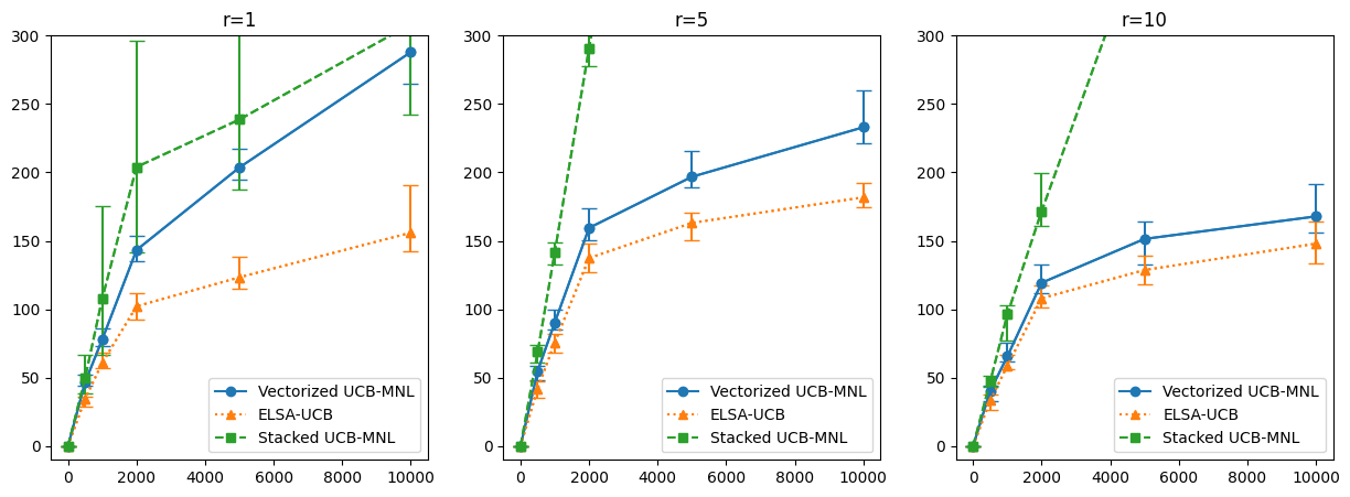
Figure 5: Cumulative regrets of our proposed ELSA-UCB algorithm compared with Stacked UCB-MNL and Vectorized UCB-MNL for different ranks $r\in\{1,5,10\}$.

For the first line of experiments, we fix $d_{1}=30,d_{2}=20,N=20,K=3$ and change the ranks $r\in\{1,5,10\}$ and number of users over $T=500,1000,2000,5000,10000$ and plot the corresponding cumulative regret in Figure 5. In higher ranks, the Stacked UCB-MNL produces larger cumulative regret, as it does not take consideration for the diverse interactions between the dual features. On the other hand, the Vectorized UCB-MNL has comparable performance when the rank is high. However, when the rank is low, the performance of Vectorized UCB-MNL is not satisfactory as it does not take account for the low-rank structure of the parameter matrix. Our ELSA-UCB policy universally outperforms both methods as it utilizes the low-rank structure and therefore efficiently estimate how the interactions between the dual features affect user preference of items.

Note that the cumulative regrets across different settings are not directly comparable. For example, in Figure 5, we observe a decrease in cumulative regrets for our method as the rank increases. This phenomenon occurs as we fix the scale for the singular values of $\Phi^{*}$, the intrinsic value $v_{it}$ increases, making it be easier to distinguish the optimal assortments. However, if we decrease the scale of the singular values as rank increases, the scale of the intrinsic value might remain the same, but the parameter estimation becomes challenging, potentially leading to performance degradation. Therefore, it would be fair to compare cumulative regret only within the same settings and compare the relative gap between different settings.

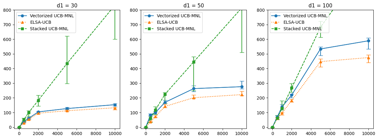
Figure 6: Plots of cumulative regret by $T$ for different dimensions.

In the next set of experiments, we fix $d_{2}=20,r=3,N=20,K=3$ while changing $d_{1}\in\{30,50,100\}$. The results are shown in Figure 6. The Stacked UCB-MNL shows poor performance across all dimensions. Moreover, we can observe that the gap between the cumulative regret of ELSA-UCB and Vectorized UCB-MNL widens as $d_{1}$ increases. This indicates that our algorithm is even preferable in environments with higher dimensional features. Furthermore, note that the scale of the regret increases as $d_{1}$ increases which aligns with the results of Theorem 1.

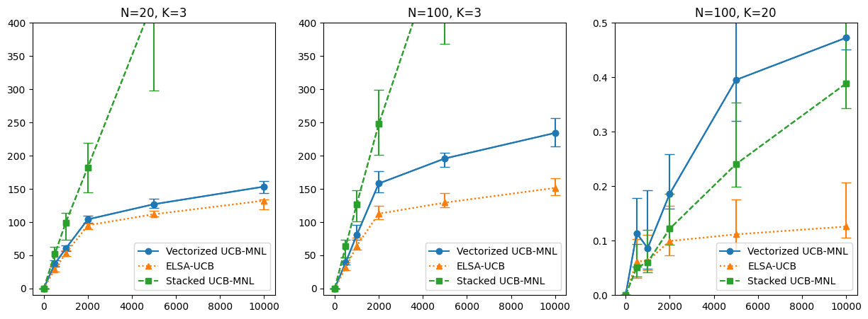
Figure 7: Plots of cumulative regret by $T$ for different numbers of items and capacity.

In the final set of experiments, we fix $d_{1}=30,d_{2}=20,r=3$ and change $(N,K)$ to be $\{(20,3),(100,3),(100,20)\}$. The results are illustrated in Figure 7. Note that as the assortment capacity $K$ increases, the gap between the optimal assortment and the near-optimal assortments decreases, resulting in smaller regrets. Overall, our proposed method outperforms both Stacked UCB-MNL and Vectorized UCB-MNL across all setups.

5.2 Real Data Application

In this section, we apply our algorithm to the “Expedia Hotel” dataset (Adam et al., , 2013) to evaluate its performance in real data.

5.2.1 Data Pre-processing

The dataset consists of 399,344 unique searches on 23,715 search destinations each accompanied by a recommendation of maximum 38 hotels from a pool of 136,886 unique properties. User responses are indicated by clicks or hotel room purchases. The dataset also includes features for each property-user pair, including hotel characteristics such as star ratings and location attractiveness, as well as user attributes such as average hotel star rating and prices from past booking history.

It is important to note that search queries constrain assortments to those within the search destination. We focus on data from the top destination with the highest search volume. Additionally, we filter out columns with missing over $90\%$ of searches. To address missing values in the remaining data for average star ratings and prices of each user from historical data, we employ a simple regression tree imputation. For hotel features, we compute the mean of feature values across searches. We discretize numerical features such as star ratings or review scores into categories to improve model fitting. After pre-processing, we have $T=4465$ unique searches encompassing $N=124$ different hotels, with $d_{2}=10$ hotel features and $d_{1}=18$ user features. The description of features is given in Table 1. We normalize each feature to have mean $0$ and variance $1$. As for the item features, we truncate the feature values between $[-3,3]$ to avoid the effect of outliers.

Item (Hotel) Features	Star rating (4 levels), Average review score (3 levels), Brand of property, Location score, Log historical price, Current price, Promotion
User (Search) Features	Length of stay (4 levels), Time until actual stay (4 levels), # of adults (3 levels), # of children (3 levels), # of rooms (2 levels), Inclusion of Saturday night, Website domain, User historical star rating (3 levels), User historical price (4 levels)

Table 1: Table of Item and User Features.

5.2.2 Analysis of the Expedia Dataset

To evaluate different dynamic assortment selection policies, we first estimate the ground truth parameter $\Phi^{*}$ using rank-constrained maximum likelihood estimation (1) on the full dataset. Note that as depicted in the left heatmap of Figure 8, the scale of the main effects (the first row and the first column) is larger than that of the interaction terms (the lower right matrix excluding first row and first column), implying that there is an inherent low-rank structure. Indeed, Akaike Information Criterion (AIC) (Bozdogan, , 1987) selects $r=8$ over a range of ranks.

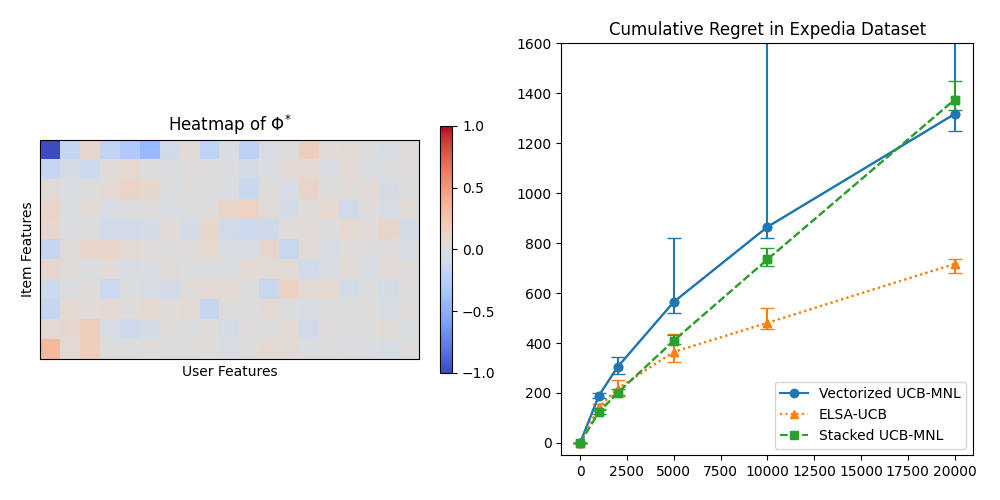
Figure 8: The left plot is the heatmap of ground truth parameter matrix $\Phi^{*}$. The right plot shows the cumulative regrets of different algorithms.

Following the approach in our simulation studies, we compare the cumulative regrets of our proposed ELSA-UCB policy with Stacked UCB-MNL and Vectorized UCB-MNL. We compare the performance of the algorithms for $T\in\{1000,2000,5000,10000,20000\}$. To evaluate the performance of the algorithm over an extended time horizon, we resample the users from the original data. As shown in the right plot of Figure 8, our proposed ELSA-UCB algorithm outperforms both Stacked UCB-MNL and Vectorized UCB-MNL in terms of cumulative regret. Notably, our advantage becomes more pronounced with an increasing time horizon. Moreover, we observe that Stacked UCB-MNL outperforms Vectorized UCB-MNL in shorter time horizons, while Vectorized UCB-MNL starts to outperform Stacked UCB-MNL in longer time horizons. This observation aligns with the finding illustrated in the left plot of Figure 8, where the main effect, depicted in the first row and first column of $\Phi^{*}$, significantly outweighs the interaction terms. In shorter time horizons, focusing on the main effect using Stacked UCB-MNL is advantageous compared to estimating every interaction term as in Vectorized UCB-MNL. However, in longer time horizons, Stacked UCB-MNL encounters estimation errors induced by completely ignoring the interaction terms. By avoiding unnecessary estimation of the whole parameter and focusing on learning in the reduced space, our proposed ELSA-UCB algorithm outperforms both Stacked UCB-MNL and Vectorized UCB-MNL.

6 Conclusion

In this paper, we explore the low-rank online dynamic assortment selection problem with dual contextual information. By incorporating the tools from low-rank matrix estimation into the construction of upper confidence bounds in MNL bandit problems, we propose a novel algorithm that addresses the dynamic assortment problem in high-dimensional settings. We provide a theoretical regret bound of our proposed algorithm which improves the rate in existing algorithms that do not consider the low-rank structure. We also provide numerical results on different settings to illustrate the performance gain of our proposed algorithm.

To conclude this paper, we outline some potential future research directions. While we have discussed dynamic assortment with varying items and user contexts, we have mainly focused on scenarios with fixed item catalogs. However, real-life applications often involve situations where the item catalog changes over time. Unlike the non-contextual environment which requires new inferences on new items, the contextual setup allows us to utilize contextual information of the new item to approximate their utility. Another topic of interest is the pricing strategies (Goyal and Perivier, , 2022; Luo et al., , 2024). Price affects both the utility of the item and the revenue gained from the item. The determination of optimal pricing introduces additional challenges for the platform in such scenarios. While there has been multiple research on dynamic pricing, it will be interesting to consider the dual contextual setup in dynamic pricing.

References

- Abbasi-Yadkori et al., (2012) Abbasi-Yadkori, Y., Pal, D., and Szepesvari, C. (2012). Online-to-confidence-set conversions and application to sparse stochastic bandits. In Artificial Intelligence and Statistics, pages 1–9. PMLR.
- Adam et al., (2013) Adam, Hamner, B., Friedman, D., and SSA_Expedia (2013). Personalize expedia hotel searches - ICDM 2013. Kaggle. https://kaggle.com/competitions/expedia-personalized-sort.
- Agrawal et al., (2017) Agrawal, S., Avadhanula, V., Goyal, V., and Zeevi, A. (2017). Thompson sampling for the MNL-bandit. In Conference on Learning Theory, pages 76–78. PMLR.
- Agrawal et al., (2019) Agrawal, S., Avadhanula, V., Goyal, V., and Zeevi, A. (2019). Mnl-bandit: A dynamic learning approach to assortment selection. Operations Research, 67(5):1453–1485.
- Aouad et al., (2023) Aouad, A., Feldman, J., and Segev, D. (2023). The exponomial choice model for assortment optimization: an alternative to the MNL model? Management Science, 69(5):2814–2832.
- Auer, (2002) Auer, P. (2002). Using confidence bounds for exploitation-exploration trade-offs. Journal of Machine Learning Research, 3(Nov):397–422.
- Bell and Koren, (2007) Bell, R. M. and Koren, Y. (2007). Lessons from the netflix prize challenge. Acm Sigkdd Explorations Newsletter, 9(2):75–79.
- Bozdogan, (1987) Bozdogan, H. (1987). Model selection and akaike’s information criterion (aic): The general theory and its analytical extensions. Psychometrika, 52(3):345–370.
- Burer and Monteiro, (2003) Burer, S. and Monteiro, R. D. (2003). A nonlinear programming algorithm for solving semidefinite programs via low-rank factorization. Mathematical Programming, 95(2):329–357.
- Cai et al., (2023) Cai, J., Chen, R., Wainwright, M. J., and Zhao, L. (2023). Doubly high-dimensional contextual bandits: An interpretable model for joint assortment-pricing. arXiv preprint arXiv:2309.08634.
- Caro and Gallien, (2007) Caro, F. and Gallien, J. (2007). Dynamic assortment with demand learning for seasonal consumer goods. Management Science, 53(2):276–292.
- Chakraborty and Murphy, (2014) Chakraborty, B. and Murphy, S. A. (2014). Dynamic treatment regimes. Annual Review of Statistics and Its Application, 1:447–464.
- Chen et al., (2023) Chen, X., Krishnamurthy, A., and Wang, Y. (2023). Robust dynamic assortment optimization in the presence of outlier customers. Operations Research.
- Chen and Wang, (2018) Chen, X. and Wang, Y. (2018). A note on a tight lower bound for capacitated mnl-bandit assortment selection models. Operations Research Letters, 46(5):534–537.
- Chen et al., (2020) Chen, X., Wang, Y., and Zhou, Y. (2020). Dynamic assortment optimization with changing contextual information. The Journal of Machine Learning Research, 21(1):8918–8961.
- Chi et al., (2019) Chi, Y., Lu, Y. M., and Chen, Y. (2019). Nonconvex optimization meets low-rank matrix factorization: An overview. IEEE Transactions on Signal Processing, 67(20):5239–5269.
- Goyal and Perivier, (2022) Goyal, V. and Perivier, N. (2022). Dynamic pricing and assortment under a contextual mnl demand. Advances in Neural Information Processing Systems, 35:3461–3474.
- Jain et al., (2013) Jain, P., Netrapalli, P., and Sanghavi, S. (2013). Low-rank matrix completion using alternating minimization. In Proceedings of the forty-fifth annual ACM symposium on Theory of Computing, pages 665–674.
- Jun et al., (2019) Jun, K.-S., Willett, R., Wright, S., and Nowak, R. (2019). Bilinear bandits with low-rank structure. In International Conference on Machine Learning, pages 3163–3172. PMLR.
- Kallus and Udell, (2020) Kallus, N. and Udell, M. (2020). Dynamic assortment personalization in high dimensions. Operations Research, 68(4):1020–1037.
- Kang et al., (2022) Kang, Y., Hsieh, C.-J., and Lee, T. C. M. (2022). Efficient frameworks for generalized low-rank matrix bandit problems. Advances in Neural Information Processing Systems, 35:19971–19983.
- Kim and Paik, (2019) Kim, G.-S. and Paik, M. C. (2019). Doubly-robust lasso bandit. Advances in Neural Information Processing Systems, 32:5877–5887.
- Koren et al., (2009) Koren, Y., Bell, R., and Volinsky, C. (2009). Matrix factorization techniques for recommender systems. Computer, 42(8):30–37.
- Kveton et al., (2017) Kveton, B., Szepesvári, C., Rao, A., Wen, Z., Abbasi-Yadkori, Y., and Muthukrishnan, S. (2017). Stochastic low-rank bandits. arXiv preprint arXiv:1712.04644.
- Lattimore and Szepesvári, (2020) Lattimore, T. and Szepesvári, C. (2020). Bandit algorithms. Cambridge University Press.
- Li et al., (2017) Li, L., Lu, Y., and Zhou, D. (2017). Provably optimal algorithms for generalized linear contextual bandits. In International Conference on Machine Learning, pages 2071–2080. PMLR.
- Liu and Nocedal, (1989) Liu, D. C. and Nocedal, J. (1989). On the limited memory BFGS method for large scale optimization. Mathematical Programming, 45(1):503–528.
- Luo et al., (2024) Luo, Y., Sun, W. W., and Liu, Y. (2024). Distribution-free contextual dynamic pricing. Mathematics of Operations Research, 49(1):599–618.
- Ma et al., (2024) Ma, S., Niu, P.-Y., Zhang, Y., and Zhu, Y. (2024). Statistical inference for noisy matrix completion incorporating auxiliary information. Journal of the American Statistical Association, (just-accepted):1–24.
- McFadden, (1974) McFadden, D. (1974). Conditional logit analysis of qualitative choice behavior. Frontiers in Econometrics, pages 105–142.
- Oh and Iyengar, (2021) Oh, M.-h. and Iyengar, G. (2021). Multinomial logit contextual bandits: Provable optimality and practicality. In Proceedings of the AAAI Conference on Artificial Intelligence, volume 35, pages 9205–9213.
- Rusmevichientong et al., (2010) Rusmevichientong, P., Shen, Z.-J. M., and Shmoys, D. B. (2010). Dynamic assortment optimization with a multinomial logit choice model and capacity constraint. Operations Research, 58(6):1666–1680.
- Sauré and Zeevi, (2013) Sauré, D. and Zeevi, A. (2013). Optimal dynamic assortment planning with demand learning. Manufacturing & Service Operations Management, 15(3):387–404.
- Shao et al., (2022) Shao, J., Dong, R., and Zheng, Z. (2022). Sparse assortment personalization in high dimensions. JUSTC, 52(3):5.
- Shi et al., (2018) Shi, C., Fan, A., Song, R., and Lu, W. (2018). High-dimensional a-learning for optimal dynamic treatment regimes. Annals of Statistics, 46(3):925–957.
- Shi et al., (2023) Shi, C., Wan, R., Song, G., Luo, S., Zhu, H., and Song, R. (2023). A multiagent reinforcement learning framework for off-policy evaluation in two-sided markets. The Annals of Applied Statistics, 17(4):2701–2722.
- Sumida and Zhou, (2023) Sumida, M. and Zhou, A. (2023). Optimizing and learning assortment decisions in the presence of platform disengagement. Available at SSRN 4537925.
- Udell and Townsend, (2019) Udell, M. and Townsend, A. (2019). Why are big data matrices approximately low rank? SIAM Journal on Mathematics of Data Science, 1(1):144–160.
- Wainwright, (2019) Wainwright, M. J. (2019). High-dimensional statistics: A non-asymptotic viewpoint, volume 48. Cambridge university press.
- Wang et al., (2019) Wang, X., Wei, M. M., and Yao, T. (2019). Online assortment optimization with high-dimensional data. Available at SSRN 3521843.
- Xia and Yuan, (2021) Xia, D. and Yuan, M. (2021). Statistical inferences of linear forms for noisy matrix completion. Journal of the Royal Statistical Society Series B: Statistical Methodology, 83(1):58–77.
- Xia et al., (2022) Xia, D., Zhang, A. R., and Zhou, Y. (2022). Inference for low-rank tensors—no need to debias. The Annals of Statistics, 50(2):1220–1245.
- Xu and Wang, (2023) Xu, Y. and Wang, Z. (2023). Assortment optimization for a multistage choice model. Manufacturing & Service Operations Management, 25(5):1748–1764.
- Zhang et al., (2023) Zhang, J., Sun, W. W., and Li, L. (2023). Generalized connectivity matrix response regression with applications in brain connectivity studies. Journal of Computational and Graphical Statistics, 32(1):252–262.
- Zhao et al., (2015) Zhao, Y.-Q., Zeng, D., Laber, E. B., and Kosorok, M. R. (2015). New statistical learning methods for estimating optimal dynamic treatment regimes. Journal of the American Statistical Association, 110(510):583–598.
- Zhen and Wang, (2024) Zhen, Y. and Wang, J. (2024). Nonnegative tensor completion for dynamic counterfactual prediction on covid-19 pandemic. The Annals of Applied Statistics, 18(1):224–245.
- Zheng and Lafferty, (2016) Zheng, Q. and Lafferty, J. (2016). Convergence analysis for rectangular matrix completion using burer-monteiro factorization and gradient descent. arXiv preprint arXiv:1605.07051.
- (48) Zhou, J., Hao, B., Wen, Z., Zhang, J., and Sun, W. W. (2024a). Stochastic low-rank tensor bandits for multi-dimensional online decision making. Journal of the American Statistical Association, (just-accepted):1–25.
- (49) Zhou, W., Zhu, R., and Qu, A. (2024b). Estimating optimal infinite horizon dynamic treatment regimes via pt-learning. Journal of the American Statistical Association, 119(545):625–638.