Leveraging Intra-modal and Inter-modal Interaction for Multi-Modal Entity Alignment

Abstract.

Multi-modal entity alignment (MMEA) aims to identify equivalent entity pairs across different multi-modal knowledge graphs (MMKGs). Existing approaches focus on how to better encode and aggregate information from different modalities. However, it is not trivial to leverage multi-modal knowledge in entity alignment due to the modal heterogeneity. In this paper, we propose a Multi-Grained Interaction framework for Multi-Modal Entity Alignment (MIMEA), which effectively realizes multi-granular interaction within the same modality or between different modalities. MIMEA is composed of four modules: i) a Multi-modal Knowledge Embedding module, which extracts modality-specific representations with multiple individual encoders; ii) a Probability-guided Modal Fusion module, which employs a probability guided approach to integrate uni-modal representations into joint-modal embeddings, while considering the interaction between uni-modal representations; iii) an Optimal Transport Modal Alignment module, which introduces an optimal transport mechanism to encourage the interaction between uni-modal and joint-modal embeddings; iv) a Modal-adaptive Contrastive Learning module, which distinguishes the embeddings of equivalent entities from those of non-equivalent ones, for each modality. Extensive experiments conducted on two real-world datasets demonstrate the strong performance of MIMEA compared to the SoTA. Datasets and code have been submitted as supplementary materials.

1. Introduction

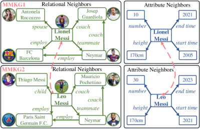
Figure 1. The MMEA task between MMKG1 and MMKG2, aligning the entities Lionel Messi and Leo Messi.

Knowledge graphs (KGs), such as DBpedia (Lehmann et al., 2015) and YAGO (Mahdisoltani et al., 2015), employ a graph structure to organize real-world factual knowledge. They provide the backbone of various web-based applications like query answering (Zhang et al., 2021; Hu et al., 2022; Nguyen et al., 2023) and search (Nguyen et al., 2019; Gu et al., 2019). Recently, several works have extended KGs with additional modeling capabilities, as required by different applications. Multi-modal Knowledge Graphs (MMKGs) extend traditional KGs with multi-modal information, e.g. visual information. However, like traditional KGs, MMKGs suffer from incompleteness and low coverage. Thus, the integration of independently developed MMKGs is paramount. A key task for MMKG integration is multi-modal entity alignment (MMEA), which aims to identify equivalent entity pairs in different MMKGs by taking into account the structure of MMKGs, as well as the attribute and visual information of entities, see e.g. Fig. 1. In this way, MMEA facilitates the exchange of knowledge among different MMKGs.

A wide variety of approaches to MMEA have been already introduced. Initial proposals (Liu et al., 2019; Chen et al., 2020; Liu et al., 2021; Guo et al., 2021) concentrated on the construction of distinct multi-modal fusion modules to integrate entity representations from multiple modalities into joint embeddings and then use aggregated embeddings to predict alignments. A shortcoming of these methods is that they only explore the use of diverse multi-modal representations to enhance the contextual embedding of entities, overlooking the capabilities of inter-modal representations to capture certain types of interactions. To overcome this, some works (Chen et al., 2022b, a; Lin et al., 2022) use siamese networks, transformer mechanisms or contrastive learning strategies to enhance multi-modal knowledge by exploiting inter-modal interaction. However, existing frameworks for MMEA still suffer from serious shortcomings:

1. Modality Distinctiveness. Existing methods have difficulties to explicitly distinguish the importance of each modality. In fact, among all modalities, the structural modal knowledge is the most prevalent. For instance, the FB15K-DB15K dataset has a total of 714,720 structural triples, while it only has 1,624 relation categories, 341 attribute categories, and 26,281 images. Whether we look at the provided data ratios or the results of ablation experiments, it is evident that the structural modality provides a richer source of knowledge and therefore deserves more attention.

2. Modality Interaction Diversity. Existing models place more emphasis on the interaction between uni-modal embeddings while overlooking interactions between uni-modal and joint-modal embeddings, leading to a lack of diversity in modality interactions. We advocate that, in practice, it is necessary to design mechanisms that better capture the interaction between uni-modal and joint-modal embeddings to fully harness the potential of all available modalities. Indeed, the interaction between the joint-modal and uni-modal representations enables simultaneous interactions with more than two modalities, covering the information gaps left by only looking at pairwise interactions.

To address the above two shortcomings, we propose the method MIMEA, a Multi-Grained Interaction framework for Multi-Modal Entity Alignment. Specifically, MIMEA includes the following four modules. The Multi-modal Knowledge Embedding module utilizes multiple individual encoders to obtain modality-specific representations for each entity. To effectively combine multi-modal knowledge, the Probability-guided Modal Fusion module takes structural knowledge as the core, and employs a probability distribution mechanism to integrate uni-modal information into joint-modal representations. Furthermore, we introduce an Optimal Transport Modal Alignment module to capture the interaction between uni-modal and joint-modal embeddings. The integration of the Probability-guided Modal Fusion and the Optimal Transport Modal Alignment modules realizes inter-modal interactions between uni-modal and joint-modal embeddings. Moreover, we introduce an intra-modal contrastive loss to distinguish the embeddings of equivalent entities from those of non-equivalent ones, for each modality. In summary, our main contributions are:

• We propose a framework to address the multi-modal entity alignment task by introducing multi-grained interaction mechanisms into the multi-modal knowledge representation process.

• We design mechanisms to explore intra-modal relationships and inter-modal interactions, ensuring that the aligned entities are semantically close.

• We conduct extensive experiments on two real-world datasets, showing the strong performance of MIMEA.

2. Related Work

Entity Alignment. Entity alignment (EA), which aims to identify equivalent entities across different knowledge graphs, is a fundamental data integration task. Existing research focuses on learning embeddings of entities by utilizing the structural information of KGs. Approaches to EA can be divided into two categories: KGE-based methods and GNN-based methods. KGE-based methods ‘move’ entity embeddings from different KGs into a unified latent space and measure the alignment by calculating the distance between entity embeddings, such as MTransE (Chen et al., 2017), JAPE (Sun et al., 2017), IPTransE (Zhu et al., 2017), BootEA (Sun et al., 2018), RNM (Zhu et al., 2021a) and NeoEA (Guo et al., 2022). Recently, GNN-based models have achieved remarkable performance in graph learning. Based on this, some works develop GNN-based frameworks for EA, such as KDCoE (Chen et al., 2018), AliNet (Sun et al., 2020), MuGNN (Cao et al., 2019), AttrGNN (Liu et al., 2020). However, all the discussed methods ignore the multi-modal knowledge (especially the visual information) available in the knowledge graph.

Multi-Modal Entity Alignment. Recently various multi-modal knowledge graphs have become available (Liu et al., 2021, 2019). Thus many works have investigated how to effectively incorporate visual knowledge into the entity alignment task. PoE (Liu et al., 2019) combines all multi-modal features into a single vector, and measures the trustworthiness of entity pairs by matching their underlying semantics. However, it cannot capture the potential interactions among different modalities. MMEA (Chen et al., 2020) integrates knowledge from different modalities into a joint representation and then calculates a similarity score between the holistic embeddings of aligned entities. EVA (Liu et al., 2021) introduces an iterative learning strategy to expand the set of training seeds. HMEA (Guo et al., 2021) encodes the multi-modal knowledge into the hyperbolic space, and uses aggregated embeddings to predict alignments. MSNEA (Chen et al., 2022b) integrates visual features to guide the learning process of relation features and adaptively assigns attention weights to capture valuable attributes for alignment. MCLEA (Lin et al., 2022) explores intra-modal and inter-modal interactions via contrastive learning to reduce the gap between modalities. MEAformer (Chen et al., 2022a) proposes a transformer-based model which can dynamically predict relativized mutual weights among modalities for each entity, encoraging the emergence of adaptive modality preferences. ACK-MMEA (Li et al., 2023) designs a multi-modal attribute uniformization module to incorporate the consistent alignment knowledge. GEEA (Guo et al., 2023) studies embedding-based entity alignment from a perspective of generative models. It converts an entity from one knowledge graph to the other one, and generates new entities from random noise vectors. However, the aforementioned methods have the following two shortcomings: On one hand, the majority of methods, such as MMEA, EVA, HMEA, and MSNEA, have not been able to fully achieve multi-granular interactions within and across modalities. Consequently, they do not effectively integrate multimodal knowledge related to entities. On the other hand, even when some methods, like MCLEA and MEAformer, introduce mechanisms for intra-modality and inter-modality interactions, they are difficult to explicitly distinguish the importance of each modality, and also ignore the interaction between uni-modal and joint-modal embeddings, which results in a lack of diversity in modal interactions.

Optimal Transport. Optimal transport (OT) is a fundamental mathematical tool which aims to derive an optimal plan to transfer one distribution to another. OT has been used in many applications, such as, computer vision (Bonneel et al., 2011; Solomon et al., 2015), domain adaption (Gu et al., 2022; Chang et al., 2022), and unsupervised learning (Caron et al., 2020; Asano et al., 2020). OTKGE (Cao et al., 2022) models the multi-modal fusion procedure as a transport plan moving different modal embeddings to a unified space by minimizing the Wasserstein distance between multi-modal distributions. MOTCat (Xu and Chen, 2023) proposes a multi-modal optimal transport-based co-attention transformer framework with global structure consistency for selecting informative patches. However, existing studies lack a comprehensive investigation of the correlations between uni-modal and joint-modal contexts. To the best of our knowledge, we are the first to adopt the optimal transport mechanism for MMEA task.

3. Preliminaries

Multi-modal Knowledge Graph. Let $\mathcal{E},\mathcal{R},\mathcal{A},\mathcal{I},\mathcal{V}$ respectively be finite sets of entities, relation types, attribute types, images, and values. A multi-modal knowledge graph (MMKG) $\mathcal{G}$ is defined as $\{\mathcal{P},\mathcal{T}_{r},\mathcal{T}_{a}\}$, where $\mathcal{P}=\{(e,i)\mid e\in\mathcal{E},i\in\mathcal{I}\}$ is the set of entity-image pairs, $\mathcal{T}_{r}=\{(h,r,t)\mid h,t\in\mathcal{E},r\in\mathcal{R}\}$ is the set of relational triples, and $\mathcal{T}_{a}=\{(e,a,v)\mid e\in\mathcal{E},a\in\mathcal{A},v\in\mathcal{V}\}$ is the set of attribute triples.

Multi-modal Entity Alignment. The aim of the multi-modal entity alignment (MMEA) task is to identify pairs of entities in two multi-modal knowledge graphs which are equivalent. Concretely, given two MMKGs $\mathcal{G}=\{\mathcal{P},\mathcal{T}_{r},\mathcal{T}_{a}\}$ and $\mathcal{G}^{\prime}=\{\mathcal{P}^{\prime},\mathcal{T}_{r}^{\prime},\mathcal{T}_{a}^{\prime}\}$, we aim to find entity pairs $\mathcal{H}=\{(e_{i},e_{j})\mid e_{i}\in\mathcal{E},e_{j}\in\mathcal{E}^{\prime},e_{i}\equiv e_{j}\}$, where $\equiv$ represents the equivalence of two entities. Usually, we will select a small set of pre-aligned entity pairs $\mathcal{S}$ (seeds) for training, to learn entity representations in the two input MMKGs.

4. Framework

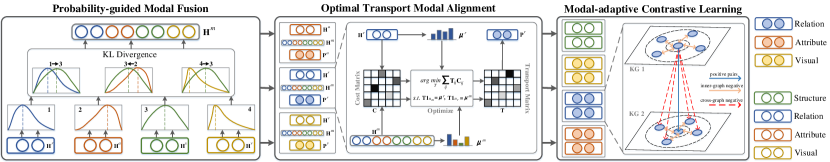
Figure 2. MIMEA’s architecture, containing the modules: Probability-guided Modal Fusion, Optimal Transport Modal Alignment, and Modal-adaptive Contrastive Learning.

We now introduce the MIMEA framework (cf. Fig 2 for its architecture), which comprises four major components (cf. Sections 4.1-4.4).

4.1. Multi-modal Knowledge Embedding

We define entity embeddings for four modalities: structural, relation, attribute and visual. Structural embeddings are obtained based on the attribute and relational neighbors (described by attribute/relational triples) of an entity. Relation embeddings are derived from relation types, and they are expressed in the form of bag-of-words. Attribute embeddings are obtained analogously. Visual embeddings are derived from entity-image pairs.

Structural Embeddings. The graph attention network (GAT) (Velickovic et al., 2018) is an attention-based architecture which has been shown to effectively encode graph-like data. We thus leverage GAT to model the structural information of $\mathcal{G}$ and $\mathcal{G}^{\prime}$. For the hidden state $\textit{{h}}_{i}\in\mathbb{R}^{d}$ ($d$ represents the embedding dimension) of entity $e_{i}$, the aggregation of its one-hop neighbors $\mathcal{N}_{i}$ with self-loops is formulated as:

(1) $$\textit{{h}}_{i}=\sigma\left(\sum_{j\in\mathcal{N}_{i}}{\alpha_{ij}\textbf{W}_{s}\textit{{h}}_{j}}\right)$$

where $\sigma(\cdot)$ denotes the nonlinear ReLU function; $\textbf{W}_{s}\in\mathbb{R}^{d\times d}$ denotes a parameterized weight matrix (Li et al., 2019; Lin et al., 2022) — we restrict $\textbf{W}_{s}$ to a diagonal matrix to reduce the number of computations; $\textit{{h}}_{j}$ is the hidden state of entity $e_{j}$; the attention weight $\alpha_{ij}$ measures the importance of entity $e_{j}$ for entity $e_{i}$, formulated as:

(2) $$\alpha_{ij}=\frac{\mathrm{exp}\left(\mathrm{LeakyReLU}\left(\textbf{a}^{\top}[\textbf{W}_{s}\textit{{h}}_{i}\parallel\textbf{W}_{s}\textit{{h}}_{j}]\right)\right)}{\sum_{k\in\mathcal{N}_{i}}{\mathrm{exp}\left(\mathrm{LeakyReLU}\left(\textbf{a}^{\top}[\textbf{W}_{s}\textit{{h}}_{i}\parallel\textbf{W}_{s}\textit{{h}}_{k}]\right)\right)}}$$

where $\textbf{a}\in\mathbb{R}^{2d}$ is a learnable parameter, $\cdot^{\top}$ and $\parallel$ respectively represent the transposition and concatenation operations. To stabilize the learning process of self-attention, we introduce a multi-head strategy (Li et al., 2019; Lin et al., 2022; Chen et al., 2022a) to generate K independent representations based on the transformation of Equation  1. Then, we concatenate these features to obtain the structural embedding $\textit{{h}}_{i}^{s}$ of entity $e_{i}$ as:

(3) $$\textit{{h}}_{i}^{s}=\mathop{\|}_{k=1}^{K}\sigma\left(\sum_{j\in\mathcal{N}_{i}}{\alpha_{ij}^{k}\textbf{W}_{s}^{k}\textit{{h}}_{j}}\right)$$

where $\alpha_{ij}^{k}$ denotes the normalized attention coefficients computed by the $k$-th attention mechanism, and $\textbf{W}_{s}^{k}$ is the corresponding input linear transformation’s weight matrix. We use a two-layer GAT to aggregate the neighborhood information across multiple hops, and use the output of the final GAT layer as the structural embedding. The structural embedding of all entities is represented as $\textbf{H}^{s}\in\mathbb{R}^{n\times d}$, where $n$ represents the number of entities in the input dataset.

Relation and Attribute Embeddings. Note that the knowledge from attribute types is coarser than that of relational types. Thus, directly mixing the representations of relations and attributes using a GAT can easily lead to the problem of information contamination (Liu et al., 2021). To alleviate this issue, we respectively regard the relations and attributes of entity $e_{i}$ as bag-of-words features $w_{i}^{r}$ and $w_{i}^{a}$. We further apply the multi-layer perceptrons $\mathrm{MLP}_{r}$ and $\mathrm{MLP}_{a}$ to respectively obtain the relation embedding $\textit{{h}}_{i}^{r}$ and attribute embedding $\textit{{h}}_{i}^{a}$, calculated as:

(4) $$\textit{{h}}_{i}^{r}=\mathrm{MLP}_{r}(w_{i}^{r}),\quad\textit{{h}}_{i}^{a}=\mathrm{MLP}_{a}(w_{i}^{a})$$

The relation and attribute embedding of all entities are respectively represented as $\textbf{H}^{r}\in\mathbb{R}^{n\times d}$ and $\textbf{H}^{a}\in\mathbb{R}^{n\times d}$.

Visual Embeddings. VGG (Simonyan and Zisserman, 2015) are usually pre-trained on large-scale image datasets and can extract useful features from images that are beneficial to different visual tasks. In practice, we feed the image $v_{i}$ of entity $e_{i}$ into the VGG-16 encoder $\mathrm{Enc}_{v}$. We use the final layer output before logits as the visual feature, and finally apply a multi-layer perceptron $\mathrm{MLP}_{v}$ to obtain the visual embedding $\textit{{h}}_{i}^{v}$:

(5) $$\textit{{h}}_{i}^{v}=\mathrm{MLP}_{v}(\mathrm{Enc}_{v}(v_{i}))$$

The visual embedding of all entities is represented as $\textbf{H}^{v}\in\mathbb{R}^{n\times d}$.

4.2. Probability-guided Modal Fusion

Different modalities concentrate on different types of knowledge. Thus, each modality contributes differently to the characterization of specific aspects of an entity. Typically, it is required to combine multiple modalities of knowledge to provide a more comprehensive understanding of an entity. For example, knowledge about the entity Lionel Messi includes the relational triple (Lionel Messi, employ, FC Barcelona) and a visual image (an image of Messi wearing a certain team’s jersey). So, when evaluating the football club Lionel Messi plays for, the structural knowledge from the relational triple is more relevant than the knowledge from the image. However, when it comes to Messi’s jersey number at a club, the triple (Lionel Messi, employ, FC Barcelona) does not contain relevant information, but a visual image of Messi wearing a 10 jersey can provide more appropriate clues. Holistically combining these two types of information will thus enable an accurate representation of the football club Lionel Messi plays for and his jersey number at that club. Therefore, an important challenge is how to better integrate multi-modal knowledge to obtain effective fused representations in multi-modal contexts.

A key source of knowledge in multi-modal knowledge graphs is the one provided by structural triples. The structural triples contain the relational triples and attribute triples, they can provide a more direct representation of the content of an entity and its relationship with other entities. For example, in the FB15K-DB15K dataset, there are a total of 714,720 structural triples, resulting in richer knowledge about the connections among entities. In contrast, the FB15K-DB15K dataset contains only 1,624 relational types and 341 attribute types, which means that the initialization vectors for the relation and attribute modalities will be bag-of-words vectors of length 1,624 and 341. Consequently, the representation of relation and attribute modalities of an entity lacks sufficient distinctiveness. Indeed, in subsequent ablation experiments we will show that the structural content has the most significant impact on the final performance of entity alignment. Therefore, using structural embeddings as a pivotal point, we introduce the Probability-guided Modal Fusion (PMF) module, which employs a probabilistic distribution to achieve initial interactions between relation embeddings and structural embeddings, attribute embeddings and structural embeddings, also visual embeddings and structural embeddings. It generates interactive weights in the first stage and aggregates different modal embeddings to obtain a joint-modal combined representation based on these weight coefficients. Specifically, the PMF module comprises the following three steps:

1. Constructing Probability Distributions. Given the structural embedding $\textbf{H}^{s}$, relation embedding $\textbf{H}^{r}$, attribute embedding $\textbf{H}^{a}$, and visual embedding $\textbf{H}^{v}$ of all entities, we represent each embedding using a probability density form based on the Beta probability distribution function. The Beta distribution has two shape hyperparameters $\alpha$ and $\beta$. Its probability density function (PDF) is defined as: $f_{(\alpha,\beta)}(x)=\frac{x^{\alpha-1}(1-x)^{\beta-1}}{\textbf{B}(\alpha,\beta)}$, where $x\in[0,1]$ and $\textbf{B}(\cdot)$ denotes the Beta function. To transform, for example, the structural embedding $\textbf{H}^{s}$ into a Beta distribution, we proceed as follows: i) we first divide $\textbf{H}^{s}$ into two equal parts $\boldsymbol{\alpha}^{s}$ and $\boldsymbol{\beta}^{s}$ according to the embedding dimension: $\textbf{H}^{s}=\{[\boldsymbol{\alpha}^{s},\boldsymbol{\beta}^{s}]\,|\,\boldsymbol{\alpha}^{s}\in\mathbb{R}^{n\times m},\boldsymbol{\beta}^{s}\in\mathbb{R}^{n\times m},m=\frac{d}{2}\}$. Then, we use each part as a shape parameter of the Beta distribution. ii) By combining the i-th element $\alpha^{s}_{i}$ in $\boldsymbol{\alpha}^{s}$ with the i-th element $\beta^{s}_{i}$ in $\boldsymbol{\beta}^{s}$, we will form the i-th Beta distribution. The combination of all elements will form m Beta distributions, represented as $\mathcal{D}^{s}=[(\alpha^{s}_{1},\beta^{s}_{1}),\ldots,(\alpha^{s}_{m},\beta^{s}_{m})]$. We denote the PDF of the i-th Beta distribution in $\mathcal{D}^{s}$ as $p_{i}^{s}$. iii) We can analogously get the Beta distributions of the relation, attribute and visual embedding: $\mathcal{D}^{r}$, $\mathcal{D}^{a}$, $\mathcal{D}^{v}$, and the corresponding i-th Beta distributions: $p_{i}^{r}$, $p_{i}^{a}$, and $p_{i}^{v}$.

2. Calculating Modal Weight Coefficients. Given the relation and structural embedding’s Beta distributions $\mathcal{D}^{r}$ with parameters $[(\alpha^{r}_{1},\beta^{r}_{1}),...,(\alpha^{r}_{m},\beta^{r}_{m})]$ and $\mathcal{D}^{s}$ with corresponding parameters $[(\alpha^{s}_{1},\beta^{s}_{1}),...,(\alpha^{s}_{m},\beta^{s}_{m})]$, we define the distance between the relation and structural embedding as the sum of the KL divergence between the two Beta distributions along each dimension:

   (6) $$\delta_{(r,s)}=\sum_{i=1}^{m}{\mathrm{KL}(p_{i}^{r},p_{i}^{s})}$$

   Then, we convert the KL distance $\delta_{(r,s)}$ to a weight coefficient based on $w_{(r,s)}=\lambda(2-\delta_{(r,s)})^{2}$, where $\lambda$ represents the incremental rate, set empirically. Using the same method, we can obtain the weight coefficient $w_{(a,s)}$ between the attribute and structural embedding, and the weight coefficient $w_{(v,s)}$ between the visual and structural embedding.

3. Fusing Different Modal Embeddings. We add the three weight coefficients $w_{(r,s)}$, $w_{(a,s)}$, $w_{(v,s)}$ with the initialized value 1.0 (initially we assume that all modalities have the same weight coefficients) and normalize it to obtain the prior assumption: $W_{\text{PMF}}=\textit{softmax}([w_{(r,s)},w_{(a,s)},w_{(v,s)}]+1.0$). Then, we multiply these weight coefficients with the embedding representation of the corresponding modality, and concate the multiplied results to obtain the final fused modality representation $\textbf{H}^{m}\in\mathbb{R}^{n\times 4d}$.

4.3. Optimal Transport Modal Alignment

The PMF deals with various modalities of knowledge by combining multimodal information. However, due to the introduced noise during the fusion process, an optimal representation of an entity cannot be based only on joint-modal information. For instance, if we are interested in the football club in which Lionel Messi plays, given the joint-modal embedding incorporating the relational triple (Lionel Messi, employ, FC Barcelona), the attribute triple (Lionel Messi, number, 10) and the visual image of Messi wearing the Barcelona jersey number 10, the knowledge provided by the attribute triple is regarded as noise, while the one provided by the relational triple is useful information. Therefore, in some cases, while using joint-modal embeddings, we need to retain the knowledge of individual embeddings for each modality to assess the extent to which a single modality represents an entity in a certain context. So, a natural question is how to achieve better interaction between uni-modal and joint-modal embeddings to cover the information gap of single modalities and reduce the noise of joint-modal embeddings?

Optimal transport (OT) aims to transport the density distribution of a group of elements to that of another group with minimal total cost. To consider the correlations of uni-modal and joint-modal representations, we can regard uni-modal as one group elements and joint-modal as another group elements. The expectation is that the uni-modal and joint-modal elements have an appropriate correlation with minimal total transportation cost. To achieve this, we first generate an intermediate transition matrix by aligning and optimizing uni-modal and joint-modal embeddings. Subsequently, by combining uni-modal information with the generated intermediate transition matrix, we obtain an enriched uni-modal embedding. The Optimal Transport Modal Alignment (OTMA) module consists of the following steps:

1. Building the Transport Task. We look, for instance, at how to obtain the intermediate modal embedding between the relation modal embedding $\textbf{H}^{r}$ and the joint modal embedding $\textbf{H}^{m}$. Optimal transport aims at computing a minimal cost transportation between a source distribution $\mu^{r}$ and a target distribution $\mu^{m}$:

   (7) $$\mu^{r}=\sum_{i=1}^{n_{r}}{q_{i}^{r}\varphi(x_{i})},\,\,\,\mu^{m}=\sum_{i=1}^{n_{m}}{q_{i}^{m}\varphi(y_{i})}$$

   where $\mu^{r}$ and $\mu^{m}$ are defined on the probability space $\textbf{H}^{r}$ and $\textbf{H}^{m}$, $\varphi(\cdot)$ denotes the Dirac function, $n_{r}$ and $n_{m}$ are the number of samples, $x_{i}$ and $y_{i}$ are the i-th sample of $\textbf{H}^{r}$ and $\textbf{H}^{m}$ (in practice, to reduce the computational complexity, the number of selected samples will be lower than the embedding dimension), $q_{i}^{r}$ and $q_{i}^{m}$ are the probability mass of the i-th samples, satisfying the following conditions: $\sum_{i=1}^{n_{r}}{q_{i}^{r}}=\sum_{i=1}^{n_{m}}{q_{i}^{m}}=1$, to simplify the calculations, we set $q_{i}^{r}=\frac{1}{n_{r}}$ and $q_{i}^{m}=\frac{1}{n_{m}}$. We define a cost matrix C with $\textbf{C}_{ij}$ representing the distance (usually the cosine distance) between $x_{i}$ and $y_{j}$.

2. Optimal Transport Plan. Based on distributions $\mu^{r}$ and $\mu^{m}$, we can obtain all joint probability distributions $\Pi(\mu^{r},\mu^{m})$. Combining them with the cost matrix C, we can convert the optimal transport into the following form:

   (8) $$\mathcal{W}(\mu^{r},\mu^{m})=\underset{\textbf{T}\in\Pi(\mu^{r},\mu^{m})}{\textit{min}}\sum_{i=1}^{n_{r}}\sum_{j=1}^{n_{m}}\textbf{T}_{ij}\textbf{C}_{ij}$$

   where $\Pi(\mu^{r},\mu^{m})=\{\textbf{T}\in\mathbb{R}^{n_{r}\times n_{m}}|\textbf{T1}_{n_{m}}=\mu^{r},\textbf{T}^{\top}\textbf{1}_{n_{r}}=\mu^{m}\}$, with 1 an all-one vector, $\textbf{T}_{ij}$ the optimal amount of mass to move from $x_{i}$ to $y_{j}$ to obtain an overall minimum cost. We apply the Sinkhorn algorithm (Cuturi, 2013) to optimize Equation (8) to get the optimal transportation matrix T.

3. Translating Uni-Modal Embeddings. We multiply the relation embedding $\textbf{H}^{r}$ with the transportation matrix T to get the intermediate embedding $\textbf{P}^{r}={\textbf{H}^{r}}^{\top}\textbf{T}$ between the relation-modal embedding $\textbf{H}^{r}$ and the joint-modal embedding $\textbf{H}^{m}$. The resulting embedding focuses on relational modal knowledge, but can also be aligned with joint modal embeddings at a small cost.

We can analogously obtain attribute and visual intermediate embeddings, denoted as $\textbf{P}^{a}$ and $\textbf{P}^{v}$, respectively. We found that there is no need to align the structural-modal embedding with the joint-modal embedding since the structural embedding in the joint embedding has the largest weight and therefore dominates the joint embedding.

4.4. Modal-adaptive Contrastive Learning

The OTMA module focuses on the interaction between uni-modal and joint-modal aspects of knowledge. However, both the OTMA and PMF modules overlook the interactions within a single modality. In many cases, for a given entity, there exist multiple associated pieces of information within a single modality. When predicting a specific attribute of an entity, typically only a subset of these related pieces of knowledge plays a decisive role. For instance, consider the entity Lionel Messi, which includes the relational triples: (Lionel Messi, spouse, Antonela Roccuzzo) and (Lionel Messi, child, Thiago Messi) related to family relationships and (Lionel Messi, teammate, Neymar) and (Lionel Messi, coach, Josep Guardiola) related to player attributes. Clearly, when describing Messi’s family relationships, Antonela Roccuzzo and Thiago Messi are more important than Neymar and Josep Guardiola. However, when discussing Messi’s football career, the situation is reversed. Therefore, it is preferable to make the embeddings of Antonela Roccuzzo and Thiago Messi closer in the embedding space, while the embeddings of Antonela Roccuzzo and Neymar should be pushed farther apart. Based on these observations, an important challenge is how to enforce embeddings to respect modal properties, while distinguishing the embedding of an entity from those of other entities, for each modality.

Inspired by the contrastive learning mechanism (Zolfaghari et al., 2021; Lin et al., 2022; Zhu et al., 2021b), we devise a Modal-adaptive Contrastive Learning (MCL) module, which maps inner-graph aligned pairs to a proximate location, but also pushes the inner-graph and cross-graph unaligned pairs father apart. Specifically, MCL includes the following three parts:

• Creating Positive and Negative Samples. Following a 1-to-1 alignment constraint (Lin et al., 2022; Chen et al., 2022a), the entity pairs within the seed alignments $\mathcal{S}$ can be naturally regarded as positive samples, whereas any non-aligned pairs can be regarded as negative samples. Let ($e_{i}^{1},e_{i}^{2}$) in $\mathcal{S}$ (with $e_{i}^{1}\in\mathcal{G}$ and $e_{i}^{2}\in\mathcal{G}^{\prime}$) be the i-th aligned entity pair, the negative samples of $e_{i}^{1}$ are obtained from two sources: the inner-graph unaligned pairs from $\mathcal{G}$ and cross-graph unaligned pairs from $\mathcal{G}^{\prime}$. More precisely, they are defined as $\mathcal{N}_{i}^{1}=\{e_{j}^{1}~{}|~{}\forall e_{j}^{1}\in\mathcal{G},j\neq i\}$ and $\mathcal{N}_{i}^{2}=\{e_{j}^{2}~{}|~{}\forall e_{j}^{2}\in\mathcal{G}^{\prime},j\neq i\}$. It should be noted that we use the in-batch negative sampling strategy (Lin et al., 2022; Chen et al., 2022a) to limit the negative sample scope within the mini-batch.

• Contrastive Learning Loss. For the constructed positive and negative examples, we perform contrastive learning under each modal condition. For instance, for the relational modality, we construct the contrastive learning loss $\mathcal{L}^{r}(e_{i}^{1},e_{i}^{2})$ of the positive pair ($e_{i}^{1},e_{i}^{2}$) as:

  (9) $$-\mathrm{log}\frac{\theta(e_{i}^{1},e_{i}^{2})}{\theta(e_{i}^{1},e_{i}^{2})+\gamma\,\sum_{e_{j}^{1}\in\mathcal{N}_{i}^{1}}{\theta(e_{i}^{1},e_{j}^{1})}+\sum_{e_{j}^{2}\in\mathcal{N}_{i}^{2}}{\theta(e_{i}^{1},e_{j}^{2})}}$$

  where $\theta(x,y)=exp(f_{r}(x)^{\top}f_{r}(y)/\tau)$, $f_{r}(\cdot)$ is the relation encoder, $\tau$ is a temperature parameter, and $\gamma$ is a hyper-parameter to control inner-graph alignment. The second and third terms in the denominator sum up inner-graph and cross-graph negative samples, respectively. We apply L2-normalisation to the input feature embeddings before computing the inner product (Zolfaghari et al., 2021; Lin et al., 2022; Suh et al., 2019). Similarly, we can obtain the loss for the other direction as $\mathcal{L}^{r}(e_{i}^{2},e_{i}^{1})$. The final contrastive loss of the relational modality is the average of the losses in the two directions, expressed as: $\mathcal{L}^{r}=\frac{1}{2}[\mathcal{L}^{r}(e_{i}^{1},e_{i}^{2})+\mathcal{L}^{r}(e_{i}^{2},e_{i}^{1})]$.

• Optimization Objective. Using the same idea, we can obtain the contrastive loss of structural, attribute, visual and joint modalities, respectively expressed as $\mathcal{L}^{s}$, $\mathcal{L}^{a}$, $\mathcal{L}^{v}$, and $\mathcal{L}^{m}$. The overall loss is defined as:

  (10) $$\mathcal{L}=\sum_{\ell\in\mathcal{M}}{\phi^{\ell}\mathcal{L}^{\ell}},\,\,\mathcal{M}=\{s,r,a,v,m\}$$

  where $\phi^{\ell}$ is the hyper-parameter that balances the importance of different modal losses. Similar to (Kendall et al., 2018), we introduce a multi-task learning paradigm and then use homoscedastic uncertainty to weight each loss automatically during model training. Details of this strategy can be found in (Kendall et al., 2018). It should be noted that only the MCL module has loss values, and the PMF and OTMA modules do not have any loss content.

5. Experiments

Table 1. Evaluation of different models in the non-iterative setting. Results marked with $\dagger$, $\ddagger$ and $\ast$ respectively come from (Lin et al., 2022) (Chen et al., 2022a), and the corresponding paper. Best scores are in bold, the second best scores are underlined, and ‘–’ indicates the results are not reported in previous work.

Methods	FB15K-DB15K									FB15K-YAGO15K
	20%			50%			80%			20%			50%			80%
	MRR	H@1	H@10	MRR	H@1	H@10	MRR	H@1	H@10	MRR	H@1	H@10	MRR	H@1	H@10	MRR	H@1	H@10
PoE (Liu et al., 2019)†	0.170	0.126	0.251	0.533	0.464	0.658	0.721	0.666	0.820	0.154	0.113	0.229	0.414	0.347	0.536	0.635	0.573	0.746
HMEA (Guo et al., 2021)†	–	0.127	0.369	–	0.262	0.581	–	0.417	0.786	–	0.105	0.313	–	0.265	0.581	–	0.433	0.801
MMEA (Chen et al., 2020)†	0.357	0.265	0.541	0.512	0.417	0.703	0.685	0.590	0.869	0.317	0.234	0.480	0.486	0.403	0.645	0.682	0.598	0.839
EVA (Liu et al., 2021)‡	0.283	0.199	0.448	0.422	0.334	0.589	0.563	0.484	0.696	0.224	0.153	0.361	0.388	0.311	0.534	0.565	0.491	0.692
MSNEA (Chen et al., 2022b)‡	0.175	0.114	0.296	0.388	0.288	0.590	0.613	0.518	0.779	0.153	0.103	0.249	0.413	0.320	0.589	0.620	0.531	0.778
MCLEA (Lin et al., 2022)‡	0.393	0.295	0.582	0.637	0.555	0.784	0.790	0.735	0.890	0.332	0.254	0.484	0.574	0.501	0.705	0.722	0.667	0.824
MEAformer (Chen et al., 2022a)‡	0.518	0.417	0.715	0.698	0.619	0.843	0.820	0.765	0.916	0.417	0.327	0.595	0.639	0.560	0.778	0.766	0.703	0.873
ACK-MMEA (Li et al., 2023)∗	0.387	0.304	0.549	0.624	0.560	0.736	0.752	0.682	0.874	0.360	0.289	0.496	0.593	0.535	0.699	0.744	0.676	0.864
GEEA (Guo et al., 2023)∗	0.450	0.343	0.661	0.723	0.651	0.852	0.836	0.787	0.918	0.393	0.298	0.585	0.668	0.589	0.808	0.790	0.733	0.890
MIMEA	0.594	0.506	0.756	0.748	0.683	0.861	0.841	0.799	0.914	0.506	0.417	0.671	0.692	0.622	0.818	0.795	0.741	0.884

To evaluate the effectiveness of MIMEA, we aim to explore the following research questions:

• RQ1 (Effectiveness): How does MIMEA perform compared to the SoTA?

• RQ2 (Ablation studies): How do different components of MIMEA contribute to its performance?

• RQ3 (Complexity analysis): What is the amount of computation and parameters used by MIMEA?

• RQ4 (Parameter analysis): How do hyper-parameters influence the performance of MIMEA? A detailed analysis can be found in Appendix D.

5.1. Experimental Setup

Datasets. We evaluate the MIMEA model on two well-known datasets: FB15K-DB15K and FB15K-YAGO15K, which include 12,846 and 11,199 alignment pairs, respectively. As in previous works (Chen et al., 2022a; Lin et al., 2022; Li et al., 2023), to evaluate MIMEA’s performance under different conditions, we split the two datasets into training and testing sets with 20%, 50%, and 80% of pre-aligned pairs given as alignment seeds. The statistics of these datasets can be found in Appendix A.

Iterative Training. As in previous works (Liu et al., 2021; Chen et al., 2022b; Lin et al., 2022; Chen et al., 2022a), we adopt a probation strategy for iterative training. Specifically, we constructed a buffer to temporarily store entity pairs that are close in the embedding space across different knowledge graphs. In every round $R$, we select entity pairs that meet the nearest distance criteria and add them to the buffer. If after $M$ iterations, these entity pairs are still in the buffer, we will add them to the training set. This approach effectively serves as a data augmentation strategy during training, where the entity pairs in the buffer can be considered as pseudo-labels. In contrast, the training method that does not involve the aforementioned iterative process is referred to as non-iterative training.

Baselines. In the experiments, we used two training strategies: non-iterative and iterative training. For each training strategy, we used different baselines. For non-iterative training: PoE (Liu et al., 2019), HMEA (Guo et al., 2021), MMEA (Chen et al., 2020), EVA (Liu et al., 2021), MSNEA (Chen et al., 2022b), MCLEA (Lin et al., 2022), MEAformer (Chen et al., 2022a), ACK-MMEA (Li et al., 2023), and GEEA (Guo et al., 2023). For iterative training: EVA (Liu et al., 2021), MSNEA (Chen et al., 2022b), MCLEA (Lin et al., 2022), and MEAformer (Chen et al., 2022a). Implementation details and evaluation metrics can respectively be found in Appendix B and C.

5.2. Main Results

To address RQ1, we conduct experiments on the non-iterative and iterative training settings, and on the number of selected pre-aligned seeds. The results are shown in Tables 1 and 2.

Performance Comparison. We can observe in the results that under both the non-iterative and iterative settings, MIMEA generally outperforms existing SoTA baselines by a large margin across all metrics. More precisely, we have the following observations. On the one hand, MIMEA achieves the best performance on the multi-modal entity alignment task. For example, in the non-iterative setting, on the FB15K-YAGO15K dataset, MIMEA achieves improvements of 8.9%, 2.4% and 0.5% on MRR compared to the best SoTA baselines when the given pre-aligned seeds are 20%, 50%, and 80%, respectively. Similar improvements are obtained on the FB15K-DB15K dataset. On the other hand, the iterative training strategy can significantly improve model performance of existing baselines and MIMEA. For example, on the FB15K-DB15K dataset when the given pre-aligned seeds are 20%, 50%, and 80%, depending on whether MIMEA uses the iterative training mechanism, there will be fluctuations of 10%, 2.2%, and 1.4% on MRR, respectively. This is primarily attributed to the generation of pseudo-entity alignments pairs during the iterative training process, which iteratively filters out potentially wrong entity pairs.

Table 2. Evaluation of different models under iterative setting. $\ddagger$ results come from  (Chen et al., 2022a). $\ast$ results from the corresponding papers. Best scores are highlighted in bold, the second best scores are underlined.

Methods	FB15K-DB15K									FB15K-YAGO15K
	20%			50%			80%			20%			50%			80%
	MRR	H@1	H@10	MRR	H@1	H@10	MRR	H@1	H@10	MRR	H@1	H@10	MRR	H@1	H@10	MRR	H@1	H@10
EVA (Liu et al., 2021)‡	0.318	0.231	0.488	0.449	0.364	0.606	0.573	0.491	0.711	0.260	0.188	0.403	0.404	0.325	0.560	0.572	0.493	0.695
MSNEA (Chen et al., 2022b)‡	0.232	0.149	0.392	0.459	0.358	0.656	0.651	0.565	0.810	0.210	0.138	0.346	0.472	0.376	0.646	0.668	0.593	0.806
MCLEA (Lin et al., 2022)∗	0.534	0.445	0.705	0.652	0.573	0.800	0.784	0.730	0.883	0.474	0.388	0.641	0.616	0.543	0.759	0.715	0.653	0.835
MEAformer (Chen et al., 2022a)‡	0.661	0.578	0.812	0.755	0.690	0.871	0.834	0.784	0.921	0.529	0.444	0.692	0.682	0.612	0.808	0.783	0.724	0.880
MIMEA	0.694	0.622	0.824	0.770	0.716	0.872	0.855	0.821	0.919	0.587	0.513	0.729	0.712	0.651	0.827	0.803	0.757	0.885

Table 3. Ablation studies under different modals and different modules. Best scores are highlighted in bold.

Settings	FB15K-DB15K									FB15K-YAGO15K
	20%			50%			80%			20%			50%			80%
	MRR	H@1	H@10	MRR	H@1	H@10	MRR	H@1	H@10	MRR	H@1	H@10	MRR	H@1	H@10	MRR	H@1	H@10
w/o structure	0.094	0.044	0.183	0.134	0.066	0.264	0.220	0.117	0.447	0.088	0.051	0.151	0.105	0.056	0.192	0.175	0.094	0.335
w/o attribute	0.664	0.589	0.806	0.750	0.694	0.859	0.839	0.801	0.910	0.553	0.479	0.700	0.684	0.620	0.806	0.774	0.718	0.871
w/o relation	0.642	0.565	0.785	0.742	0.685	0.850	0.831	0.791	0.902	0.507	0.429	0.660	0.661	0.587	0.801	0.776	0.717	0.875
w/o visual	0.691	0.616	0.825	0.772	0.716	0.877	0.853	0.815	0.921	0.568	0.492	0.717	0.699	0.633	0.822	0.791	0.736	0.886
1-19 w/o PMF	0.595	0.507	0.757	0.747	0.682	0.862	0.841	0.797	0.914	0.494	0.406	0.659	0.688	0.617	0.817	0.794	0.741	0.885
w/o OTMA	0.576	0.486	0.748	0.724	0.648	0.860	0.845	0.797	0.923	0.518	0.437	0.673	0.660	0.578	0.810	0.796	0.737	0.897
w/o MCL	0.630	0.535	0.797	0.744	0.671	0.873	0.844	0.802	0.918	0.535	0.449	0.690	0.680	0.612	0.795	0.780	0.723	0.878
MIMEA	0.694	0.622	0.824	0.770	0.716	0.872	0.855	0.821	0.919	0.587	0.513	0.729	0.712	0.651	0.827	0.803	0.757	0.885

Impact of Number of Pre-aligned Seeds. We evaluate the sensitivity of MIMEA to the given number of pre-aligned seeds: 20%, 50%, and 80% (Liu et al., 2021; Chen et al., 2022b; Lin et al., 2022; Chen et al., 2022a). From the results, we can observe that MIMEA achieves the best performance on both the FB15K-DB15K and the FB15K-YAGO15K datasets in all metrics and proportions, confirming its robustness to the number of given pre-aligned seeds. For instance, in the iterative setting, on FB15K-YAGO15K, compared with the best-performing baseline MEAformer, for 20%, 50%, and 80%, the MRR metric is respectively improved by 5.8%, 3.0% and 2.0%. The higher improvement for 20% shows that MIMEA is well-suited for low-resource scenarios. This is mainly because, on the one hand, each modality can be explicitly given a differentiation weight according to the characteristics of such modality. Further, we take into account the interactions between uni-modal and joint-modal representations. On the other hand, intra-modal is able to differentiate uni-modal representations. The intra-modal and inter-modal multi-granularity interaction can indeed maximize the utility of having multi-modal knowledge.

5.3. Ablation Studies

We address RQ2 from four perspectives, including different variants, different modalities, different distribution methods, and different pivotal modality. The results are shown in Tables 3,  4, and 5.

Table 4. Evaluation of different models under different distribution methods. Best scores are highlighted in bold.

Settings	FB15K-DB15K									FB15K-YAGO15K
	20%			50%			80%			20%			50%			80%
	MRR	H@1	H@10	MRR	H@1	H@10	MRR	H@1	H@10	MRR	H@1	H@10	MRR	H@1	H@10	MRR	H@1	H@10
Beta	0.694	0.622	0.824	0.770	0.716	0.872	0.855	0.821	0.919	0.587	0.513	0.729	0.712	0.651	0.827	0.803	0.757	0.885
Cauchy	0.697	0.625	0.825	0.770	0.713	0.877	0.852	0.815	0.921	0.592	0.516	0.734	0.715	0.651	0.833	0.806	0.757	0.891
Gamma	0.691	0.621	0.822	0.769	0.713	0.874	0.851	0.818	0.915	0.575	0.496	0.724	0.708	0.646	0.828	0.802	0.751	0.893
Gumbel	0.690	0.619	0.821	0.769	0.714	0.872	0.851	0.816	0.917	0.573	0.493	0.722	0.708	0.645	0.827	0.801	0.749	0.890
Laplace	0.694	0.624	0.823	0.770	0.715	0.875	0.851	0.816	0.920	0.581	0.503	0.729	0.713	0.650	0.831	0.803	0.754	0.892

Impact of Modalities. The upper part of Table 3 shows the individual contribution of different modalities. We can observe that independent of the dataset or the number of pre-aligned seeds, the removal of different modalities has varying degrees of performance drop. The structural information has shown to be the main source, with its removal leading to the most significant drop (this is in line with previous findings (Lin et al., 2022)). This might be explained by the wealth of structural triples available in both datasets. On the other extreme, the performance gain brought by the visual modality is minimal. In fact, the removal of visual information can sometimes lead to achieve better results. The main reason is that the visual information provides limited additional knowledge. Only through the interaction with other modal information can bring certain performance improvement.

Impact of Modules. The lower part of Table 3 presents the results of the impact of each component of MIMEA on the performance. We can observe that by removing any module the performance dramatically degrades. This could be explained by the fact that different modules play different roles, realizing multi-granular modal information interaction. For example, the PMF module focuses on the interaction of uni-modal information (with the structural information as the core) and can ultimately form joint-modal representations. In contrast, the MCL module underscores the significance of intra-modal interactions for each modality. The MIMEA’s modules are interrelated and form a complete data flow, so the absence of any one of them leads to a significant performance fluctuation.

Impact of Distribution Methods. We investigate the choice of different probability distribution functions in the PMF module. Table 4 reports the results by replacing the Beta function in the PMF module with the Cauchy, Gamma, Gumbel, or Laplace functions. We observe that using different probability distribution functions has a relatively limited impact on MIMEA’s performance, showing the robustness of the PMF module. This is explained by the fact that the weight coefficients obtained by each probability distribution function tend to be similar after subsequent gradient updates.

Impact of Different Pivotal Modality. In the PMF module, we use the structural modality as the central one for the interaction between uni-modal representations. To verify the adequateness of this choice, we select attribute, relation, and visual as the central ones. The experimental results are shown in Table 5. We can observe that by choosing the structural modality as the core we achieve the best results. The main reason is that the datasets contain rich knowledge of structural triples, which can provide abundant evidence. Recall that the performance loss caused by removing the visual modality in Table 3 is lower than that of removing the relation and attribute modalities, that is, the visual modality seems to be of little importance in the MMEA task. However, when using the visual modality as the core for uni-modal interaction, it can achieve better results than the relation and attribute modalities. A possible explanation is that the subsequent OTMA module directly assists the functioning of the visual modality, because from Table 3 we find that removing the OTMA module has the largest impact on performance.

Table 5. The MRR metric results of using different modal content as the central one in the PMF module. Best scores are highlighted in bold.

Methods	FB15K-DB15K			FB15K-YAGO15K
	20%	50%	80%	20%	50%	80%
attribute	0.595	0.747	0.841	0.494	0.688	0.794
relation	0.576	0.724	0.845	0.518	0.660	0.796
visual	0.630	0.744	0.844	0.535	0.680	0.780
structural	0.694	0.770	0.855	0.587	0.712	0.803

5.4. Complexity Analysis

To address RQ3, we analyze the model’s complexity from two perspectives: time complexity and space complexity. The time complexity can be measured by the amount of model calculations, while the space complexity can be measured by the amount of model’s parameters. Model calculation volume refers to the number of floating-point operations performed during the inference process of the model, usually expressed in units of FLOPs (Floating-Point Operations Per Second). The number of model parameters refers to the number of adjustable parameters that need to be learned in the model. These parameters are the weights and biases of the model that are adjusted through optimization algorithms such as gradient descent during the training process. The number of parameters is usually expressed in “Millions” (M) or “Billions” (G). Table 6 presents the time and space complexity results of MIMEA and the best-performing MCLEA (Lin et al., 2022) and the MEAformer (Chen et al., 2022a) model. We can find that MIMEA simultaneously reduces the computational cost and the number of parameters in comparison to the other two baselines. In particular, the amount of calculation needed by MIMEA is one-third of MEAformer’s. To sum up, MIMEA can achieve the best performance while minimizing the model’s computational load and video memory footprint.

Table 6. Amount of parameters and calculations required by different models on different datasets.

Metrics	Model	FB15K-DB15K	FB15K-YAGO15K
FLOPs	MCLEA (Lin et al., 2022)	103.345G	112.872G
	MEAformer (Chen et al., 2022a)	203.100G	219.175G
	MIMEA	67.770G	74.018G
Params	MCLEA (Lin et al., 2022)	3.720M	3.720M
	MEAformer (Chen et al., 2022a)	3.461M	3.374M
	MIMEA	2.440M	2.440M

6. Conclusion and future work

In this paper, we proposed MIMEA, a framework for multi-modal entity alignment that effectively leverages multi-modal knowledge with the exploitation of intra-modal and inter-modal interactions. The experimental results demonstrate the effectiveness of MIMEA. For future work, given that the structural information is the most significant and that in practice, structural knowledge is often incomplete, we could first employ knowledge graph completion techniques to fill in missing parts.

References

- (1)
- Asano et al. (2020) Yuki Markus Asano, Mandela Patrick, Christian Rupprecht, and Andrea Vedaldi. 2020. Labelling unlabelled videos from scratch with multi-modal self-supervision. In NeurIPS. Curran Associates, online, 1–12.
- Bonneel et al. (2011) Nicolas Bonneel, Michiel van de Panne, Sylvain Paris, and Wolfgang Heidrich. 2011. Displacement Interpolation using Lagrangian Mass Transport. ACM Trans. Graph. 30, 6 (2011), 158.
- Cao et al. (2019) Yixin Cao, Zhiyuan Liu, Chengjiang Li, Zhiyuan Liu, Juanzi Li, and Tat-Seng Chua. 2019. Multi-Channel Graph Neural Network for Entity Alignment. In ACL. ACL, Florence, Italy, 1452–1461.
- Cao et al. (2022) Zongsheng Cao, Qianqian Xu, Zhiyong Yang, Yuan He, Xiaochun Cao, and Qingming Huang. 2022. OTKGE: Multi-modal Knowledge Graph Embeddings via Optimal Transport. In NeurIPS. NeurIPS Foundation, New Orleans, the United States, 1–13. http://papers.nips.cc/paper_files/paper/2022/hash/ffdb280e7c7b4c4af30e04daf5a84b98-Abstract-Conference.html
- Caron et al. (2020) Mathilde Caron, Ishan Misra, Julien Mairal, Priya Goyal, Piotr Bojanowski, and Armand Joulin. 2020. Unsupervised Learning of Visual Features by Contrasting Cluster Assignments. In NeurIPS. Curran Associates, online, 1–13.
- Chang et al. (2022) Wanxing Chang, Ye Shi, Hoang Tuan, and Jingya Wang. 2022. Unified Optimal Transport Framework for Universal Domain Adaptation. In NeurIPS. Curran Associates, New Orleans, LA, USA, 1–13.
- Chen et al. (2020) Liyi Chen, Zhi Li, Yijun Wang, Tong Xu, Zhefeng Wang, and Enhong Chen. 2020. MMEA: Entity Alignment for Multi-modal Knowledge Graph. In KSEM. Springer, Hangzhou, China, 134–147.
- Chen et al. (2022b) Liyi Chen, Zhi Li, Tong Xu, Han Wu, Zhefeng Wang, Nicholas Jing Yuan, and Enhong Chen. 2022b. Multi-modal Siamese Network for Entity Alignment. In KDD. ACM, Washington, the United States, 118–126.
- Chen et al. (2018) Muhao Chen, Yingtao Tian, KaiWei Chang, Steven Skiena, and Carlo Zaniolo. 2018. Co-training Embeddings of Knowledge Graphs and Entity Descriptions for Cross-lingual Entity Alignment. In IJCAI. ijcai.org, Stockholm, Sweden, 3998–4004.
- Chen et al. (2017) Muhao Chen, Yingtao Tian, Mohan Yang, and Carlo Zaniolo. 2017. Multilingual Knowledge Graph Embeddings for Cross-lingual Knowledge Alignment. In IJCAI. ijcai.org, Melbourne, Australia, 1511–1517.
- Chen et al. (2022a) Zhuo Chen, Jiaoyan Chen, Wen Zhang, Lingbing Guo, Yin Fang, Yufeng Huang, Yuxia Geng, Jeff Z. Pan, Wenting Song, and Huajun Chen. 2022a. MEAformer: Multi-modal Entity Alignment Transformer for Meta Modality Hybrid. CoRR abs/2212.14454 (2022), 1–11.
- Cuturi (2013) Marco Cuturi. 2013. Sinkhorn Distances: Lightspeed Computation of Optimal Transport. In NeurIPS. Curran Associates, Lake Tahoe, the United States, 2292–2300.
- Gu et al. (2022) Xiang Gu, Yucheng Yang, Wei Zeng, Jian Sun, and Zongben Xu. 2022. Keypoint-Guided Optimal Transport with Applications in Heterogeneous Domain Adaptation. In NeurIPS. Curran Associates, New Orleans, LA, USA, 1–14.
- Gu et al. (2019) Yu Gu, Tianshuo Zhou, Gong Cheng, Ziyang Li, Jeff Z. Pan, and Yuzhong Qu. 2019. Relevance Search over Schema-Rich Knowledge Graphs. In WSDM. ACM Press, Melbourne, Australia, 114–122.
- Guo et al. (2021) Hao Guo, Jiuyang Tang, Weixin Zeng, Xiang Zhao, and Li Liu. 2021. Multi-modal entity alignment in hyperbolic space. Neurocomputing 461 (2021), 598–607.
- Guo et al. (2023) Lingbing Guo, Zhuo Chen, Jiaoyan Chen, and Huajun Chen. 2023. Revisit and Outstrip Entity Alignment: A Perspective of Generative Models. CoRR abs/2305.14651 (2023), 1–18.
- Guo et al. (2022) Lingbing Guo, Qiang Zhang, Zequn Sun, Mingyang Chen, Wei Hu, and Huajun Chen. 2022. Understanding and Improving Knowledge Graph Embedding for Entity Alignment. In ICML. PMLR, Maryland, the United States, 8145–8156.
- Hu et al. (2022) Zhiwei Hu, Víctor Gutiérrez-Basulto, Zhiliang Xiang, Xiaoli Li, Ru Li, and Jeff Z. Pan. 2022. Type-aware Embeddings for Multi-Hop Reasoning over Knowledge Graphs. In IJCAI. ijcai.org, Vienna, Austria, 3078–3084.
- Kendall et al. (2018) Alex Kendall, Yarin Gal, and Roberto Cipolla. 2018. Multi-Task Learning Using Uncertainty to Weigh Losses for Scene Geometry and Semantics. In CVPR. IEEE Computer Society, Salt Lake City, the United States, 7482–7491.
- Lehmann et al. (2015) Jens Lehmann, Robert Isele, Max Jakob, Anja Jentzsch, Dimitris Kontokostas, Pablo N. Mendes, Sebastian Hellmann, Mohamed Morsey, Patrick van Kleef, Sören Auer, and Christian Bizer. 2015. DBpedia - A large-scale, multilingual knowledge base extracted from Wikipedia. Semantic Web 6, 2 (2015), 167–195.
- Li et al. (2019) Chengjiang Li, Yixin Cao, Lei Hou, Jiaxin Shi, Juanzi Li, and Tat-Seng Chua. 2019. Semi-supervised Entity Alignment via Joint Knowledge Embedding Model and Cross-graph Model. In EMNLP. ACL, Hong Kong, China, 2723–2732.
- Li et al. (2023) Qian Li, Shu Guo, Yangyifei Luo, Cheng Ji, Lihong Wang, Jiawei Sheng, and Jianxin Li. 2023. Attribute-Consistent Knowledge Graph Representation Learning for Multi-Modal Entity Alignment. In WWW. ACM, Washington, the United States, 2499–2508.
- Lin et al. (2022) Zhenxi Lin, Ziheng Zhang, Meng Wang, Yinghui Shi, Xian Wu, and Yefeng Zheng. 2022. Multi-modal Contrastive Representation Learning for Entity Alignment. In COLING. ACL, online, 2572–2584.
- Liu et al. (2021) Fangyu Liu, Muhao Chen, Dan Roth, and Nigel Collier. 2021. Visual Pivoting for (Unsupervised) Entity Alignment. In AAAI. AAAI Press, online, 4257–4266.
- Liu et al. (2019) Ye Liu, Hui Li, Alberto García-Durán, Mathias Niepert, Daniel Oñoro-Rubio, and David S. Rosenblum. 2019. MMKG: Multi-modal Knowledge Graphs. In ESWC. Springer, Portorož, Slovenia, 459–474.
- Liu et al. (2020) Zhiyuan Liu, Yixin Cao, Liangming Pan, Juanzi Li, and Tat-Seng Chua. 2020. Exploring and Evaluating Attributes, Values, and Structures for Entity Alignment. In EMNLP. ACL, Zurich, Switzerland, 6355–6364.
- Mahdisoltani et al. (2015) Farzaneh Mahdisoltani, Joanna Biega, and Fabian M. Suchanek. 2015. YAGO3: A Knowledge Base from Multilingual Wikipedias. In CIDR. www.cidrdb.org, Asilomar, the United States, 1–12.
- Nguyen et al. (2023) Chau Nguyen, Tim French, Wei Liu, and Michael Stewart. 2023. SConE: Simplified Cone Embeddings with Symbolic Operators for Complex Logical Queries. In ACL. ACL, Toronto, Canada, 11931–11946.
- Nguyen et al. (2019) Dai Quoc Nguyen, Thanh Vu, Tu Dinh Nguyen, Dat Quoc Nguyen, and Dinh Q. Phung. 2019. A Capsule Network-based Embedding Model for Knowledge Graph Completion and Search Personalization.. In NAACL. NAACL-HLT, Minneapolis, the United States, 2180–2189.
- Simonyan and Zisserman (2015) Karen Simonyan and Andrew Zisserman. 2015. Very Deep Convolutional Networks for Large-Scale Image Recognition. In ICLR. OpenReview.net, Sainte-Maxime, France, 1–14.
- Solomon et al. (2015) Justin Solomon, Fernando de Goes, Gabriel Peyré, Marco Cuturi, Adrian Butscher, Andy Nguyen, Tao Du, and Leonidas J. Guibas. 2015. Convolutional Wasserstein Distances: Efficient Optimal Transportation on Geometric Domains. ACM Trans. Graph. 34, 4 (2015), 66:1–66:11.
- Suh et al. (2019) Yumin Suh, Bohyung Han, Wonsik Kim, and Kyoung Mu Lee. 2019. Stochastic Class-Based Hard Example Mining for Deep Metric Learning. In CVPR. IEEE Computer Society, Long Beach, the United States, 7251–7259.
- Sun et al. (2017) Zequn Sun, Wei Hu, and Chengkai Li. 2017. Cross-Lingual Entity Alignment via Joint Attribute-Preserving Embedding. In ISWC, Vol. 10587. Springer, Vienna, Austria, 628–644.
- Sun et al. (2018) Zequn Sun, Wei Hu, Qingheng Zhang, and Yuzhong Qu. 2018. Bootstrapping Entity Alignment with Knowledge Graph Embedding. In IJCAI. ijcai.org, Stockholm, Sweden, 4396–4402.
- Sun et al. (2020) Zequn Sun, Chengming Wang, Wei Hu, Muhao Chen, Jian Dai, Wei Zhang, and Yuzhong Qu. 2020. Knowledge Graph Alignment Network with Gated Multi-Hop Neighborhood Aggregation. In AAAI. AAAI Press, California, the United States, 222–229.
- Velickovic et al. (2018) Petar Velickovic, Guillem Cucurull, Arantxa Casanova, Adriana Romero, Pietro Liò, and Yoshua Bengio. 2018. Graph Attention Networks. In ICLR. OpenReview.net, Vancouver, Canada, 1–12.
- Xu and Chen (2023) Yingxue Xu and Hao Chen. 2023. Multimodal Optimal Transport-based Co-Attention Transformer with Global Structure Consistency for Survival Prediction. In ICCV. IEEE, Paris, France, 21184–21194.
- Zhang et al. (2021) Zhanqiu Zhang, Jie Wang, Jiajun Chen, Shuiwang Ji, and Feng Wu. 2021. ConE: Cone Embeddings for Multi-Hop Reasoning over Knowledge Graphs. In NeurIPS. Curran Associates, online, 19172–19183.
- Zhu et al. (2017) Hao Zhu, Ruobing Xie, Zhiyuan Liu, and Maosong Sun. 2017. Iterative Entity Alignment via Joint Knowledge Embeddings. In IJCAI. ijcai.org, Melbourne, Australia, 4258–4264.
- Zhu et al. (2021a) Yao Zhu, Hongzhi Liu, Zhonghai Wu, and Yingpeng Du. 2021a. Relation-Aware Neighborhood Matching Model for Entity Alignment. In AAAI. AAAI Press, online, 4749–4756.
- Zhu et al. (2021b) Yanqiao Zhu, Yichen Xu, Feng Yu, Qiang Liu, Shu Wu, and Liang Wang. 2021b. Graph Contrastive Learning with Adaptive Augmentation. In WWW. ACM, Lisbon, Portugal, 2069–2080.
- Zolfaghari et al. (2021) Mohammadreza Zolfaghari, Yi Zhu, Peter V. Gehler, and Thomas Brox. 2021. CrossCLR: Cross-modal Contrastive Learning For Multi-modal Video Representations. In ICCV. IEEE, online, 1430–1439.