Comparison results for Markov tree distributions
Abstract
We develop comparison results for Markov tree distributions extending ordering results from the literature on discrete time Markov processes and recently studied ordering results for conditionally independent factor models to tree structures. Based on fairly natural positive dependence conditions, our main contribution is a comparison result with respect to the supermodular order. Since this order is a pure dependence order, it has many applications in optimal transport, finance, and insurance. As an illustrative example, we consider hidden Markov models and study distributional robustness for functionals of the random walk under model uncertainty. Further, we show that, surprisingly, more general comparison results via the recently established rearrangement-based Schur order for conditional distributions, which implies an ordering of Chatterjee’s rank correlation, do not carry over from star structures to trees. Several examples and a detailed discussion of the assumptions demonstrate the generality of our results and provide further insights into the behavior of multidimensional distributions.
Keywords convex risk measure, distributional robustness, factor model, hidden Markov model, Markov process, optimal transport, positive dependence, supermodular order, stochastically increasing, vine copula model.
1 Introduction
Let be a tree with finitely or countably many nodes and edges A sequence of random variables is said to follow a Markov tree distribution with respect to if, for each two finite and disjoint sets the variables and are conditionally independent given for any node that separates and see Definition 2.3. This concept extends the Markov property from a chain of nodes to tree structures, noting that for Markov processes future and past events are conditionally independent given the present value. Further subclasses are conditionally independent factor models, hidden Markov models [29, 43], tree-indexed Markov chains [22, 89], and vine copula models truncated after the first level [17, 26], see Figure 1. Every Markov tree distribution can be specified by a sequence of univariate marginal distribution functions and a sequence of bivariate copulas that describe the dependence structure between each two random variables that are adjacent in see Proposition 2.5. We write for the Markov tree distribution with these specifications.
The main contribution of our paper, Theorem 1.3, is a supermodular ordering result for Markov tree distributed random variables and where we establish general conditions on the specifications of and to infer integral inequalities of the form
| (1) |
for all supermodular functions such that the expectations exist. The class of supermodular functions includes many interesting functions such as componentwise minima and maxima, distribution and survival functions, as well as convex functions of the component sum, see Table 1. In particular, for any law-invariant convex risk measure the functional is consistent with the supermodular order, which furthermore has the appealing properties that it is a pure dependence order (i.e. for all ) and invariant under increasing transformations of the components [87, 101, 104]. Hence, it allows applications in various fields, where the marginal distributions are assumed to be fixed, such as optimal transport or mathematical finance [18, 19, 20, 50, 92, 115, 121]. Integral stochastic orders are useful in various applications, since many parametric models in statistics exhibit monotonicity properties in their parameters for several classes of functionals [82, 85, 101, 120]. The novelty of our approach is that we establish, for the flexible class of Markov tree distributions, general conditions on the marginal and dependence specifications implying integral inequalities as in (1) for several classes of functions, see Section 3. In particular, our results provide simple conditions for constructing and comparing positive supermodular dependent distributions: As building blocks, we can take any set of univariate distribution functions and any set of bivariate copulas that are conditionally increasing and pointwise larger than the product copula. A supermodular comparison based on bivariate tree specifications is then obtained by a pointwise comparison of the bivariate copulas, see Theorem 3.1.
As a consequence, we obtain distributional robustness for various functionals that are consistent with the supermodular order. To this end, consider for a tree for marginal distribution functions and for suitable subclasses of bivariate copulas, the problem
| (2) | ||||
| (3) |
where is a supermodular function. Condition (2) ensures that the univariate marginal distributions are fixed and that satisfies the Markov property with respect to the tree . The copula constraints in (3) relate to the dependence structure of the transition kernels of the Markov tree distributions. Under positive dependence conditions on the classes of bivariate copulas as above, we determine in Corollary 3.2 solutions to the above optimization problem in order to obtain distributional robustness for various functionals. Our comparison results with respect to the lower orthant, upper orthant, and directionally convex order also allow to incorporate distributional robustness in the marginal distributions. In Section 4, we give an application to hidden Markov models, where we determine a dependence uncertainty band for the distribution function of the maximal observations of a random walk under model uncertainty and noise. Note that the above optimization problem can also be interpreted as a multi-marginal Markovian optimal transport problem with dependence constraints. It is related to various optimal transport problems studied in the literature, for instance, to multi-marginal optimal transport, optimal transport with linear constraints, and martingale optimal transport [18, 19, 20, 50, 121]. Our comparison results also allow connections to the literature on similarity of stochastic processes, as studied in the context of adaptive, causal or bicausal optimal transport in [11, 12, 13, 53, 98].
1.1 Main result
While comparison results for Markov processes have been known for a long time [38, 58, 103], a supermodular comparison of star structures has been shown recently in [8]. Both results are based on asymmetric positive dependence conditions, which differ for chain and star structures. Our main comparison result for Markov tree distributions is based on the proof for ordering Markov processes in [58] and incorporates star structures in a technically sophisticated way. To motivate the different and non-intuitive positive dependence assumptions in Theorem 1.3, we first provide the comparison results for chain and star structures.
Regarding the notation, we write for random variables and if is stochastically increasing (SI) in i.e., if the conditional distribution is increasing in with respect to the stochastic order, see (13). The following result is a direct extension of the supermodular comparison of stationary discrete-time Markov processes in [58, Theorem 3.2] to a non-stationary setting.
Proposition 1.1 (Supermodular ordering of Markov processes)
Let and be Markov processes in discrete time. Assume for all that
-
(i)
,
-
(ii)
-
(iii)
(resp. ).
Then it follows that (resp. ). In particular, and are positive supermodular dependent.
In terms of Markov tree distributions, the underlying tree structure corresponds to a chain of nodes, see Figure 1a). Assumptions (i)-(iii) of the above proposition only refer to the bivariate distributions of and and are therefore easy to verify. While the first two conditions are positive dependence concepts, the third condition relates to the supermodular ordering of bivariate random variables that are adjacent in the underlying chain. In contrast to higher-dimensional distributions, for bivariate distributions the supermodular order can easily be verified because, for the two-dimensional case, the supermodular order is equivalent to identical marginal distributions and the pointwise order of the associated bivariate distribution functions, see (9). Due to assumptions (i) and (ii), and are SI in ’opposite directions’. As we discuss in Section 5, these rather odd conditions can neither be changed to the weaker notion of positive supermodular dependence nor be replaced by SI in the ’same direction’. Note that, under the assumptions of Proposition 1.1, and are positive supermodular dependent, which is a positive dependence concept and implies, in particular, pairwise non-negative correlations.
For our main result, we make use of the following recently established supermodular ordering result which compares positive supermodular dependent random variables that are conditionally independent given a common factor variable. Such factor models may be interpreted as Markov tree distributions where the underlying tree has a star-like structure, see Figure 1b).
Lemma 1.2 (Supermodular ordering of Markovian star structures, [8, Corollary 4(i)])
Let and be random vectors. Assume that are conditionally independent given and that are conditionally independent given Assume for all that
-
(i)
-
(ii)
-
(iii)
Then it follows that In particular, and are positive supermodular dependent.
While for chain structures, and must satisfy opposite SI conditions, the above result requires that and fulfil the same SI conditions, see Section 5 and Figures 8 and 8. As our main theoretical contribution in this paper, we extend Proposition 1.1 and Lemma 1.2 to arbitrary Markov tree distributions where the underlying tree may have finitely or countably many nodes, see Figure 1c). To this end, let be a directed tree with root Let be the set of leaves of , see (4). Let with be a path of nodes that starts with a child of the root and either terminates at a leaf node or has infinitely many nodes. Further, let be a child of the root that is not an element in the path unless it is the only child, i.e., with if , where denotes the degree of a node see Definition B.1. Then the following result holds true.
Theorem 1.3 (Supermodular ordering of Markov tree distributions)
Let and be sequences of random variables that follow a Markov tree distribution with respect to . Assume for all that
-
(i)
if
-
(ii)
if and if
-
(iii)
(resp. ).
Then it follows that (resp. ). If additionally is positive supermodular dependent, then is positive supermodular dependent. Moreover, if additionally is positive supermodular dependent for with then is positive supermodular dependent.
The non-intuitive SI assumptions in Theorem 1.3 are illustrated in Figure 2 and can, like the supermodular comparison of bivariate distributions, be easily verified as the following remark shows. A detailed discussion of the assumptions in Section 5 proves the generality of the above theorem and establishes that none of the SI assumptions can be omitted or weakened to positive supermodular dependence. As a direct consequence of the above result, we give in Theorem 3.1 simple sufficient conditions on the bivariate copula specifications for a supermodular comparison of Markov tree distributions.
Remark 1.4
-
(a)
For random variable and the SI condition is a positive dependence property which is equivalent to the conditional survival probability being for all increasing in outside a -null set that may depend on In particular, this implies that see Section 2.3. Many well-known families of bivariate distributions are SI, such as extreme value distributions [48], various Archimedean copulas [86], and the bivariate normal distribution for non-negative parameter of correlation [96], see also [5]. Further, the uniquely determined increasing rearrangement of a bivariate copula, recently studied in the context of dependence measures, is by construction SI, see [4, 6, 10, 107]. Since SI random vectors are invariant under increasing transformations of the components (i.e., implies for all increasing functions and ) the SI property is a copula-based dependence concept, i.e., it suffices to analyse copulas, see (5) for the notion of copula. Considering directed trees allows to incorporate asymmetric dependencies, noting that, in general, does not imply see [85, Example 3.4]. Directed trees are also used for modeling causal inference, see, e.g., [31, 93].
-
(b)
As already mentioned, for bivariate distributions, the supermodular order can easily be verified due to its characterization by the concordance order in (9). However, for dimensions larger than the supermodular order is strictly stronger than the concordance order and a verification is challenging since no small of class of functions generating the supermodular order is known. Therefore, Theorem 1.3 is meaningful because it provides a new method for constructing and comparing multivariate distributions based on bivariate building blocks, using that for bivariate distributions, various ordering result are well-known: For the bivariate normal distribution, the supermodular order corresponds to an ordering of the correlation parameter, which goes back to [106], see [7, 25, 87] for extensions to multivariate normal and elliptical distributions. A characterization of the supermodular order for bivariate Archimedean copulas in terms of their Archimedean generator and for bivariate extreme-value copulas in terms of their Pickands dependence function follows from [88, Theorem 4.4.2] and [5, Theorem 3.4], respectively. Note that it suffices to compare the underlying copulas since the supermodular order is invariant under increasing transformations.
-
(c)
Theorem 1.3 compares, in particular, positive supermodular dependent random vectors and also covers the extreme cases of positive supermodular dependence, i.e., independence and comonotonicity: Exactly in the case where and are independent for all we have that is a sequence of independent random variables. In the case of continuous marginal distributions, if is comonotonic for all then also is comonotonic. Note that comonotonicity models perfect positive dependence and relates to the upper Fréchet bound which is the greatest element with respect to the supermodular order in Frèchet classes (i.e., in classes of distributions with fixed marginals), see (12). For discontinuous marginal distributions, comonotonicity can generally not be modeled by a Markov tree distribution because the marginal distributions can affect the dependence structure in Markovian models, see Example A.2.
-
(d)
Theorem 1.3 extends comparison results for conditionally independent factor models and for discrete time Markov processes to Markov tree distributions, compare Figure 2. To see this, let be a chain, i.e., the edges of the tree are given by Then condition (i) in Theorem 1.3 is for and condition (ii) simplifies to for Hence, Theorem 1.3 generalizes Proposition 1.1. In particular, we obtain that condition (i) in Proposition 1.1 can be skipped for In the case where is a star on nodes, i.e., when (all nodes except the root are leaves), then the set of edges is given by In this case, conditions (i) and (ii) of Theorem 1.3 simplify to for and for Hence, Theorem 1.3 also generalizes Lemma 1.2 noting that condition (i) can be skipped for and condition (ii) can be skipped for
1.2 Related literature
The significance of Theorem 1.3 lies in the fact that it compares positive dependent multivariate distributions with respect to the strong notion of supermodular order. In the context of stochastic processes and time series, random variables in temporal or spatial proximity typically depend positively on each other. In risk management, for example, loan defaults are often positively dependent, or insurance losses exhibit positive dependencies [79]. In order to model positive dependence structures, comparison results are of particular importance, indicating the strength of the positive interrelations. Comparison results and various concepts of positive dependence are studied in the literature on multivariate parametric models for the normal distribution [82, 96, 106], for elliptical distributions [1, 7, 61, 120], for mixtures of elliptical distributions [90, 91], and for Archimedean copula models [86] (which corresponds to -norm symmetric distributions [78]). For non-parametric distributions, general inequalities for positive dependent random variables are given under some structural assumptions, such as conditional independence, common marginals or exchangeability in [6, 8, 21, 105, 111, 112, 114]. Comparison results for Markov chains and Markov processes which exhibit positive dependencies are studied in [14, 16, 38, 57, 58, 69, 103]. The present paper contributes to the literature by extending various ordering results for discrete time Markov processes to tree structures and thus by providing general inequalities for Markov tree distributions. In particular, we obtain distributional robustness for various functionals, which we illustrate in the special case of hidden Markov models. For an overview of inequalities for multivariate distributions, see, e.g., [76, 87, 104, 113].
From a practical point of view, the supermodular order is of great importance in financial and actuarial mathematics. For instance, numerous payoff functions of financial derivatives are supermodular, see Table 1 and [9, 73, 110]. Further, by (10), the supermodular order is useful in risk management in quantifying portfolio risk and determining portfolio risk bounds under dependence information [87, 102], where the marginals can often be inferred from data; see, e.g., [23, 27, 109] and the references therein. From a theoretical point of view, inequalities for distributions with fixed marginals are studied in the field of optimal transport [92, 115]. In this regard, Theorem 1.3 yields solutions to optimal transport problems with additional structural information, such as the Markov property and positive dependencies. The supermodular order also allows for a clear interpretation because it can be described by simple rearrangements or mass transfers, as studied in [83].
In applications, typically, the one-dimensional, and to some extent, the two-dimensional marginal distributions can be estimated or partially estimated from data. However, due to the curse of dimensionality, the entire dependence structure of a random vector can generally not be determined. Therefore, models are needed that are flexible and robust on the one hand, but also easy to understand on the other hand.
A large class of time series and evolution models are Markovian, where future and past events are independent conditionally on the present. Such models are completely specified by the bivariate distributions of adjacent variables, i.e., by the univariate marginal distributions and the bivariate copulas specifying the edges of a chain of variables, cf. Figure 1a).
Nested models [62] allow for incorporating higher-order conditional dependencies, see [56, 77] for nested Archimedean copula models and [17, 36, 37] for vine copula models.
The latter class of models allows to incorporate dependencies in a flexible way and is used in various applications, for example, in the fields of climate and wind [32, 46, 52, 60, 116], finance and risk management [59, 117, 119], and statistical learning [24, 72, 108]. However, further research on distributional and statistical properties of vine copula models is needed, see, e.g., [2, 40, 51, 81].
Since absolutely continuous Markov tree distributions are vine copula models truncated after the first level [26], the results presented in this paper also provide new insight into distributional properties of regular vine copula models.
The rest of the paper is organized as follows. Section 2 provides the definitions of Markov tree distributions, the stochastic orderings, and positive dependence concepts, which we use in this paper. As a consequence of our main result, we derive in Section 3 various comparison results for the lower orthant, upper orthant, and directionally convex order, which also allow flexibility in the marginal distributions. Section 4 provides distributional robustness of various functionals on classes of hidden Markov models. A detailed discussion of the assumptions of our main result and a special ordering property for star structures in consistency with Chatterjee’s rank correlation are provided in Section 5. All proofs and, in particular, the proof of Theorem 1.3, which requires further technical details, are deferred to the appendix.
2 Preliminaries
This section provides the basic notation and concepts used in this paper. It covers the definition of trees and copulas, which serve as the basic elements for constructing Markov tree distributions. Proposition 2.5 provides a simple representation of Markov tree distributions in terms of bivariate tree specifications, which is, on the one hand, a useful tool for constructing Markov tree distributions and, on the other hand, helpful to formalize the proofs of the comparison results studied in this paper. The second and third part of this section outline the definitions and basic relationships of the relevant stochastic orders and concepts of positive dependence. For the proofs of the results in this section, we refer to Appendix C.
2.1 Markov tree distributions
Trees can be used to model simple dependencies between random variables. While each node of a tree represents a random variable, the edges model the dependence structure between adjacent random variables [37, 68]. Markov tree distributions are uniquely determined by specifying univariate distribution functions associated with the nodes and bivariate copulas associated with the edges of the tree.
2.1.1 Trees and Markov realizations
We denote by an at most countable set of nodes which we label with the integers for whenever has finitely many elements, and with otherwise. We assume to avoid cumbersome notation for trivial cases, where denotes the number of elements of A graph on is a tuple where is a set of oriented edges. By abuse of notation we write if or .
Definition 2.1 (Directed path, undirected path)
Let be a graph and let , , be two nodes.
-
(i)
A directed path from to is a vector of nodes, such that ,
-
(ii)
A (undirected) path between and is a set of distinct nodes, such that ,
In the literature on dependence modeling, trees are often defined as acyclic graphs, where the edges are unordered pairs of nodes [17, 35, 36, 63]. Since we generally allow asymmetric dependence properties, we focus on directed trees (a.k.a. polytrees or oriented trees) with a root that we label without loss of generality as Due the following definition, a tree is a graph in which all nodes can be reached from the root by a unique directed path. Such trees are also called arborescences.
Definition 2.2 (Tree)
A directed tree is a graph such that
-
(i)
for all there exists a unique directed path from to ,
-
(ii)
implies ,
In the following we refer to trees in the context of directed trees in the sense of Definition 2.2. By the definition of a tree, a node may have infinite degree, i.e., an infinite number of adjacent nodes. Due to (i) and (ii) in the above definition, an undirected path between and is uniquely determined and may contain the root. We denote this path by (or equivalently by ). By the definition of an undirected path, the nodes and are not included in . The leaves of a tree are defined as the subset of nodes in having only one adjacent node, i.e.,
| (4) |
If the set of leaves is non-empty. The concept of Markov tree dependence uses a tree to model conditional independence between random variables indexed by the nodes of the tree, see [35, 80]. Special cases are Markov processes in discrete time and conditional independent factor models, where the underlying tree is a chain and a star, respectively, see Figure 1 and . A node is said to separate two disjoint sets if for every and the path between and contains .
Definition 2.3 (Markov tree dependence; [80, Definition 5])
Let be a tree. A distribution on (resp. if ) has Markov tree dependence (or is a Markov tree distribution) with respect to if there exists a sequence of random variables such that for every two finite disjoint subsets and for every that separates and , the vectors and are conditionally independent given .
Weaker (i.e., non-Markovian) concepts of tree dependence can also be found in [17, 80]. Hierarchical tree structures which allow the modeling of higher order conditional dependencies are used in the context of vine copula models [17, 36, 37], noting that vine copula models truncated after the first level tree are Markov tree distributions [26].
2.1.2 Bivariate tree specifications
For various comparison results, we make use of the concept of copulas which is a tool that allows to study dependence structures between random variables. More precisely, a -copula is a -variate distribution function having uniformly on distributed univariate marginal distributions. Due to Sklar’s theorem, every -variate distribution function can be decomposed into its marginal distribution functions , , and a -copula such that the joint distribution function can be expressed as the concatenation of these, i.e.,
| (5) |
In this case is called a copula of . The copula is uniquely determined on where denotes the range of a function Further, for any copula and for any marginal distribution functions the right-hand side of (5) defines a -variate distribution function. If has distribution function we say that is a copula of . We denote by the class of -variate copulas. For an overview of the concept of copulas, see, e.g., [42, 88, 101].
As a consequence of the definition of Markov tree dependence, for any path from to the conditional distribution depends only on the random variable , which is adjacent to This implies that Markov tree distributions are completely specified by bivariate distributions corresponding to the edges of the underlying tree. Due to Sklar’s theorem, each such bivariate distribution can be decomposed into two marginal distributions and a bivariate copula which describes the dependence structure. For a fixed tree, a bivariate tree specification assigns a univariate distribution function to each node and a bivariate copula to each edge of the tree as follows.
Definition 2.4 (Bivariate tree specification; [80, Definition 4])
A triple is a bivariate tree specification if
-
(i)
is a tree,
-
(ii)
is a family of univariate distribution functions,
-
(iii)
is a family of bivariate copulas.
For a probability distribution on if and on , if , denote by and the univariate and bivariate marginal distributions with respect to the components and respectively. Then is said to realize a bivariate tree specification if for all and is the distribution function of and is a copula of
Due to the following proposition, for every bivariate tree specification there exists a unique realizing Markov tree distribution, see [17] for the case when Lebesgue densities exist.
Proposition 2.5 (Markov realization of bivariate tree specification)
For every bivariate tree specification there is a unique distribution that realizes the bivariate tree specification such that has Markov tree dependence with respect to .
We denote the uniquely determined Markov realization of a bivariate tree specification by or and write for a sequence of random variables with Markov tree dependence specified by
In the case that the marginal distributions and the bivariate copulas of a bivariate tree specification admit Lebesgue densities, the corresponding Markov realization has also a Lebesgue-density with a simple representation as follows, see [17, 80].
Proposition 2.6 (Density representation of Markov tree distributions)
Let be a tree with and let be a bivariate tree specification. Assume that and have Lebesgue densities and respectively, for all and Then, the Markov tree distribution has a Lebesgue density which is given by
| (6) |
2.2 Stochastic orderings
Our comparison results are formulated in terms of integral stochastic orderings, which compare expectations of functions of two random vectors. Therefore, let and be -variate random vectors defined on a probability space which we assume to be non-atomic. For some class of real-valued measurable functions the integral stochastic ordering
where the comparison of expectations is generally restricted to the subclass of functions in such that the expectations exist. For denote by the difference operator of length applied to the th component, where is the th unit vector with respect to the standard base in Then is said to be supermodular respectively directionally convex, if for all and for all and respectively. Further, is said to be -monotone respectively -antitone, if and respectively, for all , , and . Note that -monotone functions and -antitone functions are supermodular. Further, directionally convex functions are the functions that are supermodular and componentwise convex. If is sufficiently smooth, then is supermodular if and only if for all and for all Similar properties hold true for sufficiently smooth directionally convex, -monotone and -antitone functions [87]. For several examples of such functions, see Table 1.
Denote by the class of componentwise increasing, supermodular and directionally convex functions, respectively, by and the class of increasing, convex, and increasing convex functions on , respectively. Let and be the distribution function and survival function associated with a random vector We make use of the following integral stochastic orderings.
Definition 2.7 (Stochastic orderings)
-
(a)
Let and be -variate random vectors. Then is said to be smaller than with respect to
-
(i)
the lower orthant order, written , if for all
-
(ii)
the upper orthant order, written , if for all
-
(iii)
the concordance order, written , if and
-
(iv)
the supermodular order, written , if ,
-
(v)
the directionally convex order, written , if ,
-
(vi)
the stochastic order, written , if .
-
(i)
-
(b)
Let and be stochastic processes. Let be one of the orderings in (a). Then is said to be smaller than with respect to if for all and all one has
-
(c)
Let and be real-valued random variables. Then is said to be smaller than with respect to
-
(vii)
the convex order, written , if ,
-
(viiii)
the increasing convex order, written , if .
-
(vii)
Note that the comparison of stochastic processes in Definition 2.7(b) is defined through the comparison of the finite-dimensional marginal distributions, which corresponds to the notion of strong comparison of stochastic processes in [87, Definition 5.1.2]. Further, the lower orthant order and the upper orthant order are also integral stochastic orderings which are generated by the class of -antitone and -monotone functions, i.e.,
| (7) | ||||
see [95, 101]. Some basic relations between the above considered integral stochastic orderings are
| (8) |
As a direct consequence of the definition, the concordance order requires that and have the same univariate marginal distributions, i.e., implies for all Due to (8), also the supermodular ordering requires equal marginal distributions and, thus, both and are pure dependence orders. In particular, for bivariate random vectors and with the same univariate marginal distributions, the lower orthant, upper orthant, concordance, supermodular and directionally convex order are equivalent, i.e., if then
| (9) |
whenever and see [84, Theorem 2.5]. Further, and thus implies for all where denotes the correlation in the sense of Pearson, Spearman or Kendall, whenever defined, see [101, Remark 6.3]. Since, for does not imply and thus also not see [84, Theorem 2.6], we focus on comparison results with respect to the stronger concept of supermodular order. As a consequence, we obtain inequalities for various classes of functionals relevant to many applications such as
| (10) |
where is a componentwise increasing or decreasing supermodular function and is a convex, law-invariant risk measure on a proper space such as the space of integrable or the space of bounded random variables, see [101, Corollary 6.16], [47, Chapter 4] and [15, 28, 64, 100]. If , then or implies i.e., the component sums are then ordered with respect to the convex order. Hence, due to (10), supermodular or directionally convex comparison results yield, in particular, various comparison results for risk functionals such as the average-value-at-risk of the aggregated risk vector, which may stand for a portfolio risk in finance or for the risk of total damages in insurance. The supermodular order also has the important property that it is invariant under increasing transformations of the components, i.e., for all increasing functions one has
| (11) |
Further, in the pure marginal model, the comonotonic random vector for all with uniformly distributed on describes the worst case distribution in supermodular order, i.e.,
| (12) |
see, e.g., [87, Theorem 3.9.14]. For an overview of stochastic orderings, we refer to [87, 101, 104].
2.3 Positive dependence concepts
For modeling positive dependencies, we make use of several positive dependence concepts. To this end, for a -variate random vector , denote by an independent random vector with the same marginal distributions as i.e., are independent and for all .
Definition 2.8 (Concepts of positive dependence)
A random vector is said to be
-
(i)
positive lower orthant dependent (PLOD) if
-
(ii)
positive upper orthant dependent (PLOD) if
-
(iii)
positive supermodular dependent (PSMD) if
-
(iv)
conditionally increasing (CI) if
(13) for all and where (13) means that the conditional distribution is -increasing in for all , -a.s., i.e., is increasing in for all outside a -null set and for all increasing functions such that the expectations exist,
-
(v)
conditionally increasing in sequence (CIS) if (13) holds for all and ,
-
(vi)
multivariate totally positive of order () if is absolutely continuous with Lebesgue-density such that is supermodular.
The above concepts of positive dependence are defined similarly for probability distributions and distribution functions, and they are invariant under increasing transformations, see [87, Theorem 3.10.19]. Hence, positive dependence is a copula-based property.
Remark 2.9
A simple criterion which is equivalent to condition (13) is that the conditional survival functions are pointwise increasing, i.e., for and for all the conditional probability is increasing in outside a -null set, see, e.g., [87, Example 2.5.2]. Hence, a bivariate random vector is CIS (i.e., ) if and only if, for all is increasing in outside a -null set which may depend on A sufficient (and in the case of continuous marginal distributions also necessary) criterion for the latter property is that the underlying copula is concave in its first component, which follows from the Sklar-type representation of conditional distribution functions in [6, Theorem 2.2].
The above defined positive dependence concepts are related by
| (14) |
where the first three implications are strict for and the last implication is strict only for , see [87, page 146] for an overview of these concepts. Note that PLOD or PUOD imply pairwise non-negative correlations in the sense of Pearson, Kendall, and Spearman, whenever these coefficients are defined, see, e.g., [101, Remark 6.3].
3 Ordering results for Markov tree distributions
In this section, we provide integral inequalities for Markov tree distributed sequences and with respect to the marginal specifications , and the bivariate dependence specifications and respectively. First, we give a variant of Theorem 1.3 formulated in terms of bivariate tree specifications. Then, we establish general criteria on the marginal specifications , and the bivariate copula families , leading to comparison results with respect to the lower orthant, upper orthant, and directionally convex order. Care is required when comparing Markov tree distributions with different and discontinuous marginal distributions since conditional independence is not a pure dependence property, see Example A.2. All proofs of this section are deferred to Appendix D.
3.1 Inequalities for classes of supermodular functions
Due to Proposition 2.5, every Markov tree distribution has a representation by a bivariate tree specification, i.e., by a family of univariate distribution functions and a family of bivariate copulas specifying the nodes and the edges of the underlying directed tree. Vice versa, every bivariate tree specification has a unique Markov tree realization. In this light, Theorem 1.3 can be translated into the notation of bivariate tree specifications, which often proves useful in practice. To this end, assume that and follow Markov tree distributions with respect to a tree Since the supermodular order is a pure dependence order and implies that the respective marginal distributions coincide, we obtain from condition (iii) of Theorem 1.3, i.e., for all , that
Further, due to identical marginal distributions, there exist by (9) bivariate copulas for and which are pointwise ordered, i.e.,
Condition (i) of Theorem 1.3, i.e., , means that the bivariate random vector is conditionally increasing in sequence (CIS), see Remark 2.9. Using that the CIS property is invariant under increasing transformations, it follows that there exists a bivariate copula such that
Recall that a bivariate copula is CIS if and only if it is concave in the first component. Denote by the transpose of a bivariate copula i.e., for all Then, condition (ii) of Theorem 1.3, i.e., (and ), , means that there exists a bivariate copula such that
Finally, we have decomposed and into the bivariate tree specification with marginal distribution functions and pointwise ordered CIS (or CI) copulas and . Since members of many well-known bivariate copula families are CI, see [5], which implies CIS, we formulate the following variant of Theorem 1.3 under slightly stronger assumptions on the bivariate specifications of and
Theorem 3.1 (Supermodular ordering based on bivariate tree specifications)
Let and be Markov tree distributions. Assume for all that
-
(i)
is CIS,
-
(ii)
is CI,
-
(iii)
(resp. ).
Then it follows that (resp. ). In particular, and are positive supermodular dependent.
As a direct consequence of the above theorem, we can determine solutions to Markovian optimal transport problems with a supermodular cost function as follows.
Corollary 3.2 (Solutions to Markovian optimal transport problems)
Remark 3.3
Theorem 3.1 provides a simple method to construct PSMD Markov tree distributions. By Proposition 2.5, any set of univariate distribution functions corresponding to the nodes and any set of bivariate copulas corresponding to the edges of the tree specifies a Markov tree distribution. If the bivariate copulas are CIS and pointwise larger than the product copulas then the implied Markov tree distribution is PSMD. Further, Theorem 3.1 implies a new, flexible method to construct multivariate parametric distributions that are increasing in all of their parameters with respect to the supermodular order. For fixed and , this construction relies solely on the family of pointwise increasing CI copulas specifying the edges of the tree . While construction methods known from the literature use that the supermodular order is closed under mixtures or under independent or comonotonic concatenations [104, Theorem 9.A.3], our construction relies on conditional independence. Corollary 3.2 allows to model distributional robustness based on stochastic orderings. We refer to Section 4 for an application to distributional bounds under model uncertainty.
3.2 Inequalities for classes of directionally convex functions
So far, we have compared Markov tree distributed sequences and of random variables with respect to the supermodular order, which requires identical marginal distributions, i.e., for all However, if the marginal distributions cannot uniquely be determined or are only partially known, some flexibility in the choice of the marginal specifications is desirable. When the marginals are in convex order, distributional robustness with respect to the directionally convex order can be obtained if the underlying multivariate copula is CI. This is the content of the following lemma.
Lemma 3.4 (Common CI copula; [85, Theorem 4.5])
Let and be random vector having the same -dimensional copula If is CI, then for all implies
As we show in Example A.1, bivariate CI specifications do generally not lead to a Markov tree distribution having a CI copula. As a sufficient condition for the underlying copula being CI, the following special case of [44, Proposition 7.1] states that a Markov tree distributed random vector is whenever the bivariate dependence specifications are
Lemma 3.5 ( specifications)
Let be a Markov tree distributed random vector such that is for all Then is
Combining the above lemmas and Theorem 1.3 we obtain the following -comparison result for Markov tree distributions, which additionally allows a comparison of the marginal distributions in convex order. Note that the bivariate specifications of the process are now assumed to satisfy the stronger positive dependence concept
Theorem 3.6 (Directionally convex ordering of Markov tree distributions)
For a tree let and be Markov realizations of bivariate tree specifications. Assume for all that the marginal distribution functions and are continuous. If for all
-
(i)
is CIS if for some fixed child of the root ,
-
(ii)
is ,
-
(iii)
(resp. ),
then (resp. ) for all implies (resp. ).
| function | Properties | |
| -antitone, supermodular | ||
| -monotone, supermodular; -antitone | ||
| -monotone, supermodular | ||
| -antitone, supermodular | ||
| -monotone, supermodular | ||
| supermodular, -antitone | ||
| -monotone, supermodular | ||
| -antitone, supermodular | ||
| -antitone, supermodular, directionally convex | ||
| supermodular, directionally convex; -antitone | ||
| supermodular, directionally convex; -monotone | ||
| -monotone, supermodular, directionally convex | ||
| , convex | supermodular, directionally convex |
3.3 Inequalities for classes of lower orthant and upper orthant functions
In the previous subsection, we have shown a comparison result for Markov tree distributions that allows flexibility of the bivariate dependence specifications in the pointwise order and flexibility of the marginal distributions in convex order. Now, we are interested in the case where the marginal distribution functions (survival functions) are not convex but pointwise ordered. We only consider the case of continuous marginal distribution functions, noting that the univariate marginal distributions generally affect the dependence structure under the Markov property, see Example A.2,
Theorem 3.7 (Orthant orderings of Markov tree distributions)
Let and be Markov tree distributions with respect to a tree which satisfy the positive dependence conditions (i) and (ii) of Theorem 1.3. Assume for all that the marginal distribution functions and are continuous. Then the following statements hold true:
-
(i)
(resp. ) for all and (resp. ) for all implies (resp. ).
-
(ii)
(resp. ) for all and (resp. ) for all implies (resp. ).
Remark 3.8
Due to the characterization of the lower/upper orthant order in (7), Theorem 3.7 yields a comparison of integrals of -antitone/-monotone functions in terms of the bivariate tree specifications. Note that, for bivariate copulas, and are equivalent due to (9), while, for univariate distribution functions, , and are equivalent, which is a direct consequence of the definition of these orders.
4 Distributional robustness in hidden Markov models
In this section, we apply our comparison results to hidden Markov models (HMMs), which are a subclass of Markov tree distributions. We begin this section with the definition of HMMs and explain how these models can be embedded into our setting. Subsequently, we discuss its interpretation and applications. By employing Theorem 1.3 and the findings presented in Section 3, we can extract valuable results for this model class. The presented insights will then be illustrated by deducing uncertainty bounds for the distribution function of the maximum of the noisy observations of a random walk. For a comprehensive overview of the theory of hidden Markov models, including the subsequent definitions, we refer to [29, 43], along with the literature referenced therein.
A HMM is a bivariate Markov process consisting of the hidden (latent) Markov process and the observations process which, conditional on , is a sequence of independent random variables such that the conditional distribution of under only depends on . Any HMM has a functional representation, known as a (general) state-space model, by
| (16) | ||||
for some measurable functions and i.i.d. uniformly on distributed random variables that are independent of the initial random variable . In the language of Markov tree distributions, a HMM can equivalently be written as a sequence of random variables defined by and for all , which admits a Markov tree distribution with respect to the tree with edges given by
| (17) |
see Figure 1 d) and Figure 3 for an illustration of the underlying tree structure.
There are two perspectives of the interpretation and application of HMMs. Firstly, in fields such as communication theory, one can view the hidden process as a signal transmitted via a communications channel. Given the inherent noise in the channel, the receiver perceives the distortion of the original signal and aims to reconstruct the original signal, see, e.g., [43, 65]. Conversely, and in many models like in mathematical finance, one is directly interested in the observable process , which is driven by an external factor process . For example, may describe the market price of a stock, with representing an economic factor process influencing the stock price fluctuations. Various economic applications of this kind are studied, for instance, in [49, 54, 71, 70, 75, 94]. Note that any ARMA process has a representation of the form (16) with linear functions and see [3]. In the sequel, we follow the latter approach and make inferences on the distorted observations of the hidden process.
The following result compares hidden Markov models in supermodular, lower, and upper orthant order and is a direct consequence of Theorems 1.3 and 3.7.
Corollary 4.1 (Comparison results for hidden Markov models)
Let and be HMMs and assume that for all and that as well as for all
-
(i)
If and for all then
For the following, let all marginal distribution functions be continuous.
-
(b)
If and for all then
-
(c)
If and for all then
-
(d)
If and with and and if and for all then
Typically, there is a rather strong positive dependence between the latent variable and its distorted observation Hence, it is natural to assume that which equivalently means that in (16) can be chosen to be increasing in for all see [87, Lemma 3.10.10]. Further, as with many models for stochastic processes, the outcomes in close temporal distance are typically strongly positive dependent. Hence, also the assumptions or are fairly natural.
To illustrate Corollary 4.1, we incorporate model uncertainty into the hidden Markov model and make inferences on distributional robustness. More precisely, for a random walk , considered as hidden process, we determine uncertainty bands for the distribution function of the maximum of the first noisy observation of , where both the hidden process and the observations are subject to some dependence uncertainty and systematic error. Thereby, one crucial point is that the function
| (18) |
is -antitone and, in particular, supermodular.
4.1 A noisy random walk
As a starting point we model the hidden process by a classical random walk where the independent increments are standard normal, i.e.,
| (19) |
for i.i.d. standard normally distributed random variables . Then is a discrete time Gaussian Markov process specified by the means and the covariances for all Equivalently, by Proposition 2.5, can be considered as a discrete time Markov process with marginal specifications and Gaussian bivariate copula specifications , where denotes the Gaussian copula with correlation parameter
| (20) |
We assume that the observed process is modeled by a distortion of the hidden process with i.i.d. standard normal errors . Consequently, the observations follow a normal distribution with mean and variance The joint distribution of is bivariate normal with correlation given by
| (21) |
An illustration of the hidden Markov model in terms of its bivariate tree specification is given in Figure 4 (by setting and ). The distribution function of the maximal observation is plotted with a dashed line in Figure 6.
4.2 A noisy random walk under model uncertainty
In the following, we incorporate model uncertainty into the above defined HMM allowing now (slightly) dependent increments of the hidden process and errors that may depend on the hidden variables as well as systematic errors in the observations . To this end, we consider a class of hidden Markov process where the marginal distributions are (partially) specified as
| (22) |
The parameter can be interpreted as an unknown systematic observation error which is assumed to be bounded by some constants We assume that the dependence structure between the hidden variable and its observation is partially specified by a bivariate Gaussian copula
| (23) |
where the lower and upper correlation bounds are given by
for some dependence uncertainty parameter Here, and denote the maximum and minimum of two numbers, respectively. Hence, compared to (20), the joint distribution is still bivariate normal, but there is only partial knowledge about the correlation parameter which is assumed to be in the interval For we are back in the completely specified setting (21).
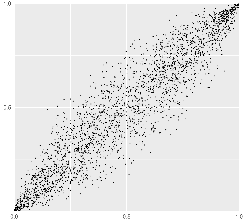
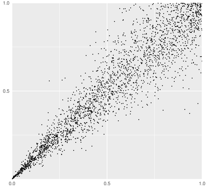
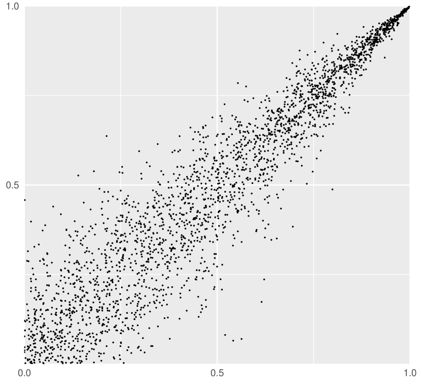
It remains to model the dependence structure of the hidden process To this end, we assume that the copulas between and are partially specified where we consider three different cases due to the following examples. In the first case, we consider Gaussian dependence specifications, in the second case Clayton copula specifications (which have lower tail dependencies), and in the third case survival Clayton copula specifications (which have upper tail dependencies). In each example, we determine sharp model uncertainty bounds for the distribution function of the maximum of the first observations. Figure 5 shows samples from the Gaussian, Clayton, and survival Clayton copula each having a parameter such that Kendall’s equals As we will see in the sequel, the tail dependencies have a strong effect on the distribution of the maximal observation, even under model uncertainty.
Example 4.2 (Gaussian dependencies in the hidden process)
We assume that the dependence structure of the hidden Markov process is partially specified by the Gaussian copulas
| (24) |
where the lower and upper correlation bounds are given by
for some small which serves as a dependence uncertainty parameter. For we are back in the setting of (20). Concerning the model uncertainty bounds, let and be hidden Markov processes specified by
| (25) | |||||||
| (26) | |||||||
where and are the systematic observation error bounds, see (22). It is well-known that the Gaussian copula family is -increasing in and that is CI for Further, the normal distribution is decreasing in with respect to the lower orthant order. Hence, using that the function in (18) is -antitone, we obtain from Corollary 4.1(b) for the distribution function of the maximal observations the following sharp model uncertainty bounds:
for all Figure 6 illustrates the uncertainty bands for the distribution function of , where the model uncertainty parameters are specified in the caption.
In the above example, we have modeled the dependencies in the hidden process with a Gaussian copula allowing slightly state-dependent increments of the random walk. In the following, we analyze the behaviour of the maximal observations when incorporating copula families with tail-dependencies into the hidden process. As an example, we consider Clayton and survival Clayton copulas specifying the dependencies of the hidden states where
| (27) |
denotes the Clayton and survival Clayton copula with parameter For the Clayton copula models independence and for it models comonotonicity. While Clayton copulas exhibit lower tail dependencies, their associated survival copulas have upper tail dependencies, see, e.g., [5] and Figure 5. To compare these models with the Gaussian dependence specifications, we consider Kendall’s as a measure that describes the degree of positive dependence between two random variables and we adjust the parameters accordingly for the Clayton and survival Clayton copulas. Hereby, Kendall’s of a Gaussian copula with parameter and Kendall’s of a Clayton copula with parameter are given by and see, e.g., [5, Table 6]. We use the transformation
| (28) |
to obtain the parameter of the Clayton copula as a function of the Gaussian copula parameter , so that both copulas exhibit the same degree of dependence in the sense of Kendall’s .
Example 4.3 (Clayton copula dependencies in the hidden process)
We now model the dependencies between the states of the hidden process with Clayton copulas, while leaving the marginal distributions, the dependencies between the hidden variables and the observations, and the dependence uncertainty parameters as before. More precisely, we consider a class of hidden Markov process which are partially specified by (22), (23), and with dependence uncertainty sets for the hidden process given by the transformations
| (29) |
where the lower and upper parameter bounds for the Clayton copulas are given by
Concerning the model uncertainty bounds, let and be hidden Markov processes with distributions uniquely specified by the marginal distributions in (25), the Gaussian copulas in (26) and the Clayton copulas
| (30) |
specifying the dependencies of the hidden process. Using that also the Clayton copula family is -increasing in and that is CI for we obtain, similar to Example 4.2, from Corollary 4.1(b) for the distribution function of the maximal observations the model uncertainty bounds
for all see Figure 6.
Example 4.4 (Survival Clayton copula dependencies in the hidden process)
To analyze the influence of tail dependencies, we now consider survival Clayton copulas as dependence specifications of the hidden process. The setting is similar to Example 4.3, but now (29) and (30) are replaced by
By definition of a survival copula, also the survival Clayton copula family in (27) is -increasing in and CI for Hence, similar as before, we obtain for the maximal observations the model uncertainty bounds
for all
Figure 6 illustrates the dependence uncertainty bands for the distribution function of the maximal observations in the classes of hidden Markov models considered in Examples 4.2 - 4.4. The dependence uncertainty parameters are chosen as i.e., the Pearson correlations in (20) and (21) are assumed to have some uncertainty and can vary up and down by . Setting we consider the maximum of the first observations. In the left plot, we illustrate the setting without systematic error, i.e., for all . In the right plot, we allow a systematic observation error between and for all As we see, the systematic errors directly affect the width of the uncertainty bands for the distribution function in the respective model. For comparison purposes, we include the distribution function of the maximum of the comonotonic observations , represented through the upper black line. The distribution of equals the distribution of for , where we set in the left figure and in the right figure. Additionally, we have plotted the distribution function of the maximum of an independent vector , represented through the lower black line, with zero mean in the left figure and mean in the right figure.
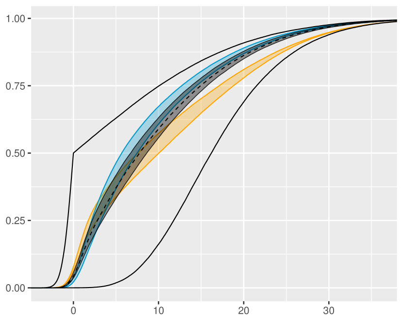
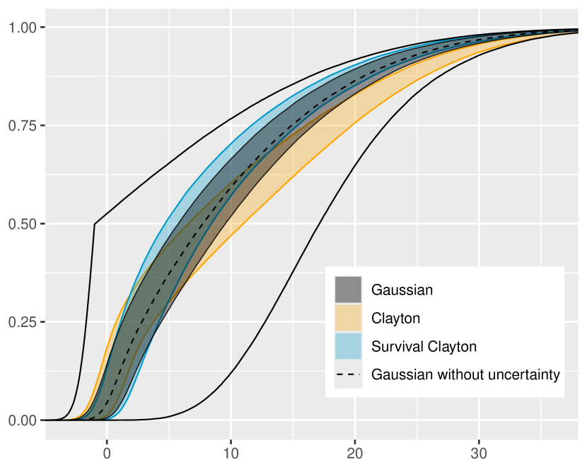
While the Gaussian copulas have no tail-dependence for the Clayton copulas exhibit lower tail-dependencies. In connection with this lower tail dependence, we observe that for small , the band is closer to the comonotonic distribution function compared to the case of the survival Clayton copula, which has upper tail dependence. However, this phenomenon reverses for large values of . In this case, the uncertainty band for the Clayton copula specifications is closer to the distribution function of the independent random variables. To analyze this behaviour in more detail, we write
| (31) | ||||
| (32) |
Due to Figure 6, the distribution function of the independent observations, denoted by , is pointwise smaller than the distribution function of the comonotonic observations This is a direct consequence of (12) but also very intuitive: It is more likely that in (31) is not greater than for all whenever are perfectly positive depend rather than independent. Similarly, we can explain the behaviour for the class of models where the hidden process has Clayton copula specifications: Due to lower tail-dependencies, for small the event tends to be more likely than in the Gaussian or survival Clayton copula case. Hence, the distribution function of the maximal observation is supposed to be larger and closer to comonotonicity. Vice versa, due to less positive dependence, for large the probability for some being larger than is higher compared to the other models, for which large observations occur more simultaneously. Hence, by (32), the distribution function of the maximum is supposed to be smaller in the Clayton copula model, which is confirmed by the plots. In contrast to the Clayton copula specifications, the class of hidden Markov models in Example 4.4 with survival Clayton copula specifications exhibits upper tail dependencies but no lower tail dependencies, see Figure 5. Hence, for large the probability that some exceeds is smaller and thus the distribution function of evaluated at is larger and closer to the comonotonic case. Further, for small the probability that all do not exceed is slightly smaller and closer to the independence case compared to the other models.
5 Discussion of the assumptions of Theorem 1.3
In this section, we discuss the generality of our main result, Theorem 1.3. First, we prove that none of the SI assumptions (i) and (ii) of Theorem 1.3 on and can be skipped or weakened to PSMD. Then, we show that a recently establish supermodular comparison result for star structures in [8], which allows to compare general dependencies with positive dependencies, cannot be extended to Markov processes and consequently also not to Markov tree distributions.
5.1 Discussion of the SI assumptions
Our main result, Theorem 1.3, provides simple conditions for a supermodular comparison of multivariate Markov tree distributions. At first glance, the SI conditions on and look rather unintuitive. However, as we show in the sequel, under ordering assumption (iii), they cannot be dropped or weakened. Figure 8 illustrates sufficient SI conditions in the three-dimensional case which, together with assumption (iii), leads to the supermodular comparison of Markov tree distributions. Whenever an SI condition in Theorem 1.3 is skipped, it implies the existence of subvectors exhibiting a dependence structure that aligns (or is even weaker) with SI conditions depicted by the graphs in Figure 8 a),b), or c). For these settings, we provide examples that do not imply a lower orthant comparison result and thus do not imply a supermodular comparison result neither. Proposition 5.2 summarizes the results of this section regarding the necessity of the SI conditions. In essence, for a Markov tree distribution on nodes, it is precisely these two SI conditions in Figure 8 c) that lead to a supermodular comparison result.
The following remark summarizes Examples A.3 – A.5 showing that the SI conditions in Figure 8 do not lead to comparison results as in Proposition 1.1 and Lemma 1.2.
Remark 5.1
- (a)
- (b)
- (c)
Using Examples A.3 – A.5 summarized in the preceding remark, we show in the following proposition that none of the SI conditions in assumptions (i) and (ii) of Theorem 1.3 can be dropped or weakened to PSMD. Since the supermodular order is closed under marginalization, see [104, Theorem 9.A.9(c)], the proof can be reduced to the cases considered above.
To this end, let be the tree, the path, and the specific child of the root as considered in Theorem 1.3. For a node that will be specified in Proposition 5.2, we relax the SI conditions in (i) and (ii) of Theorem 1.3 regarding only one edge: For let
| (33) | ||||
| (34) | ||||
| (35) |
Note that denotes the parent node of , see Definition B.1. We distinguish between three cases. The first one concerns the SI conditions on in (i). The second case relates to the SI conditions (ii) on , which states that for whenever , where is a nonempty set if and only if is not a star. In the third case we consider the SI conditions of the second part of (ii), which asserts that for , whenever , where is a nonempty set if and only if is not a chain. The following result states that none of the SI conditions in Theorem 1.3 can be dropped.
Proposition 5.2 (Generality of the SI assumptions of Theorem 1.3)
5.2 A special property of star structures
In this section, we discuss a considerable extension of the comparison results for star structures in Lemma 1.2 to a comparison of general dependencies, see [8]. The extension is based on the recently established Schur order for conditional distributions which compares conditional distribution functions of bivariate random vectors with respect to their strength of dependence in terms of their variability in the conditioning variable. The Schur order for conditional distributions has the fundamental properties that minimal elements characterize independence (i.e., no variability in the conditioning variable) and maximal elements characterize perfect dependence (i.e., maximal variability of the decreasing rearrangements), see [4, 5], where a random variable is said to completely or perfectly depend on if there exists a Borel measurable function (which is not necessarily increasing or decreasing) such that almost surely. Note that perfect dependence is not a symmetric concept, i.e., perfect dependence of on does not imply perfect dependence of on As we know from Lemma 1.2 on Markovian star structures, strong positive dependence between and for all leads to strong positive dependence among in the sense of the supermodular order. As it can easily be verified, also strong negative dependence between each and implies strong positive dependence among
A fairly intuitive result for Markovian star structures (Proposition 5.4) states that exhibits stronger positive dependence than whenever, for every is less dependent on the common factor variable than on in the sense of the Schur order for conditional distributions, where only is assumed to exhibit positive dependence. Similarly, one might expect for Markov chains that stronger dependence (in the sense of the Schur order) among than on for all would lead to stronger dependence among compared to , at least when all are conditionally increasing. Surprisingly, as we show below, comparison results with respect to the Schur order for conditional distributions cannot be extended from star structures to chain structures and thus neither to Markov tree distributions. In other words, only for star structures, more variability in the conditioning variable in the sense of the Schur order increases the strength of dependence of the whole vector in the supermodular order. Hence, Theorem 1.3 is also general in the sense that there is no extension to the Schur order for conditional distributions, which we formally define as follows, see [4].
Consider for integrable functions the Schur order defined by
| (36) | ||||
where denotes the decreasing rearrangement of an integrable function i.e., the essentially uniquely determined decreasing function such that for all where denotes the Lebesgue measure on see, e.g., [101]; for an overview of rearrangements, see [33, 34, 39, 55, 74, 97]. Roughly speaking, the decreasing rearrangement of a (piecewise constant) function can be obtained by rearranging the graph of the function in descending order. It is immediately clear that minimal elements in the Schur order are constant functions while maximal elements do in general not exist. The Schur order for conditional distributions is defined by comparing conditional distribution functions in their conditioning variable with respect to the Schur order for functions as defined in (36). We denote by the (generalized) quantile function of a random variable i.e.,
Definition 5.3 (Schur order for conditional distributions)
Let and be bivariate random vectors with Then the Schur order for conditional distributions is defined by
| (37) |
By definition, the Schur order for conditional distributions is invariant under rearrangements of the conditional variable and compares the variability of conditional distribution functions in the conditional variables in the sense of the Schur order for functions. Minimal elements characterize independence and maximal elements characterize complete directed dependence, see [4, Theorem 3.5]. Further, the Schur order for conditional distributions has the property that, for and
| (38) |
i.e., less variability of the conditional distribution function in the conditioning variable than in sense of (36) for all implies that is smaller or equal in the supermodular order than whenever is stochastically increasing in see [6, Proposition 3.17], cf. [4, Proposition 3.4]. Note that in (38), there is no positive dependence assumption on If additionally then also the reverse direction in (38) holds true, see [4, Proposition 3.4], cf. [6, 107]. In this case, the Schur order is equivalent to the supermodular order and we are back in the setting of Lemma 1.2.
The following result is a version of [8, Corollary 4(i)] and extends (38) to a vector of conditionally independent random variables. It states that a strengthening of the supermodular ordering condition to the Schur order allows to skip the positive dependence assumption (i) of Lemma 1.2 on
Proposition 5.4 (Comparison of star structure based on Schur order)
Let and be random vectors such that are conditionally independent given and such that are conditionally independent given with Assume for all that
-
(i)
-
(ii)
Then it follows that In particular, is positive supermodular dependent.
In the following remark, we discuss the special properties of star structures which allow a more general supermodular comparison result based on the Schur order for conditional distributions.
Remark 5.5
-
(a)
Since is equivalent to whenever and Proposition 5.4 extends Lemma 1.2 to a large class of conditionally independent distributions that allow a non-positive dependence structure of Surprisingly, as we show in Example A.6, Proposition 5.4 cannot be extended from star structures to Markov tree distributions: To be precise, let for and be a chain of nodes. Then, we can construct Markov tree distributed random variables and such that and is for all . Further, it holds that and for all as well as Hence, less variability of the bivariate specifications than with respect to the Schur order as in (37) does not imply that the entire vector is smaller than with respect to the lower orthant order and thus neither with respect to the supermodular order, even if the specifications satisfy the strong positive dependence concept see also Figure 8 d). Hence, Proposition 5.4 on the rearrangement-based Schur order is not extendable to Markov processes.
-
(b)
The Schur order for conditional distributions has the interesting property that it implies an ordering for various well-known dependence measures, where a dependence measure is a functional such that (i) (ii) if and only if and are independent, and (iii) if and only if is completely dependent on For example, Chatterjee’s rank correlation, which has recently attracted a lot of attention in the statistical literature [10, 30, 41], is consistent with the Schur order for conditional distributions [4]. Due to Proposition 5.4, the Schur order also implies general comparison results with respect to the supermodular order. Roughly speaking, large elements in the Schur order for conditional distributions lead to strong dependencies and, if the dependencies are positive, to large elements in supermodular order.
Acknowledgement
The first author gratefully acknowledges the support of the Austrian Science Fund (FWF) project P 36155-N ReDim: Quantifying Dependence via Dimension Reduction and the support of the WISS 2025 project ’IDA-lab Salzburg’ (20204-WISS/225/197-2019 and 20102-F1901166-KZP).
Appendix
Appendix A Examples
The following example justifies the assumption in Theorem 3.6 by showing that bivariate CI specifications do generally not lead to a Markov realization that is CI.
Example A.1 (A non-CI Markov tree distribution with bivariate CI marginals)
For consider the doubly stochastic matrices given by
Let be a random vector that follows a Markov tree distribution with respect to the tree , , , specified by the univariate and bivariate distributions through
| (39) | ||||
| (40) |
Note that the univariate distributions in (39) are the marginals of the bivariate distributions in (40). From the definition of the matrices and it can be seen that the subvectors and are CI . It even follows that is CI , because, as a consequence of Lemma B.3, and However, the vector is not CI because
is not increasing in Hence, if the bivariate specifications are CI, the implied Markov tree distribution is generally not CI.
The next example shows that Theorem 3.7 fails to hold when the continuity assumption on the marginal distribution functions is not imposed. In addition, the example emphasizes that the dependence structure of a random vector determined by a Markov realization of a bivariate tree specification is not only determined by the set of bivariate copulas and the conditional independence structure. It also depends on the choice of the marginal distributions.
Example A.2 (General marginals are not sufficient for Theorem 3.7)
Let be a tree with nodes and edges . Denote by the distribution function of the uniform distribution on Consider the marginal specifications and given by
Then and are continuous distribution functions and is the distribution function of the Dirac distribution in which is not continuous. Denote by the bivariate upper Fréchet copula, i.e., for and consider the bivariate specifications for Let and be independent and uniformly on distributed random variables. Then, for and the random vectors and are Markov realizations of and respectively, i.e.,
It holds that for all and (which trivially implies ) for Further, the bivariate copulas and are CI. Hence, all assumptions of Corollary 3.7i except of continuity of the marginal distributions are satisfied. However, it holds for all that
which implies
Since the lower orthant order is closed with respect to marginalization, see, e.g., [87, Theorem 3.3.19], it follows that .
Replacing in the above setting by and considering it follows similarly that and thus Hence, we conclude that the continuity assumption for the marginal specifications in Corollary 3.7 cannot be omitted.
Note that in this example, and are comonotonic while and are independent. Since the bivariate tree specifications and only differ in the first component of the marginal specifications (i.e., and ), we conclude that also the marginal distributions can affect the dependence structure of Markov tree distributions. In other words, conditional independence is not only a copula-dependent property.
The following example shows that the SI assumptions on and in opposite order in Proposition 1.1 cannot be replaced by SI in the same order, i.e., there is no version of Proposition 1.1 under the assumptions that and see also [45, Example 4.4]. We even show that, under two additional SI assumptions, see Figure 8 a) there is no supermodular comparison result.
Example A.3 (Condition (ii) in Proposition 1.1 cannot be replaced by )
Let , , , be a tree on nodes. Consider the doubly stochastic matrices given by
Let and be random vectors which follow a Markov tree distribution with respect to the tree specified by the bivariate distributions given by
All marginal distributions of the vectors and are uniform on i.e., for Further, for it holds that and thus, due to identical marginals, see (9). Moreover,
i.e., and are CIS, see Lemma B.3, and the bivariate subvectors and are CI. However, violates condition (ii) of Proposition 1.1 as well as condition (ii) of Theorem 1.3 since For the lower orthant set , we obtain
This shows that and thus, due to (8), . Hence, condition (ii) of Proposition 1.1 cannot be replaced by Similarly, this example highlights the importance of the assumption for all with in Theorem 1.3.
The following example shows that there is no version of Lemma 1.2 when assumptions (i) and (ii) are replaced by is CI and for . These SI conditions correspond to the graph in Figure 8 b).
Example A.4 (Conditions (i)-(ii) in Lemma 1.2 cannot be replaced by CI and )
Let be a tree on three nodes. Consider the doubly stochastic matrices defined by
| (41) | ||||
Let and be random vectors which follow a Markov tree distribution with respect to the tree specified by the bivariate distributions given by
All marginal distributions of the vectors and are uniform on i.e., for Further, for it holds that and thus, due to identical marginals, see (9). Moreover,
i.e., for the common factor variable is stochastically increasing and as well as are CI. For the lower orthant set , it holds that
| (42) |
This shows that and thus, due to (8), . Hence, condition (ii) of Lemma 1.2 cannot be replaced by Similarly, this example highlights the importance of the assumption for all with in Theorem 1.3.
The SI conditions in the following example correspond to the graph in Figure 8 c). This example is a comonotonic extension of Example A.4 and will also be used for the proof of Proposition 5.2 which provides the generality of the SI assumptions in Theorem 1.3.
Example A.5 (A commonotonic extension of Example A.4)
Let and be the random vectors in Example A.4. Define the ()-dimensional random vectors and by
Then and follow a Markov tree distribution with respect to the chain , where and . We have that
Moreover, it holds that for all . Using (42) we obtain for the lower orthant set that This shows that and thus . This example highlights the importance of the assumption for all with in Theorem 1.3 by extending the usage of Example A.4 to more complex cases, see also Proposition 5.2.
The following example shows that Proposition 5.4 based on the Schur order for conditional distributions cannot be extended to Markov processes and neither to Markov tree distributions.
Example A.6 (Schur order is not applicable to Markov processes)
Define the matrices by
| (43) |
Let and be random vectors which follow a Markov tree distribution with respect to the tree for and with bivariate distributions specified by
for all and All marginal distributions of the vectors and are uniform on i.e., for all It holds that is (thus, in particular, and , see (14)) and for all . Further, the bivariate distributions fulfill the Schur order criteria
| (44) |
i.e., for all edges and for all both has less variability than and has less variability than Since exhibits positive dependence (with respect to the strong notion ) one might expect that exhibits more positive dependence than and thus However, considering the lower orthant set , we obtain
which shows that and consequently . Note that Theorem 1.3 cannot be applied because so that the vector violates assumption (i).
Hence, the random vector is not smaller in supermodular order than even though, for all edges on the one hand has less variability and is closer to independence than with respect to the Schur order for conditional distributions, see (44). On the other hand, is PSMD and is i.e., all bivariate specifications exhibit positive dependencies.
To summarize, this example shows the importance of the SI assumptions in Theorem 1.3 on both and noting that the SI assumptions on cannot be skipped or weakened to PSMD even under the stronger comparison of the bivariate dependence specifications with respect to the Schur order for conditional distributions. This example also emphasises the special properties of star structures which allow a more general supermodular comparison result based on the Schur order for conditional distributions, see Proposition 5.4.
Appendix B Proofs of Section 1
In this section, we provide the proof of Theorem 1.3 which is based on combining Lemma 1.2 with an extension of the conditioning argument in [58, Theorem 3.2] to a non-stationary setting and to Markovian tree structures. For working with trees, this requires additional tools, which we introduce in the sequel. It is worth noting that Proposition 1.1 serves as an extension of [58, Theorem 3.2] to a non-stationary context. This proposition emerges as a direct consequence of Theorem 1.3.
In order to navigate through a tree, we define the commonly used notions of a parent, child, descendant, and ancestor relationship as follows.
Definition B.1 (Parent, child, descendant, ancestor, degree)
Let be a tree with root .
-
(i)
The parent of is defined as the unique element such that .
-
(ii)
The set of children of is defined by
-
(iii)
The set of descendants of is defined by
-
(iv)
The set of ancestors of is defined by
-
(v)
The degree of a node is defined by and .
According to its definition, a node is not included in the set of its children , descendants , or ancestors . Note that the root is the only element having no parent node.
The proof of Theorem 1.3 is based on an induction, which requires a specific enumeration of the nodes of the tree. To this end, we consider the level-order traversal where the nodes of the tree are visited level by level, starting from the root. This is also known as a breadth-first search. To be precise, we say that is an enumeration of if it is a one-to-one map from to . Further, is a level-order traversal if it is an enumeration such that for any pair of nodes and with (with respect to the order on ), the node is in a lower level of the tree compared to , i.e., for all
| (45) |
Note that this enumeration is not uniquely determined. We examplify the level order traversal in Figure 9 within a tree that comprises 8 nodes distributed across 3 levels.
To prove Theorem 1.3, we rely on several lemmas presented in the sequel. The subsequent lemma shows that if any random variable is SI in its ancestor random variables in a Markov tree distributed sequence, then any random vector corresponding to descendant nodes of this node is SI in the random variable associated to this current node. In the context of Markov processes, this means that if at each time step, the present random variable is SI in the preceding variable, then all future variables are SI in the present variable, see [45, Theorem 3.2]. We define, in comparison to Definition 2.1, the undirected paths
| (46) | ||||
Moreover, for a subset of nodes , we write and when referencing to the vector and random vector associated with these components.
Lemma B.2
Let be a sequence of random variables which follow a Markov tree distribution with respect to a tree . Assume that for all . Then, for all and for any finite subset , it follows that , i.e., for any increasing and bounded, the mapping
| (47) |
is increasing.
-
Proof:
We prove the result by induction over . Let , for . Then, by assumption, for all , see (46). We conclude by [45, Theorem 3.2] that . For the induction step, assume that the statement is valid for all such that . Suppose that has the form . The following part of the proof is divided in two cases. First, we assume that there are two nodes in which are not separated by , i.e.,
Then there is a node such that . In particular, the node can be choosen such that for all . Let be the last node in in the directed path from to , i.e.,
For we have for any increasing and bounded that
(48) where we use the Markov tree dependence for the second equality. Applying [45, Theorem 3.2] once more, we can conclude that is an increasing and bounded function in for all . Moreover, since is increasing, also the function is increasing in for all . Consequently, is increasing in each argument. By the induction hypothesis, we have that since and . Hence, by the definition of the stochastic order, the function in (48) is increasing in , proving that .
In the second case we assume that for all . For we have for any increasing and bounded that
| (49) |
by the Markov property. It follows that
| (50) | ||||
Since by assumption and, by the induction hypothesis, , we obtain that and the result is proven.
The following lemma, which we were unable to locate in the literature, shows that if all components , of a Markov tree distributed random vector in a random vector are SI in its parents, then is SI in all of its ancestors.
Lemma B.3
Let be a random vector that has Markov tree dependence with respect to a tree . If for all edges , then
| (51) |
-
Proof of Lemma B.3
In order to prove the statement, it is sufficient to prove that a Markov process is CIS if for all . For , the statement is trivial. By induction, we have to prove that is CIS if is CIS and . This follows if By the Markov property it holds that
(52) and the result is proven.
Note that property (51) is in general not a positive dependence concept unless follows a Markov tree distribution. For example, let , . For some independet and uniformly on distributed random variables and we define , , . Then meets (51), but is not positive lower (upper) orthant dependent, see Definition 2.8.
However, in the context of chains, property (51) is equivalent to the CIS property, and thus is a positive dependence concept in the sense of (14).
The following lemma extends [58, Theorem 3.1] from Markov processes to Markov tree distributions. It provides sufficient condition such that an integral of a supermodular function, under a conditional distribution, yields a supermodular function dependent on both the conditioning variable and the variables that remain unintegrated. Denote by the undirected path from to including and
Lemma B.4 (Supermodular conditional integration)
-
(i)
Let be a random vector that follows a Markov tree distribution with respect to a tree . Let and be a finite set. Assume that for all . Moreover let be an arbitrary finite index set and be a supermodular function on . Then the function given by
(53) is supermodular.
-
(ii)
The assumption for all in (i) can be weakened to for all edges of the subtree that consists of all paths from node to its descendants in
-
Proof:
(i) By the supermodularity of we obtain for , that the map
(54) is supermodular for all . In the following we show for that the map
(55) is supermodular for all . We fix . By the supermodularity of it follows for all that the map
(56) is increasing for all and . Similarly, the map
(57) is increasing for all and . By Lemma B.3 the assumption for all implies that for all . Thus, we can conclude from Lemma B.2 that . Now, for , we obtain that
(58) where the first inequality follows by and the increasingness of (56) for The second inequality holds true because the function in (57) is increasing. Now, (LABEL:eq:_lemma4_monotonicity) implies that
and we obtain the supermodularity of (55). Finally, the supermodularity in the cases (54) and (55) yields the supermodularity of (53), which proves the statement.
The following proposition is a version of Theorem 1.3 under additional SI assumptions. This result is used for the proof of Theorem 1.3 where we show that several SI conditions along a specified path can be omitted. We briefly outline the idea behind the proof of this proposition.
We initiate with the distribution of and replace the dependence specifications of for the specifications of iteratively over all star structures within the tree using a conditioning argument and applying Lemma 1.2 on the supermodular comparison of star structures. More precisely, for the induction, we navigate through the tree using a level-order traversal enumeration as described in (45). A disintegration argument allows us to reduce the proof of the statement in each step to the setting of Lemma 1.2. Finally, by the transitivity of the supermodular order, we obtain a supermodular comparison between and .
Proposition B.5
Let and be sequences of random variables that follow a Markov tree distribution with respect to a tree . Assume that
-
(i)
for all ,
-
(ii)
for all , and for all ,
-
(iii)
(resp. ) for all .
Then (resp. ).
-
Proof:
By the definitions of the stochastic orderings for stochastic processes (see Definition 2.7), we can assume that and . We only show the case that if for all . In the case where for all , it follows analogously that by reversing all inequality signs.
Denote by the vector of univariate marginal distribution functions of and . Note that for all because implies and Moreover, for , denote by and a copula for and , respectively, and define and . It follows that and , see Proposition 2.5. Let be a level-order traversal of as defined in (45). For , define the set of edges connecting the node with its children by . Then has a star-like structure. Note that if , then and thus . For , let be the set of bivariate copulas defined by(59) i.e., the specifications of the edges in the first stars in level-order traversal are replaced by the bivariate copula specifications of and the remaining edges are specified by the bivariate copulas associated to For consider the random vector . Note that and , which implies that and . We show that
(60) Then the statement follows from the transitivity of the supermodular order, see, e.g., [87]. In order to prove (60), fix . If we have that and thus which trivially implies . If , define and denote by an enumeration of the children of node Note that, by the definition of the bivariate copula sequences in (59), and can only differ in the copulas which correspond to the edges between node and its children, i.e., for all . For proving (60), it is sufficient to show for any bounded supermodular function that
(61) see [87, Theorem 3.9.14]. Recall that denotes the descendants of node see Definition B.1. Then we define the function on by
i.e., we integrate over all variables conditional on except of the variables associated to node and its descendants Then, we define recursively over the children of node for the functions by
i.e., the function is obtained through by integrating over the variables associated to all descendants of the ’th child of conditioned on the variable associated with . Finally, is a function in .
To prove supermodularity of , we will apply Lemma B.4. Recall that denotes the path from up to and including node . From the assumptions (ii) and (i) we know, in particular, that
| (62) | ||||
where, for a set the Cartesian product is denoted by Consider the subtree with nodes and edges . The nodes can be relabeled such that becomes the new root in . By (62) the Markov tree distributed sequence (with respect to the tree ) satisfies the assumptions of Lemma B.4 (ii) and by setting and (here still denotes the set of descendents of with respect to ) we obtain the supermodularity of .
To prove the supermodularity of , we assume by induction that is supermodular. By definition of and assumption we have that
| (63) |
Hence, we obtain supermodularity of by Lemma B.4 (ii) by setting and . and thus obtain the supermodularity of by Lemma B.4 (ii). In particular, we obtain that is supermodular.
Next, we show that
| (64) | ||||
| (65) |
From Markov tree dependence of and and since the sets of bivariate copulas and are identical for all edges , we have
| (66) | ||||
and
| (67) | ||||
for all . From (66), (67), and the disintegration theorem we obtain
| (68) | ||||
which shows (64). The proof for Equation (65) follows similarly replacing by in (68). Hence, we obtain from (64) and (65) that
For the second and third equality, we use that and which follows from the definition of and , respectively. For the inequality, we apply Lemma 1.2 using on the one hand that, by Markov tree dependence, the random variables are conditionally independent given and the random variables are conditionally independent given . On the other hand, by assumption (i), by assumption (ii), and for
This finally shows (61) and thus (60) for fixed . As we can repeat this procedure for each , the result is proven.
The comparison result formulated in Proposition B.5 is an extension of Lemma 1.2 to tree structures. However, it does not generalize Proposition 1.1 since the SI assumptions in Proposition B.5 are more stringent when applied to chains. It turns out that these SI assumptions on can be omitted in one direction along a specified path such that an generalization of Proposition 1.1 for trees can be formulated. This result is presented in Theorem 1.3 which can be proven by employing Proposition B.5 and an alternative adjustment of the dependencies, as described for the proof of Proposition B.5. As we show in the following proof of Theorem 1.3, we can omit the SI assumption on for one of the edges connected with the root and we can omit the SI assumptions on along a path through the tree starting with the root node and terminating at a leaf node whenever it has finite length. The proof of Theorem 1.3 is presented in the following.
-
Proof of Theorem 1.3
Similar to the proof of Proposition B.5, we can assume that . We show that . The proof for follows analogously. Denote by for the marginal distribution functions of and . Moreover, for , denote by and any copula for and , respectively, and define and . Then and , see Proposition 2.5. We enumerate the path such that for all , where and
In the following, we partition the tree along the nodes into disjoint subtrees, denoted as with corresponding disjoint sets of nodes and edges . As we will see, due to the selection of the subtrees, the subvectors and fulfill the assumptions of Proposition B.5 for all . We start with the definition of the set of nodes by
Recall that is due to the assumptions of Theorem 1.3 a child node of the root and lies in if and only if Note also that, for a node the set is defined as the set of descendants of Each set of nodes forms a tree along with its corresponding set of edges defined by
Note that some set of nodes may be empty or a singleton, depending on the structure of the tree . It holds that
i.e., is a partition of and is a partition of the set of edges without the edges that are contained in the specified path and without the edge between the root node and In the upcoming steps, we will sucessively replace the bivariate copulas of with those of . For , consider the sequences and of bivariate copulas given by
Furthermore, we define the sequence of bivariate copulas by
and for the sequences and of bivariate copulas by
Note that by definition . Keep in mind that our aim is to change all dependencies described by with the dependencies described by . The difference between the copula sets and lies in the replacement of the copula by . On the other hand, the difference between and is given by the replacement of the set of copulas by . Let
(69) (70) be random vectors on . The following part of the proof is divided into two steps. In the first step we show that and in the second step we show that .
Step 1: If , then which trivially implies For the other case, assume that We prove the supermodular comparison(71) To show the first inequality in (71), let be a bounded supermodular function. Since, by assumption (i), for all and for all , we can apply Lemma B.4(ii) twice and find that the function given by
(72) is supermodular. Note that we do not need any SI assumption on . By the the disintegration theorem and the Markov property, we have that
(73) where the last equality follows from Then the assumption together with (73) implies .
To show the second inequality in (71), again, let be a bounded supermodular function. Since, by assumption (i), for all and by assumption (ii), , we have that for all and . Due to Lemma B.2, we conclude that the function given by(74) is supermodular. By the disintegration theorem and the Markov property, we obtain
(75) where the second equality in the first and second line follow from and , respectively. Assumptions (i)- (iii), imply that the subvectors and fulfill the assumptions of Proposition B.5. Thus, (75) implies , which proves (71) using by the definition of and
Step 2: We aim to show that(76) The proof of (76) is devided into two parts. First, we show that
(77) and then show that
(78) To prove (77) let be a bounded and supermodular function and . If we have that and thus . So assume that Since, by assumption (ii), for all and if and for all we have that for all and if and for all . Further, by assumption (i), for all and consequently for all . Note that if and , it holds that , which belongs to the previous case. Now, we obtain from Lemma B.4 (ii), applied on the subtree with nodes and root by setting and , that the function given by
(79) is supermodular. Then we obtain
(80) where the first equality in each line follows by the disintegration theorem and the Markov property and the second ones since and by definition of and in (70). Assumptions (i)- (iii) of Theorem 1.3, imply that the subvectors and fulfill the assumptions of Proposition B.5 which implies . Together with (80), we obtain (77).
To prove (78), let again be a bounded and supermodular function and . Since, by assumption (ii), for all and if and for all , we have that for all and if and for all . Further, by assumption (i), for all and consequently for all . We apply Lemma B.4 (ii) twice and find that the function given by
(81) is supermodular. Again, we obtain
(82) By assumption (iii) it holds that , which together with (82) implies (78).
By (77) and (78) we conclude (76). Finally, , (76) and the transitivity of the supermodular order imply that , which proves the first statement.
To show positive supermodular dependence of , we apply the first statement on and . Note that the random vector fulfills assumption (ii) trivially. Since fulfills assumption (i), we have for that which implies , see (14). Hence, with the additional assumption of positive supermodular dependence of , we obtain for all i.e., assumption (iii) holds for all . From the first part, we now conclude that .
A similar argument yields positive supermodular dependence of under assumption (ii) and positive supermodular dependence of for
Appendix C Proofs of Section 2
-
Proof of Proposition 2.5
For , we prove the statement by an induction over the number of nodes . Starting with , the statement is trivial. For the induction step, assume that the statement is true for each tree with nodes for a fixed We need to show the statement for . By re-enumeration we may assume that the node is a leaf in with parent node , i.e., and , see Definition B.1. We define the subtree with nodes and edges , which is a tree with nodes. By the induction hypothesis, there is a Markov tree distribution specified through . Let be a bivariate random vector having distribution function defined through Sklar’s theorem. For Borel sets , we define the distribution on by
(83) Similar to the proof of [80, Theorem 2], it follows that is the unique distribution with the given specifications that has Markov tree dependence. For , the distribution can be obtained by the Kolmogorov extension Theorem, see [66, Theorem 6.16], where the assumption of projective families is satisfied as a consequence of the disintegration theorem.
Appendix D Proofs of Section 3
For a random vector with distribution function , we denote by the survival function of which is given by
There is also an analogous version of Sklar’s Theorem for survival functions, cf. [42, Theorem 2.2.13], which states that for any survival function with survival marginals , , there is a copula , such that
| (84) |
The copula is called survival copula of . The following lemma shows that the copula (survival copula) of a Markov tree distribution with respect to a tree , specified by continuous marginal distribution functions and bivariate copulas , is given by the distribution function (the survival copula) of the Markov tree distribution specified by uniform marginals on and the bivariate copulas . This is especially useful for comparing bivariate tree specification with the same bivariate copula structure but different marginal distributions.
Lemma D.1
Let be a random vector with continuous marginal specifications . Moreover, let be a random vector with distribution function , where denotes the distribution function of the uniform distribution on . Then the following hold true:
-
(i)
is the unique copula for , i.e., .
-
(ii)
The survival function and the survival copula of are related by
(85) Further is the unique survival copula of , i.e., is the unique copula such that
(86) where is the survival function of
-
Proof of Lemma D.1
We prove statement (i) by an induction over the number of nodes . Starting with , the statement is trivial. For the induction step, assume that the statement is true for each tree with nodes for a fixed We need to show the statement for . By re-enumeration we may assume that is a leaf in with parent node , i.e., and , see Definition B.1. We define the subtree with nodes and edges which is a tree with number of nodes . By (83) and the transformation formula, using that -a.s., cf. [101, Theorem 1.2], we have that
(87) Since the marginal distribution functions are continuous, the distribution function of the transformed random vector is the unique copula of , see, e.g., [99, Remark 2.2]. Moreover, by the induction hypothesis the distribution function is also a copula for . By uniqueness of the copula, we obtain that . By [6, Theorem 2.2], we have
where denotes the operator that takes the partial derivative with respect to the first component. Hence, we obtain that (87) equals
which proves the first result. We continue with statement (ii). Equation (85) follows directly by
(88) By [42, Theorem 2.2.13] and the continuity of the survival copula for is unique and it remains to show equation (86). By the inclusion-exclusion principle we obtain that
-
Proof of Theorem 3.6
By the definition of the orders for stochastic processes, Definition 2.7 (b), we may assume that . Let be a random vector having the same marginals as and the same bivariate dependence specifications as By assumption (ii) and (14) the copulas , are CI and thus is CI for all . We deduce from Theorem 1.3 that and consequently . When verifying the assumptions for Theorem 1.3, it is worth noting that distinguishing between the cases where and is not necessary since is CI for all and consequently in the case where , it is always possible to select the path in the assumptions of Theorem 1.3 in such a way that According to [44, Proposition 7.1], the vectors and are MTP2 and thus CI. By the continuity of and for all and Lemma D.1, the vectors and have the same copula which is CI. Hence, we obtain from [85, Theorem 4.5] using that for all , that . The transitivity of the directionally convex order implies .
-
Proof of Theorem 3.7
Consider a sequence of Markov tree distributed random variables. Since fulfills assumption (ii) of Theorem 1.3 this is also the case for . Moreover and have the same marginal distributions. Hence, and fulfill the assumptions of Theorem 1.3 and we obtain that . Due to (8), it holds that and . By the transitivity of the lower and upper orthant order it remains to show that (resp. ). Since the marginal distribution functions and are assumed to be continuous and since and have the same bivariate specifications, Lemma D.1 (i) implies that and have the same copula . Since, by assumption, for all we obtain from Sklar’s Theorem that
for all This proves To show let be the common survival copula of and , see Lemma D.1 (ii). Since, by assumption, for all we obtain
for all which concludes the proof.
Appendix E Proofs of Section 4
- Proof of Corollary 4.1
Appendix F Proofs of Section 5
- Proof of Proposition 5.2
(a) For the first statement, we consider two cases. If , i.e., is an element of the decedents of , we define the vectors by and , where and are given by Example A.5. Then we extend these vectors by independent random variables (note that the independence copula is CI) to the Markov tree distributed sequences and . These vectors fulfill assumption () in (33), and the assumptions (ii) and (iii) of Theorem 1.3. Since , we obtain from the closure of the lower orthant order under marginalization that and thus In the case where , which implies , we define the vectors and , and proceed as in the first case.
(b) Since is not a star it holds . The node has a parent node and has at least one child node . Define the subvectors and as in Example A.3 and extend these -dimensional vectors by independent random variables (note that the independence copula is CI) to the random vectors and . Then and fulfill assumption () in (34), and the assumptions (i) and (iii) of Theorem 1.3. We obtain from Example A.3 that and thus and . This shows the second statement.
(c) Since is not a chain, we have . For we consider the directed path from the root to . Let be the last node in such that , i.e., the unique node such that . Since and the node has a child node . Define the subvectors and as in Example A.5 and extend this -dimensional vectors by independent random variables (note that the independence copula is CI) to the random vectors and . Then and fulfill assumption () in (35), and the assumptions (i) and (iii) of Theorem 1.3. Due to Example A.5, we obtain and consequently and . This shows the third statement and the result is proven.
References
- Abdous et al. [2005] B. Abdous, C. Genest, and B. Rémillard. Dependence properties of meta-elliptical distributions. In Statistical modeling and analysis for complex data problems, pages 1–15. Springer, 2005.
- Acar et al. [2012] E. F. Acar, C. Genest, and J. Neslehová. Beyond simplified pair-copula constructions. J. Multivariate Anal., 110:74–90, 2012.
- Akaike [1974] H. Akaike. Markovian representation of stochastic processes and its application to the analysis of autoregressive moving average processes. Ann. Inst. Stat. Math., 26:363–387, 1974.
- Ansari and Fuchs [2022] J. Ansari and S. Fuchs. A simple extension of azadkia and chatterjee’s rank correlation to a vector of endogenous variables. arXiv preprint arXiv:2212.01621, 2022.
- Ansari and Rockel [2024] J. Ansari and M. Rockel. Dependence properties of bivariate copula families. Accepted for publication in: Depend. Model., 2024.
- Ansari and Rüschendorf [2021] J. Ansari and L. Rüschendorf. Sklar’s theorem, copula products, and ordering results in factor models. Depend. Model., 9:267–306, 2021.
- Ansari and Rüschendorf [2021] J. Ansari and L. Rüschendorf. Ordering results for elliptical distributions with applications to risk bounds. J. Multivariate Anal., 182:14, 2021.
- Ansari and Rüschendorf [2024] J. Ansari and L. Rüschendorf. Supermodular and directionally convex comparison results for general factor models. J. Multivariate Anal., 201:20, 2024. Id/No 105264.
- Ansari et al. [2024] J. Ansari, E. Lütkebohmert, A. Neufeld, and J. Sester. Improved robust price bounds for multi-asset derivatives under market-implied dependence information. Accepted for publication in: Finance Stoch., 2024.
- Azadkia and Chatterjee [2021] M. Azadkia and S. Chatterjee. A simple measure of conditional dependence. Ann. Stat., 49(6):3070–3102, 2021.
- Backhoff et al. [2017] J. Backhoff, M. Beiglböck, Y. Lin, and A. Zalashko. Causal transport in discrete time and applications. SIAM J. Optim., 27(4):2528–2562, 2017.
- Backhoff Veraguas et al. [2020] J. Backhoff Veraguas, M. Beiglböck, M. Eder, and A. Pichler. Fundamental properties of process distances. Stochastic Processes Appl., 130(9):5575–5591, 2020.
- Bartl et al. [2021] D. Bartl, M. Beiglböck, and G. Pammer. The wasserstein space of stochastic processes. arXiv preprint arXiv:2104.14245, 2021.
- Bäuerle [1997] N. Bäuerle. Inequalities for stochastic models via supermodular orderings. Commun. Stat., Stochastic Models, 13(1):181–201, 1997.
- Bäuerle and Müller [2006] N. Bäuerle and A. Müller. Stochastic orders and risk measures: consistency and bounds. Insur. Math. Econ., 38(1):132–148, 2006.
- Bäuerle and Rolski [1998] N. Bäuerle and T. Rolski. A monotonicity result for the workload in Markov-modulated queues. J. Appl. Probab., 35(3):741–747, 1998.
- Bedford and Cooke [2002] T. Bedford and R. M. Cooke. Vines – a new graphical model for dependent random variables. Ann. Stat., 30(4):1031–1068, 2002.
- Beiglböck and Juillet [2016] M. Beiglböck and N. Juillet. On a problem of optimal transport under marginal martingale constraints. Ann. Probab., 44(1):42–106, 2016.
- Beiglböck et al. [2013] M. Beiglböck, P. Henry-Labordère, and F. Penkner. Model-independent bounds for option prices – a mass transport approach. Finance Stoch., 17(3):477–501, 2013.
- Beiglböck et al. [2017] M. Beiglböck, M. Nutz, and N. Touzi. Complete duality for martingale optimal transport on the line. Ann. Probab., 45(5):3038–3074, 2017.
- Belzunce et al. [2009] F. Belzunce, J.-A. Mercader, J.-M. Ruiz, and F. Spizzichino. Stochastic comparisons of multivariate mixture models. J. Multivariate Anal., 100(8):1657–1669, 2009.
- Benjamini and Peres [1994] I. Benjamini and Y. Peres. Markov chains indexed by trees. Ann. Probab., 22(1):219–243, 1994.
- Bernard et al. [2017] C. Bernard, L. Rüschendorf, S. Vanduffel, and R. Wang. Risk bounds for factor models. Finance Stoch., 21(3):631–659, 2017.
- Biller and Corlu [2011] B. Biller and C. G. Corlu. Accounting for parameter uncertainty in large-scale stochastic simulations with correlated inputs. Operations Research, 59(3):661–673, 2011.
- Block and Sampson [1988] H. W. Block and A. R. Sampson. Conditionally ordered distributions. J. Multivariate Anal., 27(1):91–104, 1988.
- Brechmann et al. [2012] E. C. Brechmann, C. Czado, and K. Aas. Truncated regular vines in high dimensions with application to financial data. Can. J. Stat., 40(1):68–85, 2012.
- Breeden and Litzenberger [1978] D. T. Breeden and R. H. Litzenberger. Prices of state-contingent claims implicit in option prices. Journal of business, pages 621–651, 1978.
- Burgert and Rüschendorf [2006] C. Burgert and L. Rüschendorf. Consistent risk measures for portfolio vectors. Insur. Math. Econ., 38(2):289–297, 2006.
- Cappé et al. [2005] O. Cappé, E. Moulines, and T. Rydén. Inference in hidden markov models. Springer New York, NY, 2005.
- Chatterjee [2021] S. Chatterjee. A new coefficient of correlation. J. Am. Stat. Assoc., 116(536):2009–2022, 2021.
- Chatterjee and Vidyasagar [2022] S. Chatterjee and M. Vidyasagar. Estimating large causal polytree skeletons from small samples. arXiv preprint arXiv:2209.07028, 2022.
- Chevallier et al. [2019] J. Chevallier, D. K. Nguyen, and J. C. Reboredo. A conditional dependence approach to co2-energy price relationships. Energy Economics, 81:812–821, 2019.
- Chong [1974] K.-M. Chong. Some extensions of a theorem of Hardy, Littlewood and Polya and their applications. Can. J. Math., 26:1321–1340, 1974.
- Chong and Rice [1971] K. M. Chong and N. M. Rice. Equimeasurable Rearrangements of Functions. Queen’s University, Kingston, Ontario, 1971.
- Cooke [1997] R. M. Cooke. Markov and entropy properties of tree-and vine-dependent variables. In Proceedings of the ASA section of Bayesian statistical science, volume 27, 1997.
- Czado [2019] C. Czado. Analyzing dependent data with vine copulas. A practical guide with R, volume 222 of Lect. Notes Stat. Cham: Springer, 2019.
- Czado and Nagler [2022] C. Czado and T. Nagler. Vine copula based modeling. Annual Review of Statistics and Its Application, 9:453–477, 2022.
- Daduna and Szekli [2006] H. Daduna and R. Szekli. Dependence ordering for Markov processes on partially ordered spaces. J. Appl. Probab., 43(3):793–814, 2006.
- Day [1972] P. W. Day. Rearrangement inequalities. Can. J. Math., 24:930–943, 1972.
- Derumigny and Fermanian [2017] A. Derumigny and J.-D. Fermanian. About tests of the “simplifying” assumption for conditional copulas. Depend. Model., 5:154–197, 2017.
- Dette et al. [2013] H. Dette, K. F. Siburg, and P. A. Stoimenov. A copula-based non-parametric measure of regression dependence. Scand. J. Stat., 40(1):21–41, 2013.
- Durante and Sempi [2016] F. Durante and C. Sempi. Principles of copula theory. Boca Raton, FL: CRC Press, 2016.
- Ephraim and Merhav [2002] Y. Ephraim and N. Merhav. Hidden markov processes. IEEE Transactions on information theory, 48(6):1518–1569, 2002.
- Fallat et al. [2017] S. Fallat, S. Lauritzen, K. Sadeghi, C. Uhler, N. Wermuth, and P. Zwiernik. Total positivity in Markov structures. Ann. Stat., 45(3):1152–1184, 2017.
- Fang et al. [1994] Z. Fang, T. Hu, and H. Joe. On the decrease in dependence with lag for stationary markov chains. Probability in the Engineering and Informational Sciences, 8(3):385–401, 1994.
- Farrokhi et al. [2021] A. Farrokhi, S. Farzin, and S.-F. Mousavi. Meteorological drought analysis in response to climate change conditions, based on combined four-dimensional vine copulas and data mining (vc-dm). Journal of Hydrology, 603:127135, 2021.
- Föllmer and Schied [2016] H. Föllmer and A. Schied. Stochastic Finance. An Introduction in Discrete Time. De Gruyter Textb. Berlin: de Gruyter, 4th revised edition edition, 2016.
- Garralda Guillem [2000] A. I. Garralda Guillem. Structure of dependence for bivariate extreme value distributions. C. R. Acad. Sci., Paris, Sér. I, Math., 330(7):593–596, 2000.
- Genon-Catalot et al. [2000] V. Genon-Catalot, T. Jeantheau, and C. Larédo. Stochastic volatility models as hidden Markov models and statistical applications. Bernoulli, 6(6):1051–1079, 2000.
- Ghoussoub et al. [2019] N. Ghoussoub, Y.-H. Kim, and T. Lim. Structure of optimal martingale transport plans in general dimensions. Ann. Probab., 47(1):109–164, 2019.
- Gijbels et al. [2017] I. Gijbels, M. Omelka, and N. Veraverbeke. Nonparametric testing for no covariate effects in conditional copulas. Statistics, 51(3):475–509, 2017.
- Gill et al. [2011] S. Gill, B. Stephen, and S. Galloway. Wind turbine condition assessment through power curve copula modeling. IEEE Transactions on Sustainable Energy, 3(1):94–101, 2011.
- Gunasingam and Wong [2024] M. Gunasingam and T.-K. L. Wong. Adapted optimal transport between gaussian processes in discrete time. arXiv preprint arXiv:2404.06625, 2024.
- Hamilton [1989] J. D. Hamilton. A new approach to the economic analysis of nonstationary time series and the business cycle. Econometrica: Journal of the econometric society, pages 357–384, 1989.
- Hardy et al. [1929] G. H. Hardy, J. E. Littlewood, and G. Pólya. Some simple inequalities satisfied by convex functions. Messenger 58, 145-152 (1929)., 1929.
- Hofert and Pham [2013] M. Hofert and D. Pham. Densities of nested Archimedean copulas. J. Multivariate Anal., 118:37–52, 2013.
- Hu and Joe [1995] T. Hu and H. Joe. Monotonicity of positive dependence with time for stationary reversible Markov chains. Probab. Eng. Inf. Sci., 9(2):227–237, 1995.
- Hu and Pan [2000] T. Hu and X. Pan. Comparisons of dependence for stationary Markov processes. Probab. Eng. Inf. Sci., 14(3):299–315, 2000.
- Jaworski et al. [2013] P. Jaworski, F. Durante, and W. K. Härdle, editors. Copulae in mathematical and quantitative finance. Proceedings of the workshop, Cracow, Poland, July 10–11, 2012, volume 213 of Lect. Notes Stat. Berlin: Springer, 2013.
- Jiao and Emura [2023] Z. Jiao and K. Emura. Estimation of outdoor design dataset based on interdependency of multiple meteorological elements by using vine copulas. Energy and Buildings, 280:112724, 2023.
- Joe [1990] H. Joe. Multivariate concordance. J. Multivariate Anal., 35(1):12–30, 1990.
- Joe [1997] H. Joe. Multivariate models and dependence concepts, volume 73 of Monogr. Stat. Appl. Probab. London: Chapman and Hall, 1997.
- Joe and Kurowicka [2011] H. Joe and D. Kurowicka. Dependence Modeling: Vine Copula Handbook. World Scientific, 2011.
- Jouini et al. [2006] E. Jouini, W. Schachermayer, and N. Touzi. Law invariant risk measures have the Fatou property. In Adv. Math. Econ. Vol. 9, pages 49–71. Tokyo: Springer, 2006.
- Kailath and Poor [1998] T. Kailath and H. V. Poor. Detection of stochastic processes. IEEE Transactions on Information Theory, 44(6):2230–2231, 1998.
- Kallenberg [2021] O. Kallenberg. Foundations of modern probability. In 2 volumes, volume 99 of Probab. Theory Stoch. Model. Cham: Springer, 3rd revised and expanded edition edition, 2021.
- Kirshner [2007] S. Kirshner. Learning with tree-averaged densities and distributions. Advances in Neural Information Processing Systems, 20, 2007.
- Koller and Friedman [2009] D. Koller and N. Friedman. Probabilistic graphical models. Adapt. Comput. Mach. Learn. Cambridge, MA: MIT Press, 2009.
- Kulik and Szekli [2001] R. Kulik and R. Szekli. Sufficient conditions for long-range count dependence of stationary point processes on the real line. J. Appl. Probab., 38(2):570–581, 2001.
- Langrock et al. [2012] R. Langrock, I. L. MacDonald, and W. Zucchini. Some nonstandard stochastic volatility models and their estimation using structured hidden markov models. Journal of Empirical Finance, 19(1):147–161, 2012.
- Lin et al. [2020] Y. Lin, Y. Xiao, and F. Li. Forecasting crude oil price volatility via a hm-egarch model. Energy Economics, 87:104693, 2020.
- Lopez-Paz et al. [2013] D. Lopez-Paz, J. M. Hernández-Lobato, and G. Zoubin. Gaussian process vine copulas for multivariate dependence. In International Conference on Machine Learning, pages 10–18. PMLR, 2013.
- Lux and Papapantoleon [2017] T. Lux and A. Papapantoleon. Improved Fréchet-Hoeffding bounds on -copulas and applications in model-free finance. Ann. Appl. Probab., 27(6):3633–3671, 2017.
- Luxemburg [1967] W. A. J. Luxemburg. Rearrangement invariant Banach function spaces. Proc. Symp. Analysis, Queen’s Univ. 1967, Queen’s Pap. Pure Appl. Math. 10, 83-144 (1967)., 1967.
- Mamon and Elliott [2007] R. S. Mamon and R. J. Elliott, editors. Hidden Markov Models in Finance, volume 104 of Int. Ser. Oper. Res. Manag. Sci. New York, NY: Springer, 2007.
- Marshall et al. [2011] A. W. Marshall, I. Olkin, and B. C. Arnold. Inequalities: theory of majorization and its applications. Springer Ser. Stat. New York, NY: Springer, 2nd edition edition, 2011.
- McNeil [2008] A. J. McNeil. Sampling nested Archimedean copulas. J. Stat. Comput. Simulation, 78(5-6):567–581, 2008.
- McNeil and Neslehová [2009] A. J. McNeil and J. Neslehová. Multivariate Archimedean copulas, -monotone functions and -norm symmetric distributions. Ann. Stat., 37(5B):3059–3097, 2009.
- McNeil et al. [2015] A. J. McNeil, R. Frey, and P. Embrechts. Quantitative Risk Management. Concepts, Techniques and Tools. Princeton, NJ: Princeton University Press, revised edition edition, 2015.
- Meeuwissen and Cooke [1994] A. M. H. Meeuwissen and R. M. Cooke. Tree dependent random variables. Delft University of Technology, Faculty of Technical Mathematics and Informatics, 1994.
- Mroz et al. [2021] T. Mroz, S. Fuchs, and W. Trutschnig. How simplifying and flexible is the simplifying assumption in pair-copula constructions – analytic answers in dimension three and a glimpse beyond. Electron. J. Stat., 15(1):1951–1992, 2021.
- Müller [2001] A. Müller. Stochastic ordering of multivariate normal distributions. Ann. Inst. Stat. Math., 53(3):567–575, 2001.
- Müller [2013] A. Müller. Duality theory and transfers for stochastic order relations. In Stochastic orders in reliability and risk, Xiamen, China, June 27–29, 2011. New York, NY: Springer, 2013.
- Müller and Scarsini [2000] A. Müller and M. Scarsini. Some remarks on the supermodular order. J. Multivariate Anal., 73(1):107–119, 2000.
- Müller and Scarsini [2001] A. Müller and M. Scarsini. Stochastic comparison of random vectors with a common copula. Math. Oper. Res., 26(4):723–740, 2001.
- Müller and Scarsini [2005] A. Müller and M. Scarsini. Archimedean copulae and positive dependence. J. Multivariate Anal., 93(2):434–445, 2005.
- Müller and Stoyan [2002] A. Müller and D. Stoyan. Comparison methods for stochastic models and risks. Wiley Ser. Probab. Stat. Chichester: Wiley, 2002.
- Nelsen [2006] R. B. Nelsen. An introduction to copulas. 2nd ed. New York, NY: Springer, 2006.
- Pemantle [1995] R. Pemantle. Tree-indexed processes. Stat. Sci., 10(2):200–213, 1995.
- Pu and Yin [2021] T. Pu and C. Yin. Stochastic orderings of the location-scale mixture of elliptical distribution. arXiv preprint arXiv:2103.16227, 2021.
- Pu et al. [2023] T. Pu, Y. Zhang, and C. Yin. Generalized location-scale mixtures of elliptical distributions: Definitions and stochastic comparisons. Communications in Statistics-Theory and Methods, pages 1–25, 2023.
- Rachev and Rüschendorf [1998] S. T. Rachev and L. Rüschendorf. Mass transportation problems. Vol. 1: Theory. Vol. 2: Applications. Springer Ser. Stat. New York, NY: Springer, 1998.
- Rebane and Pearl [2013] G. Rebane and J. Pearl. The recovery of causal poly-trees from statistical data. arXiv preprint arXiv:1304.2736, 2013.
- Rossi and Gallo [2006] A. Rossi and G. M. Gallo. Volatility estimation via hidden markov models. Journal of Empirical Finance, 13(2):203–230, 2006.
- Rüschendorf [1980] L. Rüschendorf. Inequalities for the expectation of -monotone functions. Z. Wahrscheinlichkeitstheor. Verw. Geb., 54:341–349, 1980.
- Rüschendorf [1981a] L. Rüschendorf. Characterization of dependence concepts in normal distributions. Ann. Inst. Stat. Math., 33:347–359, 1981a.
- Rüschendorf [1981b] L. Rüschendorf. Ordering of distributions and rearrangement of functions. Ann. Probab., 9:276–283, 1981b.
- Rüschendorf [1985] L. Rüschendorf. The Wasserstein distance and approximation theorems. Z. Wahrscheinlichkeitstheor. Verw. Geb., 70:117–129, 1985.
- Rüschendorf [2005] L. Rüschendorf. Stochastic ordering of risks, influence of dependence and a.s. constructions. Advances on Models, Characterizations and Applications, pages 19–56, 2005.
- Rüschendorf [2012] L. Rüschendorf. Worst case portfolio vectors and diversification effects. Finance Stoch., 16(1):155–175, 2012.
- Rüschendorf [2013] L. Rüschendorf. Mathematical Risk Analysis. Dependence, Risk Bounds, Optimal Allocations and Portfolios. Springer Ser. Oper. Res. Financ. Eng. Berlin: Springer, 2013.
- Rüschendorf [2017] L. Rüschendorf. Risk bounds and partial dependence information. In From Statistics to Mathematical Finance. Festschrift in honour of Winfried Stute, pages 345–366. Cham: Springer, 2017.
- Rüschendorf et al. [2016] L. Rüschendorf, A. Schnurr, and V. Wolf. Comparison of time-inhomogeneous Markov processes. Adv. Appl. Probab., 48(4):1015–1044, 2016.
- Shaked and Shantikumar [2007] M. Shaked and J. G. Shantikumar. Stochastic Orders. Springer Ser. Stat. New York, NY: Springer, 2007.
- Shaked and Tong [1985] M. Shaked and Y. L. Tong. Some partial orderings of exchangeable random variables by positive dependence. J. Multivariate Anal., 17:333–349, 1985.
- Slepian [1962] D. Slepian. The one-sided barrier problem for gaussian noise. Bell System Technical Journal, 41(2):463–501, 1962.
- Strothmann et al. [2024] C. Strothmann, H. Dette, and K. F. Siburg. Rearranged dependence measures. Bernoulli, 30(2):1055–1078, 2024.
- Sun et al. [2018] M. Sun, I. Konstantelos, and G. Strbac. A deep learning-based feature extraction framework for system security assessment. IEEE transactions on smart grid, 10(5):5007–5020, 2018.
- Talponen and Viitasaari [2014] J. Talponen and L. Viitasaari. Note on multidimensional Breeden-Litzenberger representation for state price densities. Math. Financ. Econ., 8(2):153–157, 2014.
- Tankov [2011] P. Tankov. Improved Fréchet bounds and model-free pricing of multi-asset options. J. Appl. Probab., 48(2):389–403, 2011.
- Tchen [1980] A. H. Tchen. Inequalities for distributions with given marginals. Ann. Probab., 8:814–827, 1980.
- Tong [1977] Y. L. Tong. An ordering theorem for conditionally independent and identically distributed random variables. Ann. Stat., 5:274–277, 1977.
- Tong [1980] Y. L. Tong. Probability inequalities in multivariate distributions. Probability and Mathematical Statistics. New York etc.: Academic Press (A Subsidiary of Harcourt Brace Jovanovich, Publishers). XIII, p. 239, 1980.
- Tong [1989] Y. L. Tong. Inequalities for a class of positively dependent random variables with a common marginal. Ann. Stat., 17(1):429–435, 1989.
- Villani [2009] C. Villani. Optimal transport. Old and new, volume 338 of Grundlehren Math. Wiss. Berlin: Springer, 2009.
- Wang et al. [2017] Z. Wang, W. Wang, C. Liu, Z. Wang, and Y. Hou. Probabilistic forecast for multiple wind farms based on regular vine copulas. IEEE Transactions on Power Systems, 33(1):578–589, 2017.
- Weiß and Supper [2013] G. N. Weiß and H. Supper. Forecasting liquidity-adjusted intraday value-at-risk with vine copulas. Journal of Banking & Finance, 37(9):3334–3350, 2013.
- Wuertz et al. [2013] D. Wuertz, S. RUnit, and M. Y. Chalabi. Package ‘fgarch’. Technical report, Technical report, working paper/manual, 09.11.2009., 2013.
- Xiong et al. [2014] L. Xiong, K.-x. Yu, and L. Gottschalk. Estimation of the distribution of annual runoff from climatic variables using copulas. Water Resources Research, 50(9):7134–7152, 2014.
- Yin [2021] C. Yin. Stochastic orderings of multivariate elliptical distributions. J. Appl. Probab., 58(2):551–568, 2021.
- Zaev [2015] D. A. Zaev. On the Monge-Kantorovich problem with additional linear constraints. Math. Notes, 98(5):725–741, 2015.