Bayesian synthesis of astrometric wobble and total light curves in
close binary supermassive black holes
Abstract
We test the potential of Bayesian synthesis of upcoming multi-instrument data to extract orbital parameters and individual light curves of close binary supermassive black holes (CB-SMBH) with subparsec separations. Next generation (ng) interferometers, will make possible the observation of astrometric wobbles in CB-SMBH. Combining them with periodic variable time-domain data from surveys like the Vera C. Rubin Legacy Survey of Space and Time (LSST), allows for a more information on CB-SMBH candidates compared to standalone observational methods. Our method reliably determines binary parameters and component fluxes from binary total flux across long-term, intermediate and short-term binary dynamics and observational configurations, assuming ten annual observations, even in short period ”q-accrete” objects. Expected CB-SMBH astrometric wobbles constructed from binary dynamical parameters, might serve in refining observational strategies for CB-SMBH. Combination of inferred mass ratio, light curves of binary components, and observed photocenter wobbles can be a proxy for the activity states of CB-SMBH components.
1 Introduction
Hierarchical formation theories propose hypothesis that close binary supermassive black holes (CB-SMBHs), characterized by subparsec mutual separations, could be formed in the centers of galaxies as a consequence of galactic mergers (Begelman et al., 1980; White & Rees, 1978). These compact objects are predicted to emit gravitational waves (GWs) in the frequency range of to Hz (Arzoumanian et al., 2020; Burke-Spolaor et al., 2019; Sesana et al., 2004). The emission of gravitational launches the contraction of their orbits, leading to the anticipated collision of the components in the system.
Earlier theoretical and simulation studies have developed a general model of CB-SMBHs. This model suggests a gaseous circumbinary disk encircling the CB-SMBH (e.g., Bogdanović et al., 2011; D’Orazio et al., 2013, 2015; Romero et al., 2016; Tang et al., 2017; Bowen et al., 2018, and references therein). Both black holes may accrete material from this disk, giving rise to two distinct mini-disks, each surrounding one of the black holes in the binary system. These mini-disks are assumed to be geometrically thin but optically thick accretion flows, portraying a scenario where electromagnetic and gravitational wave emissions could be detected well before the eventual merger and would continue until the culmination of the merger event (Shi & Krolik, 2015; Bowen et al., 2017, 2019; Farris et al., 2014a; Tang et al., 2018; De Rosa et al., 2019; Bogdanović et al., 2022).
The capability to observe and characterize binary SMBHs across all phases of their evolutionary trajectory, extending from the wide separation (Komossa et al., 2003) to more compact configurations (Popović et al., 2000; Graham et al., 2015; Charisi et al., 2016; Liu et al., 2020; Songsheng et al., 2020; Wang et al., 2020a; Wang & Bon, 2020; Chen et al., 2020; Popović et al., 2021; Simić et al., 2022), would enable us to address the history, demography, origin, and co-evolution of SMBHs and galaxies throughout cosmic time (e.g., Komossa et al., 2016, 2021).
Distinctive characteristic of CB-SMBHs is that the thermal peak of their emission is correlated with (see Figure 14 in Gutiérrez et al., 2022). This property underscores a significant challenge in differentiating between binary and single active SMBHs, due to the expectation of abundant gas available for accretion in CB-SMBH systems (e.g., Shi & Krolik, 2015; Gutiérrez et al., 2022). The expected orbital periods of CB-SMBHs, being inversely proportional to the system’s total mass, span a range from a few days to centuries. This diversity in possible periodic timescales necessitates the employment of a various observational strategies and instruments to identify and study CB-SMBHs across the wide ranges of masses and orbital periods (see e.g., Gutiérrez et al., 2022).
Identification of CB-SMBH candidates hinges on indirect detection methods, owed to the inherent challenges in spatially resolving subparsec binaries (see e.g., De Rosa et al., 2019; Bogdanović et al., 2022; Gezari et al., 2007; Shen & Loeb, 2010; Popović, 2012; Shen et al., 2013; Liu et al., 2014; Wang et al., 2018; Nguyen et al., 2019; Kovačević et al., 2020a; Popović et al., 2021; Simić et al., 2022). However, the most effective method remains the detection of distinct periodic modulations in the emission (Gutiérrez et al., 2022).
At present, there is a noticeable trend towards the integration of various observational and data analysis techniques to detect binary SMBH. One example is the varstrometry technique (Hwang et al., 2020), rooted in the concepts introduced by Shen (2012) and Liu (2015). This method uses the non-synchronous variation in flux, causing an astrometric shift in the combined photocenter measured at different observing epochs of dual and off-set quasars. This effect leads to photocenter variations at the mas level, which are detectable by GAIA astrometry (Gaia Collaboration et al., 2016, 2021; Graham et al., 2023). Importantly, the combination of GRAVITY’s spectroastrometry (Gravity Collaboration et al., 2017) and reverberation mapping (RM) is showing promise for extracting three-dimensional insights into the emitting regions of CB-SMBH (see SARM Wang et al., 2020b; Wang & Li, 2020; Kovačević, 2021).
Furthermore, the dynamics of quasar variability, influenced by a plethora of factors including shocks in jets, dust clouds, accretion disk instabilities, proximal stellar activities, and CB-SMBH motion, can potentially disrupt the quasar photocenter’s position and motion (Popović et al., 2012; Souchay et al., 2022). Therefore, photocenter perturbations may provide valuable information that can be instrumental in detecting CB-SMBH systems.
The next-generation Event Horizon Telescope (ng EHT Johnson et al., 2023) with advanced direct radio interferometry imaging and the GRAVITY+ instrument onboard the VLT (Gravity+ Collaboration et al., 2022) with astrometry using IR interferometry can probe photocenter perturbation. Employing ”super-resolution” techniques, the ngEHT’s baseline angular resolution of as can be substantially improved, potentially resolving features as small as a few as in size (Broderick et al., 2020; Johnson et al., 2023). Observations with the GRAVITY instrument have shown its capability to reach an angular resolution of as, in the K band, but the target luminosity and substantial exposure times, often exceeding several hours, are necessary (GRAVITY+ Collaboration et al., 2022; Dexter et al., 2020; Li & Wang, 2023). Although GAIA’s astrometric precision allows for the detection of as centroid shifts in luminous sources, it cannot directly image CB-SMBHs (D’Orazio & Loeb, 2019). Given these instruments’ characteristics and the predicted photocenter wobble for subannual CB-SMBH systems as illustrated in Figure 1, there is a robust potential for detecting subtle signals of astrometric wobble with the next generation interferometers.
Similarly, as the varstrometry approach is applicable to AGN dual systems with large mutual separation and relies on back-and-forth photocenter motion on the line linking the two components (Hwang et al., 2020), we suggest a generalized method for CB-SMBH binaries with non-fixed geometry. A similar concept, known as ”variability induced motion,” was applied to unresolved star binaries (Wielen, 1996). The technique we propose compensates for the photocenter motion (see also D’Orazio & Loeb, 2019) on a Keplerian orbit with regard to the center of mass. Unlike varstrometry, we cannot anticipate a perfect correlation between the instantaneous photocenter shift and the photometric flux due to binary motion, which imposes relying on Bayesian inference. Moreover, given that the joint variability light curve of CB-SMBH stores both the stochastic and periodic variability of the system (e.g. Xin & Haiman, 2021), our method also decomposes the light curve into its separate components using Gaussian processes. Targeted CB-SMBH candidates by ngEHT and GRAVITY+ (Songsheng et al., 2019) should be brighter in the near-IR (D’Orazio & Loeb, 2018; Gravity+ Collaboration et al., 2022) and hence accessible via all-sky time-domain surveys in the near-IR (D’Orazio & Loeb, 2018), e.g., such as the Vera C. Rubin Large Synoptic Survey Telescope (Ivezić et al., 2019; Bianco et al., 2022). Importantly, our method capitalizes on the synergy of information from both interferometric and time-domain data, enhancing our ability to accurately interpret the observations of upcoming multiband surveys.
The structure of the article is laid out as follows. In Section 2, we detail the main principles of our method, and provide two tiered Bayesian protocol for simulations of astrometric wobble and time domain observations of CB-SMBH, alongside the subsequent recovery of binary parameters and individual light curves. We present our results in Section 3. A discussion on the broader implications of our results can be found in Section 4. We summarize our study with conclusions in Section 5.
2 Method
In this section, we provide an analytical description of the astrometric wobble of CB-SMBH system with non-fixed geometry. Then, we introduce a Bayesian protocol (for further details, see Kovačević et al., 2022a) designed to extract both the binary’s orbital parameters and the individual emission light curves of its constituent components. Notably, our method can be universally applied to analyze any dataset comprising the astrometric wobble and the total emission light curve of a quasar, making it instrumental agnostic.
2.1 Analytical Framework for Astrometric Wobble in CB-SMBH Systems with Orbital Motion
In the case of an unresolved binary system where the orbital motion of the components is significant, it is essential to consider the photocenter perturbation caused by this motion. This perturbation, () approximated as the difference between the photocenter and the center of mass (see also Belokurov et al., 2020). Consequently, in CB-SMBH systems the perturbation vector (van Altena, 2012) in CB-SMBH, can be approximated as follows:
| (1) | ||||
where denote the masses and fluxes of the components in the binary. The mass and flux ratios are given by and , respectivley. The reduced mass and flux are represented as and , respectively. The vectors represent the projected positions of the binary components on the sky.111Further details on the binary components position projection onto the sky plane, can be found in Kovačević et al. (2022a).
In coordinates, the perturbation vector translates to:
| (4) |
where, . A detailed explanation of this expression is provided in the Appendix B (see Equation B1), and further context can be found in Wielen (1996).
The equations are rewritten in a more detailed form below (for further details, see Appendix B.1):
| (6) | ||||
where denotes the semimajor axis of the secondary, is the eccentricity of the orbit, is the eccentric anomaly, and , , and are the Euler orbital angles as defined in Appendix B.1. The Euler angles and , along with the orbital inclination , play a crucial role in calculating the astrometric wobble as they influence the orientation of the binary orbit in space. Moreover, the quantity , roughly corresponds to the semimajor axis of the photocenter orbit due to the Keplerian motion of the binary. These relations allows us to connect the physical parameters of the binary system (such as masses, fluxes, and orbital parameters) to the observable astrometric signatures, providing valuable insights into the dynamics of the system. In this formalism, the mass and light ratios ( and ) are important in shaping the astrometric wobble. An equivalence in the values of mass and luminosity ratios () minimizes the astrometric wobble. In contrast, a pronounced disparity in these values () amplifies the wobble.
The pioneering observations by the EHT of the shadow of a SMBH) with mass at the center of M87 (EHT Collaboration et al., 2019) have spurred interest in the search for binary companions within such massive systems. Safarzadeh et al. (2019) proposed that M87, situated in a region known for frequent galactic mergers (Hopkins et al., 2006), may host a binary companion. Prior to this, PSO , a radio-loud quasar at , was identified as a strong candidate for a CB-SMBH, supported by extensive photometric observations (Liu et al., 2015). Its periodic variability of days and the corresponding estimated black hole mass of suggest an orbital separation of approximately pc. This separation is indicative of a system that may be approaching the GW-driven orbital decay phase, located at the epoch of peak SMBH mergers. This underscores the capabilities of current surveys and foreshadows the potential of the upcoming LSST in the discovery and characterization of CB-SMBHs.
Informed by these findings, we are encouraged to extend our exploration to binary CB-SMBHs with subannual orbital periods, within the upper mass range (Ge et al., 2019; Mehrgan et al., 2019; Dullo et al., 2017; Ghisellini et al., 2009; Onken et al., 2020; Zuo et al., 2015; Nightingale et al., 2023; Walker et al., 2014; Magorrian et al., 1998; Jeram et al., 2020; Saturni et al., 2016; McConnell et al., 2012; Valtonen et al., 2012; Thomas et al., 2016; Eilers et al., 2023; Ferré-Mateu et al., 2015; Ghisellini et al., 2015; Mejía-Restrepo et al., 2022; Liu et al., 2015; Hlavacek-Larrondo et al., 2013; Yıldırım et al., 2016).
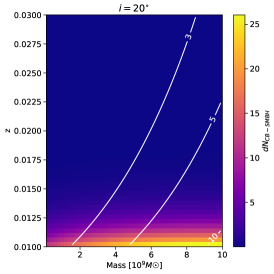
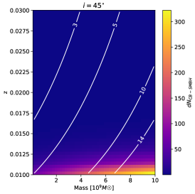
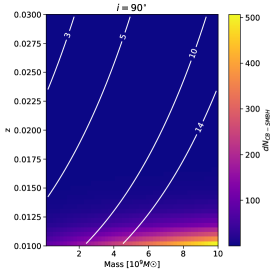
The Figure 1 visualizes (see Section A) the estimated detectability CB-SMBHs with year, a range that is recognized as a ’binary candidate desert’ (see Charisi et al., 2016, and their Figure 12). We find that detectability of such systems is maximized for systems with greater total mass, lower redshifts, and orbits with higher inclinations, as these conditions yield stronger astrometric signals. Overlaid contour lines correspond to constant astrometric wobbles, establishing benchmarks relative to the detection capabilities of the astrometric instruments. The ngEHT is sensitive to wobbles , while GRAVITY+ threshold lies , which is also within the expected performance envelope of GAIA. It is important to note that astrometric wobbles ) are at the threshold of ngEHT detectability, indicating that objects producing such signals are on the cusp of observability. Given that the expected CB-SMBH orbital periods at this GW emission stage are months to years, these objects are accessible via multi-epoch observations with the ngEHT (D’Orazio & Loeb, 2018). As for the GRAVITY+ candidates, CB-SMBH candidates with single, offset, moving broad emission lines (Dexter et al., 2020) are mostly observed at , with apparent magnitudes of and (Runnoe et al., 2017; Guo et al., 2019). In our simulations, we sampled a binary configuration from this specific parameter space with orbital period of year, showcasing the capabilities of future synergies between astrometry and time-domain surveys, for identifying CB-SMBHs in regions once overlooked, thereby contributing to a more comprehensive understanding of binary supermassive black hole populations. However, we also examine one configuration with period 1.3 year, to illustrate the dynamics of systems with periods marginally exceeding our primary interval, shedding light on their characteristics as they converge towards 1 year from above.
2.2 Bayesian Protocol for Simulating and Synthetizing CB-SMBH Multi-instrument Data
We outline a two-tier Bayesian protocol (see also Kovačević et al., 2022a). The first tier involves a Simulator that generates observational multi-instrument data encompassing the astrometric wobble and optical light curves, predicated upon specified characteristics of the CB-SMBH. The second tier, the Bayesian Solver, processes this simulated data to extract ’solutions’ that reveal the decomposed flux of, for instance, the secondary component, along with the orbital parameters of the CB-SMBH.
2.2.1 First tier: Simulator
The CB-SMBH observed astrometric photocenter and flux data are simulated with procedures given in Appendix B. The observed total light curve of CB-SMBH includes the Doppler boosting (Section B.2.1) and stochastic variability (Section B.2.2). We are considering higher line of sight angles, so that detected radiation of CB-SMBH is anticipated to be strongly modulated by Doppler boosting. We note that for face on objects, gravitational redshift and traverse Doppler effects could be more important (Gutiérrez et al., 2022). For stochastic variability, we adopted model describing the stochastic emission of each minidisk in the context of the lamp-post model, thin-disk geometry, and damped random walk (DRW) for the driving function, where the transfer function is assymetric (Chan et al., 2020; Kovačević et al., 2022b). Anticipations of such light curves are substantiated by forthcoming extensive time domain surveys like the LSST (Chan et al., 2020; Kovačević et al., 2022b). The errors for each observed point in the astrometry and time domain data are independent and identically distributed such as that their probability density functions (PDF’s) are normal with mean zero and standard deviations between 3% and 10% of the data (e.g., Dexter et al., 2020; Ivezić et al., 2019). To avoid using exactly the same model to generate the observed data and to find the inverse solution an additional jitter was included in the model when generating the data (see Tuomi et al., 2009).
Regarding the astrometric tracking, the capabilities are advancing to a point where precision can reach as for ng EHT (see D’Orazio & Loeb, 2018, and references therein). With this enhanced capability in mind, we consider binaries of with a physical size of pc at a distance of Mpc. For each black hole in the system, the radii of the inner (, ) and outer edges (, ) of the accretion disks are computed under the assumption of non-spinning black holes ( Section B.2.2): .
The sum of outer radii ld is notably less—by over three orders of magnitude—than the pericenter distance of ld. This ensures that even during the closest approach, the accretion disks are not subject to disruptive tidal forces (see e.g., Wang et al., 2018, 2022), thus substantiating stability of the accretion disks within the binary system.
We strategically selected binary configurations to encompass a range of dynamical behaviors and observational cycles (), which represent the observational time baseline relative to the orbital period of the binary system. Alongside , constant astrometric cadence density of 10 observations per year, is informed by the practical constraints and opportunities presented by current and forthcoming observational facilities (see Fang & Yang, 2022). Despite the potential for acquiring a photometric light curves with very dense LSST cadences, we opt for the adversial photometric cadence identical to astrometry to illustrate our method’s efficacy in data-sparse scenarios. Configurations account that accretion rate ratio of binary components satisfy (Duffell et al., 2020). Configuration focuses on the dynamics of ”q-accrete” as an alternative where the accretion rate of each component is scaled proportionally to its mass, i.e., the fluxes of the binary quasar system are expected to be directly proportional to the masses of the individual black holes (Kelley et al., 2019). In this case, we adopt (Farris et al., 2014b), since the orbital frequency of the binary is still significant (see Figure 9 in Farris et al., 2014b) and the luminosity of the primary mini-disc may also become significant (see Figure 8 in Charisi et al., 2021).
| Configuration | q | [∘] | [∘] | [∘] | [] | [years] | ||
| C1 | 0.3 | 0.25 | 60 | 45 | 60 | 2.28 | 2 | |
| C2 | 0.5 | 0.4 | 30 | 45 | 60 | 1 | 1 | |
| C3 | 0.1 | 0.25 | 30 | 205 | 100 | 9 | 2/3 | |
| C4 | 0.7 | 0.3 | 60 | 105 | 200 | 3.01 | 1/2 | |
| C5 | 0.7 | 0.3 | 60 | 105 | 200 | 2.5 | 1/2 | |
| C6 | 0.7 | 0.67 | 60 | 105 | 200 | 1.3 | 1.5 | |
| General parameters | ||||||||
| flux and astrometry error model | NormalUniform | |||||||
| Wavelength of observed light curve [Å] | ||||||||
| Radiative efficiency of quasar | ||||||||
| Distance to quasar [Mpc] | Mpc | |||||||
| DRW characteristic amplitude | Eq. 22 in Kelly et al. (2009) | |||||||
| DRW time scale[day] | Eq. 25 in Kelly et al. (2009) | |||||||
| DRW mean flux density of quasar light curve [] | ||||||||
| a The LSST u-band filter. | ||||||||
| b is derived from the calculated luminosity of the quasar, which is based on its black hole mass. This luminosity is then converted into a flux density observed at Earth, taking into account the distance of the quasar and the wavelength of the LSST u-band filter. | ||||||||
2.2.2 Second tier: Solver
As already mentioned we use the Solver set of equations for fitting procedure, but without jitter term. Denoting the astrometric observations of photocenter motion by , the flux observations by , then the posterior distribution of the orbital parameters of binary motion and flux of one of components factored out of total flux of binary () via Gaussian process is:
| (7) |
The probability density functions contributing to the equation above could be obtained as follows. The function is the log-likelihood of fitting the astrometry data:
| (8) |
where is the number of observed astrometric data points, and are the observed positions of the photocenter, and are the model-predicted positions of the photocenter using model parameters , and uncertainties of observations are and . Next, a detailed derivation of is provided in Section C (see Eq. C28). This probability density represents the log-likelihood of decomposing from the total flux of a binary system using a Gaussian process with parameters . The prior probability density is a simple product of priors on orbital and GP parameters (see Table 2). Then the posterior distribution , as given by Eq 8, is explored through Bayesian framework in Python PyMC package (Salvatier et al., 2016; Wiecki et al., 2022). This program samples the posterior probability of the model given the data, including prior probabilities for the parameters.
The priors for the orbital parameters are sampled from distributions as given in the Table 2, with parameters based on inspection of both the total light curve and astrometric observation. For example, in the case of C1, the total light curve suggests a relatively stable and symmetric flux behavior, indicating a lower range for eccentricity () and a moderate range for orbital period (). Astrometric observations reveal consistent positional changes indicative of a well-defined orbital plane, constraining parameters such as inclination (). The priors for configuration C1 include a uniform distribution and a normal distribution for centered around 2 years. In addition, priors for and may be constrained to narrower ranges to reflect the stable orbital plane inferred from astrometric data. For the configuration C3, the total light curve exhibits significant flux variations and irregularities, suggesting a wider range for eccentricity () and a longer orbital period () to accommodate the observed dynamical behavior. Astrometric measurements reveal complex positional changes, so that a broader range for and priors is used. The priors for span while could follow a normal distribution centered around 7 years. Additionally, priors for and are to capture the complexity observed in the astrometric data. The error priors are drawn from normal distributions that are centered at expected errors of artificial data and have a standard deviation of .
For the GP model, we did not employ DRW for recovering light curves. The Bayesian framework allows the use of any type of GP kernels. While there is a plethora of GP kernels that can be applied, in this study, we specifically used the squared exponential kernel (SE), which has been tested by Kovačević et al. (2017):
| (9) |
where sets the amplitude of the Gaussian process and has the same units as the flux, and sets the length scale of the Gaussian process and has units of time . The Bayesian framework provides a natural mechanism to determine the most probable values of and through sampling priors of their ranges and optimization of Gaussian process models. For unfavorable configurations, more structured GP kernels could be used such as:
where covariance matrix of Doppler boost for binary parameters is given by .
| Description | Variable | Distribution |
|---|---|---|
| orbital parameters | ||
| mass ratio of components | Uniform | |
| total mass | Normal | |
| eccentricity | Uniform | |
| orbital period | Normal | |
| argument of pericenter | Uniform | |
| longitude of the ascending node | Uniform | |
| GP kernels parametersa | ||
| amplitude of GP kernel for | Normal | |
| amplitude of GP kernel for | Normal | |
| a kernels lenghtscales . | ||
| is average of observed total flux of CB-SMBH. | ||
3 Results
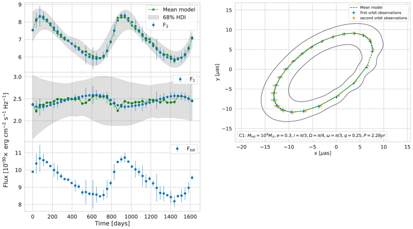
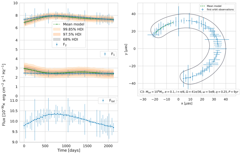
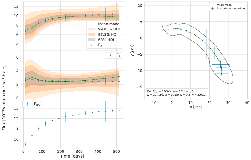
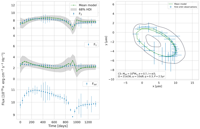
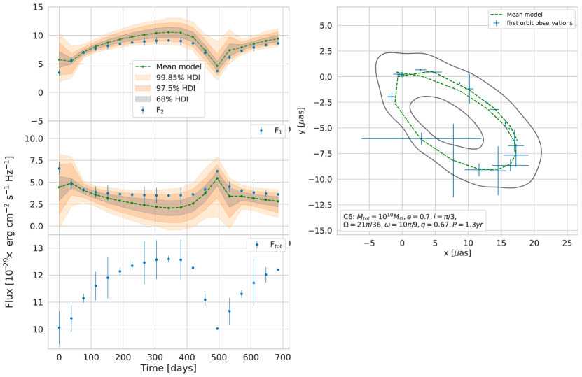
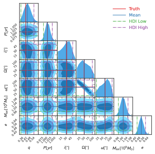
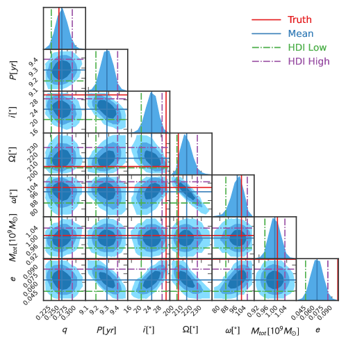
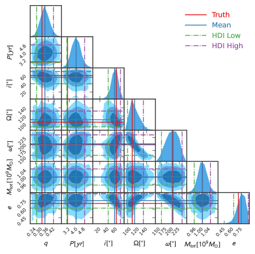
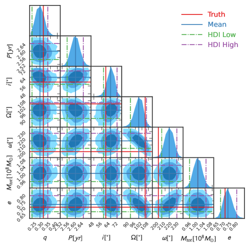
To illustrate the procedure (Section 2.2.2) to recover the orbital parameters and dissolve components fluxes, we consider the six binary configurations listed in Table 1 with varying observational cycles. Disentangled fluxes of the binary components () from the observed total flux are depicted in Figures 2-4. The Bayesian Simulator and Solver employed the PyMC package, which performs Hamiltonian Monte Carlo (HMC) sampling. For sampling, in both tiers of Bayesian code we applied the pymc_ext.optimize non-linear optimization framework for parameter inference (see details in Foreman-Mackey et al., 2021a), which is specifically written for astrophysical applications. It allows us to group astrometric, and emission parameter together, thereby speeding up sampling. We used 4 chains, tuning each for 1000 steps before sampling for a further 40000 steps. The sample have effective sample sizes in the tens of thousands. We report 68% Highest Density Interval (HDI) for posterior values of inferred parameters. In cases such as C3, C4, and C6, we include wider and HDI to avoid underestimating the uncertainty. These intervals align with traditional measures of 1,2 and , respectively. A simplified notation 1, 2, and 3 HDI denotes the 68%, 95 % , and HDI, respectively222The translation from 1 to 3 HDI coverage to conventional sigma () levels is based on the equivalence of probability mass within the HDI in Bayesian statistics to the cumulative probabilities associated with sigma levels in a Gaussian distribution. Specifically, a 68% HDI is analogous to 1, representing approximately 68.27% coverage, a 95% HDI corresponds to 2 ( coverage), and a 99.7% HDI to 3 ( 99.73% coverage). We calculated the effective using the full width of HDI.. The convergence of the Bayesian sampler across scenarios C1-C6 was assessed using two key metrics: the Gelman-Rubin statistic (R-hat) and the effective sample size (ESS). In each scenario, R-hat values were consistently below 1.01 for all parameters, indicating strong convergence and suggesting that the chains mixed well, reaching a stationary distribution. Furthermore, the ESS was several thousands for all parameters, demonstrating that the samples were efficient and informative, providing a solid basis for statistical inferences Figures 7-8 display the Bayesian posterior distributions, and Table 3 details the inferred binary orbital parameters, providing quantitative estimates and their uncertainties. Table 4 evaluates the estimation accuracy of these parameters by indicating their deviation from true values within 1 to 3 HDI distances. Configuration (Fig. 2), characterized by , illustrates long-term dynamic trends. Configurations (Fig. 3) and (Fig. 4), also with , resemble but emphasize different aspects: explores the impact of varying orbital parameters, while represents a ”q-accrete” scenario (Kelley et al., 2019). (Fig. 2) and (Fig. 3) are focused on short-term dynamics (). (Fig. 2), targeting intermediate timescales with , offers a balanced perspective between short-term observational baselines and long-term evolution. In scenario C1, our model captures the fluxes of binary components, reflecting long-term dynamic trends within a system characterized by moderate eccentricity and a lower mass ratio over a period of 2.28 years. This scenario includes two full observational cycles relative to the orbital period. Scenario C2, characterized by higher eccentricity and a slightly higher mass ratio over a 1-year period with one observational cycle, demonstrates the method’s precision in detecting rapid orbital dynamics and flux variations of components within a single cycle, highlighting its ability to capture short-term dynamical behaviors. Scenario C3, with low eccentricity over an extended 9-year period and shows the method’s effectiveness in analyzing systems exhibiting slow orbital dynamics with limited observational cycles. In scenario C4, our approach accurately captures complex orbital dynamics in a binary system with high eccentricity and a mid-range mass ratio over a 3.01-year period, observed within moderate cycles of Scenario C5 underlines the method’s precision across different mass scales in a system with high eccentricity and a lower total mass over a 2.5-year period, with showcasing its ability to decompose fluxes accurately even in sparsely observed cycles. Finally, C6 focuses on a massive binary system with a short period of 1.3 years and illustrating the method’s adaptability in monitoring flux variations of components across more frequent observing cycles in scenarios involving very high binary mass and rapid orbital periods.
(a)

(b)
(a)
(b)
(a)
(b)
| Configuration | [yr] | ||||||
|---|---|---|---|---|---|---|---|
| C1 | |||||||
| C2 | |||||||
| C3 | |||||||
| C4 | |||||||
| C5 | |||||||
| C6 |
| Configuration | |||||||
|---|---|---|---|---|---|---|---|
| C1 | 1 HDI | 1 HDI | 1 HDI | 1 HDI | 1 HDI | 1 HDI | 1 HDI |
| C2 | 1 HDI | 1 HDI | 1 HDI | 1 HDI | 1 HDI | 1 HDI | 1 HDI |
| C3 | 1 HDI | 1 HDI | 1 HDI | 1 HDI | 1 HDI | 2 HDI | 1 HDI |
| C4 | 1 HDI | 1 HDI | 1 HDI | 1 HDI | 1 HDI | 2 HDI | 1 HDI |
| C5 | 1 HDI | 1 HDI | 1 HDI | 1 HDI | 1 HDI | 1 HDI | 1 HDI |
| C6 | 3 HDI | 2 HDI | 1 HDI | 1 HDI | 1 HDI | 2 HDI | 2 HDI |
4 Discussion
Here, we discuss observational strategies, the expected astrometric wobble distributions within the parameter space of CB-SMBH and address potential limitations in our methodology.
4.1 Comparison of Observational Strategies
Our Bayesian synthesis method successfully estimated the orbital parameters of the binary quasar system across six configurations (Table 1), demonstrating the model’s capability to accurately recover parameters (Table 3). The estimated values are generally in close agreement with the true values (Figure 7-9, with most parameters falling within the 1HDI and confidence intervals ranging from 1HDI to, in a few cases, 2-3HDI for more challenging configuration of ”q-accrete” C6 (Table 4). Configuration C1 benefits from an optimal match between observing cycles and the orbital period, supported by moderate eccentricity and mass ratio. This balance enables precise components fluxes decomposition within HDI, highlighting the effectiveness of the observational strategy in capturing the binary’s stable dynamics over two complete cycles. C2 demonstrates the model’s ability to accurately capture rapid dynamical changes within a shorter, 1-year period with a single observing cycle. The higher eccentricity here necessitates dense observational coverage, which is achieved, resulting in flux decompositions aligning within HDI. C3 faces challenges due to its extended 9-year period and a lower , which complicates the full capture of long-term dynamics, placing decomposed fluxes within at the beginning of observing cycle. This reflects the difficulty in tracking the binary’s evolution with sparser data points. C4 and C5 contend with high eccentricity (, impacting the flux decomposition’s precision. The longer period and half-cycle observing rates introduce complexities in fully capturing the binary’s dynamics, likely resulting in decomposed fluxes aligning within sigma in the case of C4. However, due to smaller period of C5 the cadence is enough granular to decompose fluxes within HDI.Additionally, the relatively higher eccentricity and lower total mass in C5 compared to other configurations may contribute to more distinguishable flux variations that are easier to capture within the given observational sampling. C6, with a higher and a significant mass of ’q-accrete’ within a compact 1.3-year period, faces intense dynamical variations. The alignment of decomposed fluxes within wider sigma bands for C6 indicates the model’s capacity to account for these rapid variations to a certain extent. However, the deviations from tighter sigma bands underscore the necessity for more nuanced observational strategies, such as increasing the sampling rate during critical phases or employing predictive modeling to enhance the temporal resolution of observations. Given the uncertainty surrounding the specific type of binary system at the outset of observation, the configurations examined here point out the importance of a flexible and adaptive observational approach, capable of accommodating the wide range of binary characteristics that might be encountered:
-
•
Start with a baseline sampling rate, such as the 10 observations per year, and adjust based on early data analysis. If rapid flux variations or complex orbital dynamics are detected, increase the observation frequency accordingly.
-
•
Multi-wavelength observations can provide additional clues about the binary system’s nature, aiding in the refinement of observational strategies to better target the detected features.
-
•
Collaborations that allow for shared data and observations from different facilities and instruments can enhance the detection capabilities and flux decomposition.
An example of workflow could involve collecting LSST catalogue data on variability, and providing this information to future astrometry facilities. These facilities can then use the catalogue to optimize their observing strategy in real time based on modeling, ensuring efficient capture of dynamic binary behavior.
4.2 Distributions of Expected Astrometric Wobble
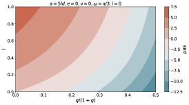
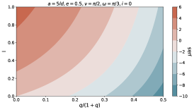
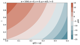
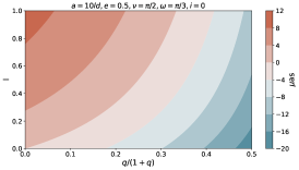
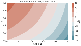
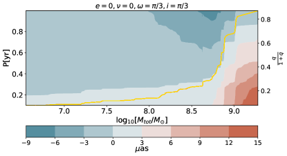
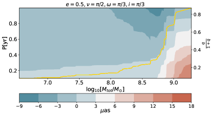
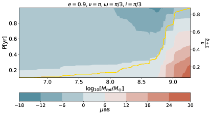
Here we predict and examine the astrometric wobbles of CB-SMBH across two distinct parameter spaces: the plane, and the total mass-period domain. Within each space, we incorporate variations in eccentricity and orbital phase. The purpose of the predictions is to assist and enhance multi-instrument observational strategies.
For the computations of the offset across a grid of binary parameters, a simplified equation Eq. B10 is employed, wherein the luminosity parameter is assumed to be time-invariant, and both the luminosity and mass ratios are presumed to have a uniform distribution. This assumption allows us to focus exclusively on the dynamical parameters of the orbit—namely, the semi-major axis , eccentricity , true anomaly 333Equivalent term is orbital phase., inclination , and orbital orientation . The formula for total photocenter displacement could have positive or negative sign depending on the values of and . If , then the component with the larger mass contributes less to the total light of the system, and vice versa.
Given that the most significant effects are expected from objects within tens of Mpc (Dexter et al., 2020), we set the distance of the object to be roughly 70 Mpc. We then compute the offsets (Eq. B10) for various binary parameters combinations in the plane, under the assumption of a fixed inclination .
In Figure 5, the distinction between offsets for different values of the semi-major axis is clear. In the top row, where ld, the offsets are consistently lower than in the bottom row, with ld, emphasizing the influence of semimajor axis on the offsets.
The variation in eccentricity and true anomaly across the columns of Figure 5 illustrates the influence of these parameters on the resultant offsets. The uniformity in the first column (subplots a, d) for a circular orbit contrasts with the pronounced variation observed in the second (subplots b, e) and third columns (subplots c, f), especially at higher eccentricities. At a moderate eccentricity and a true anomaly , the offset variation is more pronounced, especially when comparing it with the circular case in the first column. The slight differences between subplots (b) and (e) further highlight the enhanced offset sensitivity to the orbital phase at this eccentricity. With a high eccentricity and the orbital phase close to , the offset values display a contrast, in both subplots (c) and (f) with respect to other cases. This underscores the pronounced effects of having components near the apocenter of their elliptical orbit, producing more substantial displacements.
 |
 |
 |
| (a) | (b) | (c) |
 |
 |
 |
| (d) | (e) | (f) |
We now focus on the photocenter displacement,, as a function of the total mass and period, (see Figure 6). This alternative phase plane is crucial due to its direct link to the binary’s physical and orbital parameters. For this analysis, we reparametrize the binary’s relative position, , in Eq. B10 using the formula:
| (10) |
This equation shows the dependencies on the total mass , orbital period , eccentricity , and the true anomaly . In an eccentric orbit, the radius fluctuates, peaking at (the apocenter). Hence, the maximum displacements may occur when the binary system’s orbit is highly eccentric (), and the orbital phase, defined by the true anomaly , is at . This aligns with the apocenter, where the two bodies in the binary system are maximally separated.
Based on Figure 6, we outline several trends dictated by dynamical parameters. In the top subplot, for circular systems encompassing total masses within to , there exists a balanced distribution of positive and negative offsets. However, this gets disrupted for masses in the range from to , wherein a pronounced tendency to positive offsets emerges. This suggests that as we progress to more massive systems, the distinction between the light-weighted center and mass-weighted center becomes more pronounced.
Increasing the eccentricity to 0.5 introduces deviations from circularity in the orbits. This scenario is set at . Here, the positive offset regions have enlarged compared to top subplot, especially for higher mass systems. This trend underscores the perturbative effects of higher eccentricities: as orbits deviate from perfect circles, gravitational interactions over the orbit become more varied, leading to pronounced photocenter displacements. The bottom subplot captures the systems at the most elliptical scenario, with the diametrically opposed components positions. The significant eccentricity profoundly impacts the offset distributions. The positive offset region has not only enlarged but also stretched towards higher masses. Notably, the boundaries defined by the yellow curve, representative of the barycenter parameter are most prominent here, illustrating how the offset distributions are inherently tied to this parameter, especially at such high eccentricities.
The plane of reveals that the demarcation between positive and negative total offset values are delineated with the mass ratio . Specifically, if , then the component with the larger mass contributes less to the total emission of the system, and the total photocenter displacement will be positive. This may suggest that the more massive component is less luminous (or active) or possibly obscured. On the other hand, if , then the component with the larger mass contributes more to the total light of the system, and the photocenter displacement will be negative. This may suggest that the more massive component is more luminous (active) or less obscured. This relationship is particularly pronounced for total masses exceeding and periods year, as larger masses and extended periods lead to larger orbital separations and, consequently, more significant photocenter displacements. Since our method provides the mass ratio and disentangles the light curve of the secondary, total photocenter enables us to derive a preliminary indicator of the activity of the components in the CB-SMBH system.
(a)
(b)
(c)
4.3 Caveats
Here we highlight further aspects that can modulate the interpretation of our results.
-
•
Orbital Phase Dependancy: The photocenter offset exhibits a dependence on the orbital phase, with smaller variations at the pericenter compared to the apocenter. This could be seen from the ratio of photocenter offset values in pericenter and apocenter inferred from Eq.B10:
(11) However, we also see that for CB-SMBH systems with mild eccentric orbits (), the offset ratio tends to approach unity, implying that even at pericenter, the observed offset can be relatively nonneglibile. This phase-dependent behavior necessitates careful consideration when interpreting observed offsets, especially for systems with varying eccentricities (see related discussions in Kovačević et al., 2022a).
-
•
Parallax and Proper Motion: Our analysis did not account for the possibility of parallax and proper motion. While we assumed that most short-period CB-SMBH systems exhibit small and likely imperceptible parallax, still, we cannot exclude the existence of systems with larger parallax. Furthermore, proper motion of quasars may arise from various sources, such as differential variability between close sources (see Makarov & Secrest, 2022), or due to the motion of a relativistic jet, as in the case of PKS 0119+11 Lambert et al. (2021), which could affect proper motion measurements. These factors merit further investigation and consideration when interpreting photocenter offset measurements (see Makarov & Secrest, 2022; Lambert et al., 2021). According to Makarov & Secrest (2022) many proper motion quasars may be unresolved dual systems displaying the variable imposed motion effect, while a smaller number may be coincidence alignments with foreground stars creating weak gravitational lensing.
-
•
Low-Mass Galaxies with Black Holes: Our study primarily focused on massive CB-SMBH systems; however, it is essential to recognize that low-mass galaxies hosting black holes with masses approaching may require a separate examination. Several campaigns in recent years (see e.g., Reines et al., 2013; Molina et al., 2021) have shown that 50–80 percent of low-mass galaxies may harbor in their core low mass black holes with masses approaching (see Xin & Haiman, 2021, and references therein). These black holes follow scaling relations similar to SMBHs (see e.g. Volonteri & Natarajan, 2009) and could impact the study of binary candidates, given their unique characteristics and potential contribution to active galactic nuclei (see Kimbrell et al., 2021).
-
•
Large Binary Separations and Disc Alignment: The dynamics of CB-SMBH systems may change significantly at large binary separations or periods. Circumbinary gas accretion can dominate over gravitational wave emission, and the alignment of circumbinary discs with the orbital plane introduces complexities that deserve further investigation. Such systems may require a distinct treatment within the CB-SMBH framework (see Aly et al., 2015; D’Orazio & Di Stefano, 2017; Miller & Krolik, 2013). For example, any periodic emission from the binary mini-discs or the circumbinary disc’s inner edge will be obscured if the binary orbit is co-planar with a circumbinary disc.
-
•
Variability of Accretion Discs: In cases where the source periodicity is primarily driven by the variability of the accretion disc rather than the Doppler boost, modeling the motion of the photocenter becomes challenging. The resulting curve may exhibit substantial noise and not form a closed ellipse, affecting our ability to model and interpret photocenter motion accurately (see also discussion in Kovačević et al., 2022a).
-
•
Detection of Ultra-Compact Binaries: Extremely ultra-compact binary systems with very short periods (see details in Xin & Haiman, 2021) may present challenges for astrometric detection. The expected offsets for such systems may fall below the detection threshold for current astrometric instruments (e.g., GAIA threshold is as, see D’Orazio & Loeb, 2019). Therefore, time-domain optical surveys like LSST and future gravitational wave observatories like LISA (Amaro-Seoane et al., 2017) may be necessary for detection and study of such systems.
-
•
Newtonian and Relativistic Precession: Our analysis did not consider the effects of Newtonian precession or relativistic precession in compact binary systems. These effects can introduce additional complexities into the observed variability, and further investigation is required to assess their significance (see the example of OJ287 Laine et al., 2020).
-
•
Contribution of Circumbinary Structures: The potential contribution of circumbinary structures, such as circumbinary disks or circumbinary broad line regions, to the emission from CB-SMBH systems could impact the observed photocenter motion. The extent of this impact and its implications for binary framework studies remain subjects for future exploration (Dexter et al., 2020; Kovačević et al., 2022a; Popović et al., 2021; Simić et al., 2022; Guo et al., 2022).
5 Conclusions
We developed a two-tier Bayesian framework for the synthesis of multi-instrument observational data from CB-SMBH systems. The Simulator, as the first tier, is generating synthetic datasets that replicate the astrometric wobble and total optical light curves of these systems. The second tier, the Solver, uses these datasets to infer individual fluxes of binary components and binary orbital parameters with reliable precision, as evidenced by our simulation’s posterior distributions.
In summary, these are our conclusions:
-
•
Our Bayesian synthesis method reliably determines binary orbital parameters and extract individual fluxes of binary components from the total flux, within multi, intermediate and short-term observational cycles with respect to orbital period, assuming density of observations 10 per year in astrometry and photometry. For configurations with longer periods, lower eccentricity and mass ratios, the method accurately tracks component fluxes within 1 HDI. In configurations with higher eccentricity and mass ratio over a one-year period, it demonstrates rapid dynamic analysis capabilities, also achieving decompositions of fluxes within 1 HDI. Configurations with higher eccentricities and intermediate obsevrational baselines () result in decompositions of components fluxes within 2 HDI. Case with short period, high eccentricity, and significant mass, particularly in ”q-accrete” scenario with , show the method’s robustness in capturing swift variations, with decompositions of fluxes of components aligning within 3 HDI.
-
•
The configurations analyzed highlight the need for adaptable observational strategies to accommodate diverse binary system characteristics. Key considerations include beginning with a standard observation rate (e.g. 10 observations per year) but remaining flexible to adjust based on initial data analysis. Increased frequency may be used for systems showing rapid flux variations or complex orbital dynamics. Using multi-wavelength observations can provide insights into the binary system’s nature, informing adjustments to observational strategies for better targeting observed features. An illustrative workflow might involve leveraging LSST catalogue data on variability to inform real-time optimization of observing strategies by future astrometry facilities.
-
•
The astrometric wobble is particularly sensitive to factors such as the semi-major axis, eccentricity, and orbital phase, with the largest values occurring in highly eccentric orbits at the apocenter. Association between the binary mass ratio and total photocenter offset, suggests that the more massive component’s contribution to the system’s total light curve is inversely related to its luminosity. This trend is especially pronounced in systems with total masses and periods of 1 year, where larger masses and longer periods typically result in greater photocenter displacements. We show that this can provide preliminary information on components’ activity.
Our Bayesian approach shows the potency of multi-instrument data integration and allows for CB-SMBH observational timelines over 1-2 orbital periods, even for systems with periods year. Such a synthesis can assist in extracting information from upcoming large-scale time-domain surveys, like LSST, and next-generation interferometers, such as ng-EHT and GRAVITY+.
Appendix A Number of CB-SMBH with astrometric wobble
At angular-diameter distance , and the binary orbital projected angular extent is . The astrometric wobble above the given threshold is . Then, instrument can detect astrometric wobble if and if the orbital period the half of instrument observational timeline. We use the quasar luminosity function (Hopkins et al., 2007; Xin & Haiman, 2021)to derive the number of AGN per redshift and luminosity .At each total binary mass bin we derive luminosity from the assumption that the AGN emits at a fraction of Eddington luminosity, , where for the Eddington fraction of bright AGN we adopt . We assume that quasars typically have a total lifetime of years (independent of redshift and luminosity), and that their residence time at given is
| (A1) |
Under these assumptions, the number of quasars with orbital periods year, and is given approximately by
| (A2) |
The differential comoving volume element is calculated for cosmological parameters , , (Planck Collaboration et al., 2020) via astropy.cosmology module.
With this approximation, we compute the distribution of the number of CB-SMBH in a grid of mass bins evenly distributed across in log-space, and redshift bins in , respectively.
Appendix B Simulator of CB-SMBH astrometric data and light curve
B.1 Simulation of CB-SMBH Astrometric Data
The CB-SMBH is assumed to be a two-body system of SMBHs, such that their masses satisfy . The procedure for simulating astrometric data is discussed briefly below, and further information may be found in Kovačević et al. (2020b).
| Parameter | Units | Name | fiducial range |
|---|---|---|---|
| ld pc | semimajor axis | ||
| - | eccentricity | ||
| yr days | orbital period | ||
| ∘ | argument of pericenter | ||
| ∘ | inclination | ||
| ∘ | angle of ascending node | ||
| days yr | time of pericenter passage |
Naturally, dynamical parameters fully describe the SMBH position relative to the barycentre of system (see Table 5). The apparent relative orbit is the one of the secondary around the primary projected on the sky plane, and it can be determined from measurements of the relative position of the components obtained through astrometric imaging or interferometric observations. The projected spatial motion of the binary components is calculated within the reference frame centered on the primary component or barycentre and two axes in the plane tangent to the celestial sphere (Le Bouquin et al., 2013): the -axis points north, while the -axis points east. The -axis runs parallel to the line of sight and points in the direction of rising radial velocities (positive radial velocities). Here we provide equation in the barycenter reference frame.
The transformations could be represented in the vectors and (Thiele-Innes parameters) instead of utilizing cosine and sine terms of Euler rotations.
The vector of relative position of an SMBH w.r.t barycentre is:
| (B1) |
where is the eccentric anomaly determined from the Kepler equation , and is set to for simplicity. The vectors of barycenter position and velocity are set to zero for simplicity. Thiele-Innes functions and are defined as follows:
| (B2) | |||||
| (B3) | |||||
| (B4) | |||||
| (B5) |
where we assume that is semimajor axis of secondary component, and . Therefore, above equations describe relative orbit of secondary with respect to primary. The data matching the third coordinate of body position ( ) can not be obtained.
The model for photocenter motion is now simply
where is a distance, , , and .
We assume that both masses, and distance are known and that fluxes of both SMBH are obtained via simulation procedure given in Appendix B.2.2. We assume that the errors for each artificial observation are independent and identically distributed, resembling white noise at the level of (see also Dexter et al., 2020). In order to avoid using the same model for both producing the observations and finding the solution, an additional jitter was added in the model when simulating the data.
B.1.1 Approximation of Photocenter Motion Using True Anomaly
In this section, we will re-approximate the motion of the photocenter using the true anomaly (). It represents the angle between the direction of periapsis (the point of closest approach to the central body) and the current position of the object. As such, it is a more intuitive parameter that can be visualized and understood easily. More importantly, the true anomaly proves particularly useful for predicting an object’s future position on its orbit. This property is advantageous for the general exploration of the parameter grid space of CB-SMBH. The use of true anomaly allows for a more straightforward and less computationally-intensive approximation.
Let the two components of binary are at the relative position given by , where T mark transposition, is orbit orientation matrix of binary, and is a polar coordinates in the orbital plane as given in Appendix A in Kovačević et al. (2020b). We then rewrite the components given in Eq. B1 in terms of orbital phase :
| (B6) | |||
| (B7) | |||
| (B8) |
Then we will calculate the total photocenter motion as :
| (B9) | ||||
| (B10) |
B.2 Simulation of CB-SMBH light curve
At higher viewing angles, the detected binary radiation would be strongly modulated by relativistic effects such as gravitational lensing and Doppler boosting. Here, we consider the case when the emission coming from two minidiscs surrounding each component in the system will appear Doppler boosted (Haiman et al., 2009; Hu et al., 2020). We schematically decompose the total observed flux of binary as (see, e.g. Hu et al., 2020; Gutiérrez et al., 2022)
| (B11) | ||||
| (B12) |
where the , account for stochastic variability, corresponding average values and Doppler boost term of each minidisc in the system, respectively.
The next two sections provide formulas for Doppler brightnening and stochastic variability calculation for each minidisk.
B.2.1 Doppler boost
At a given photon frequency , assuming that the minidisc emission is the Doppler effect is (D’Orazio & Di Stefano, 2018)
| (B13) |
where , , and are the power law spectrum index, orbital inclination, phase of binary, and 3D velocity of component, respectively. The projection of the velocity vector onto the line of sight is given as
| (B14) | ||||
| (B15) | ||||
| (B16) |
is the argument of pericenter, and is the true anomaly. We solve for the radial velocity for both binary components, prescription given in Kovačević et al. (2022a, 2020a) for binary mass ratio . Both components are assumed to be Doppler-modulated with corresponding line-of-sight velocities and that emission from both black holes share the same spectral index with a value of the composite quasar spectrum (Vanden Berk et al., 2001).
B.2.2 Stochastic variability
It is predicted that the quasars high-quality light curves obtained from the LSST and other large time domain facilities will be not only shifted in time but also distorted at different wavelengths (Chan et al., 2020; Kovačević et al., 2022b). We adopted this approach to model the stochastic emission of each minidisk in the context of the lamp-post model, thin-disk geometry,and damped random walk (DRW) for the driving function, where the size of the transfer function expands with wavelength.
For this purposes we will introduce auxiliary scaling factors. To approximate the mass accretion rate of the binary system in terms of the total mass of the binary , we can use the Eddington accretion rate:
| (B17) |
where is the proton mass, is the Thompson scattering cross-section, and is a typical radiative efficiency of quasar, and is a constant. For the symmetrical binary systems , it is expected that , and as the decreases, the ratio increases (Raimundo & Fabian, 2009; Shankar et al., 2009; Duffell et al., 2020). Therefore, if the implied accretion rate of the binary is , then the accretion rate is split between the two black holes with where and . We assume that as given in Duffell et al. (2020), if not otherwise stated. Each minidisk in a binary is set up as a non-relativistic thin-disk emitting black-body radiation (Shakura & Sunyaev, 1973; Thorne, 1974), with the central source treated as a ”lamp post” placed near the black hole (Cackett et al., 2007; Starkey et al., 2017). Then, the temperature profiles of each minidisk are described as (Chan et al., 2020; Kovačević et al., 2022b; Starkey et al., 2017; Cackett et al., 2007; Davelaar & Haiman, 2022)
| (B18) |
where the scale radius is
| (B19) |
is the rest frame wavelength, is the Stefan-Boltzmann constant, is Boltzmann constant, is a gravitational constant, is total mass of the binary, is the inner radius of minidisk surrounding mass and
| (B20) |
Using Eqs. B18-B20 and following prescription in Chan et al. (2020); Kovačević et al. (2022b), the transfer function for each disc at given is:
| (B21) | ||||
| (B22) | ||||
where the outer disc radius is approximated as (Jiménez-Vicente et al., 2014), is azimuth of reprocessing site, is inclination of the disc.
Finally, assuming that each minidisk has an own driving-source emission , the total minidisc flux is obtained by convolution Tie & Kochanek (2018):
| (B23) |
Here, is the fractional luminosity variability ‘lagged’ by the light travel time from the disc center. We represent this driving light curve by the Damped Random Walk (DRW) model with the characteristic amplitude and timescale (Kelly et al., 2009; Kozłowski, 2017). The DRW is constructed from the procedure given in Kovačević et al. (2021).
Appendix C Additive decomposition of CB-SMBH light curves using GP
Here we provide an auxiliary formula for Gaussian conditional (Section C.1), which enables us to model the conditional distribution of one GP component given the sum of GPs. Then we proceed with the likelihood of additive decomposition of CB-SMBH light curves via GPs (Section C.2), which provides a means to estimate the individual components from the sum of the light curves of both SMBH in binary system.
C.1 Gaussian Conditional
Here we provide an auxiliary formula for the multivariate Gaussian conditional distribution , which is used for likelihood of additive decomposition of Gaussian process (see Rasmussen, 2004; Mardia et al., 1979; Duvenaud et al., 2013).
Let follow a multivariate normal distribution:
| (C1) |
Then, the conditional distribution of any subset vector , given the complement vector , is also a multivariate normal distribution:
| (C2) |
where the conditional mean and covariance are:
| (C3) | ||||
with block-wise mean and covariance defined as:
| (C4) | ||||
To prove the concept of C3, we will assume that C4 and following equation holds:
| (C5) |
where is an vector, is an vector, and is an vector. Then, we recall that by construction, the joint distribution of and is:
| (C6) |
Moreover, the marginal distribution of follows from a multivariate normal distribution C1 and C4 as
| (C7) |
According to the Bayes law of conditional probability, it holds that
| (C8) |
Using the probability density function of the multivariate normal distribution, we get:
| (C10) |
Writing the inverse of as
| (C11) |
| (C12) |
Rearranging C12, we have
| (C13) |
We also recalll that the determinant of a block matrix is:
| (C15) |
| (C16) |
where
With , because is a covariance matrix, and , we finally arrive at
| (C17) |
The above equation is the probability density function of a conditional multivariate normal distribution:
| (C18) |
with the mean and covariance given by (C3).
C.2 Likelihood of Decomposition of CB-SMBH Light Curve via GP
Let the CB-SMBH observed light curve is , and a priori unknown and independent emissions from components are given as at observed time instances . We assume that the light curves have the following Gaussian Process representation (Rasmussen, 2004):
| (C19) | ||||
| (C20) | ||||
| (C21) |
where is Gaussian distribution with mean function and covariance functions (also called the kernels). Any number of components in multiple systems can be summed this way. In what follows, we distinguish between flux values at training locations and the flux values at some set of query locations
Then, the joint prior distribution over two unknown component light curve drawn independently from GP priors, and their sum is given by (Duvenaud et al., 2013):
| (C23) | ||||
where
| (C24) | |||
| (C25) | |||
| (C26) |
Now, using formula for Gaussian conditional (see Eq. C17-C18), the conditional distribution of unknown light curves () conditioned on their sum is given as:
| (C27) | ||||
From above equation, the log-likelihood of the conditional distribution of given at the query time instances is easily obtained:
| (C28) | ||||
where the number of observed points is , the variance and mean of given are
and
, respectively. This loglikelihood of the component of the signal is integrating (marginalizing) over the possible configurations of the other components.
Appendix D Posterior sampling statistics
Here, we present the posterior distributions of binary parameters inferred through the Bayesian Solver procedure (see Section 2.2.2) for configurations C1-C6 (Table 1), encompassing a variety of optical time domain and astrometry data observational baselines (see Figs. 2-4).

(a)
(b)
(a)
(b)
(a)

(b)
References
- Aly et al. (2015) Aly, H., Dehnen, W., Nixon, C., & King, A. 2015, MNRAS, 449, 65, doi: 10.1093/mnras/stv128
- Amaro-Seoane et al. (2017) Amaro-Seoane, P., Audley, H., Babak, S., et al. 2017, arXiv e-prints, arXiv:1702.00786. https://arxiv.org/abs/1702.00786
- Arzoumanian et al. (2020) Arzoumanian, Z., Baker, P. T., Blumer, H., et al. 2020, ApJ, 905, L34, doi: 10.3847/2041-8213/abd401
- Begelman et al. (1980) Begelman, M. C., Blandford, R. D., & Rees, M. J. 1980, Nature, 287, 307, doi: 10.1038/287307a0
- Belokurov et al. (2020) Belokurov, V., Penoyre, Z., Oh, S., et al. 2020, Monthly Notices of the Royal Astronomical Society, 496, 1922, doi: 10.1093/mnras/staa1522
- Bianco et al. (2022) Bianco, F. B., Ivezić, Ž., Jones, R. L., et al. 2022, ApJS, 258, 1, doi: 10.3847/1538-4365/ac3e72
- Bogdanović et al. (2011) Bogdanović, T., Bode, T., Haas, R., Laguna, P., & Shoemaker, D. 2011, Classical and Quantum Gravity, 28, 094020, doi: 10.1088/0264-9381/28/9/094020
- Bogdanović et al. (2022) Bogdanović, T., Miller, M. C., & Blecha, L. 2022, Living Reviews in Relativity, 25, 3, doi: 10.1007/s41114-022-00037-8
- Bowen et al. (2017) Bowen, D. B., Campanelli, M., Krolik, J. H., Mewes, V., & Noble, S. C. 2017, ApJ, 838, 42, doi: 10.3847/1538-4357/aa63f3
- Bowen et al. (2018) Bowen, D. B., Mewes, V., Campanelli, M., et al. 2018, ApJ, 853, L17, doi: 10.3847/2041-8213/aaa756
- Bowen et al. (2019) Bowen, D. B., Mewes, V., Noble, S. C., et al. 2019, ApJ, 879, 76, doi: 10.3847/1538-4357/ab2453
- Broderick et al. (2020) Broderick, A. E., Pesce, D. W., Tiede, P., Pu, H.-Y., & Gold, R. 2020, The Astrophysical Journal, 898, 9, doi: 10.3847/1538-4357/ab9c1f
- Burke-Spolaor et al. (2019) Burke-Spolaor, S., Taylor, S. R., Charisi, M., et al. 2019, A&A Rev., 27, 5, doi: 10.1007/s00159-019-0115-7
- Cackett et al. (2007) Cackett, E. M., Horne, K., & Winkler, H. 2007, MNRAS, 380, 669, doi: 10.1111/j.1365-2966.2007.12098.x
- Chan et al. (2020) Chan, J. H. H., Millon, M., Bonvin, V., & Courbin, F. 2020, A&A, 636, A52, doi: 10.1051/0004-6361/201935423
- Charisi et al. (2016) Charisi, M., Bartos, I., Haiman, Z., et al. 2016, Monthly Notices of the Royal Astronomical Society, 463, 2145, doi: 10.1093/mnras/stw1838
- Charisi et al. (2021) Charisi, M., Taylor, S. R., Runnoe, J., Bogdanovic, T., & Trump, J. R. 2021, Monthly Notices of the Royal Astronomical Society, 510, 5929, doi: 10.1093/mnras/stab3713
- Chen et al. (2020) Chen, Y.-C., Liu, X., Liao, W.-T., et al. 2020, MNRAS, 499, 2245, doi: 10.1093/mnras/staa2957
- Davelaar & Haiman (2022) Davelaar, J., & Haiman, Z. 2022, Phys. Rev. Lett., 128, 191101, doi: 10.1103/PhysRevLett.128.191101
- De Rosa et al. (2019) De Rosa, A., Vignali, C., Bogdanović, T., et al. 2019, New Astronomy Reviews, 86, 101525, doi: https://doi.org/10.1016/j.newar.2020.101525
- Dexter et al. (2020) Dexter, J., Lutz, D., Shimizu, T. T., et al. 2020, ApJ, 905, 33, doi: 10.3847/1538-4357/abc24f
- D’Orazio & Di Stefano (2017) D’Orazio, D. J., & Di Stefano, R. 2017, MNRAS, 474, 2975, doi: 10.1093/mnras/stx2936
- D’Orazio & Di Stefano (2018) D’Orazio, D. J., & Di Stefano, R. 2018, MNRAS, 474, 2975, doi: 10.1093/mnras/stx2936
- D’Orazio et al. (2013) D’Orazio, D. J., Haiman, Z., & MacFadyen, A. 2013, MNRAS, 436, 2997, doi: 10.1093/mnras/stt1787
- D’Orazio et al. (2015) D’Orazio, D. J., Haiman, Z., & Schiminovich, D. 2015, Nature, 525, 351, doi: 10.1038/nature15262
- D’Orazio & Loeb (2019) D’Orazio, D. J., & Loeb, A. 2019, Phys. Rev. D, 100, 103016, doi: 10.1103/PhysRevD.100.103016
- Duffell et al. (2020) Duffell, P. C., D’Orazio, D., Derdzinski, A., et al. 2020, ApJ, 901, 25, doi: 10.3847/1538-4357/abab95
- Dullo et al. (2017) Dullo, B. T., Graham, A. W., & Knapen, J. H. 2017, MNRAS, 471, 2321, doi: 10.1093/mnras/stx1635
- Duvenaud et al. (2013) Duvenaud, D., Lloyd, J., Grosse, R., Tenenbaum, J., & Zoubin, G. 2013, in Proceedings of Machine Learning Research, Vol. 28, Proceedings of the 30th International Conference on Machine Learning, ed. S. Dasgupta & D. McAllester (Atlanta, Georgia, USA: PMLR), 1166–1174. https://proceedings.mlr.press/v28/duvenaud13.html
- D’Orazio & Loeb (2018) D’Orazio, D. J., & Loeb, A. 2018, The Astrophysical Journal, 863, 185, doi: 10.3847/1538-4357/aad413
- EHT Collaboration et al. (2019) EHT Collaboration, Akiyama, K., Alberdi, A., et al. 2019, The Astrophysical Journal Letters, 875, L1, doi: 10.3847/2041-8213/ab0ec7
- Eilers et al. (2023) Eilers, A.-C., Simcoe, R. A., Yue, M., et al. 2023, ApJ, 950, 68, doi: 10.3847/1538-4357/acd776
- Fang & Yang (2022) Fang, Y., & Yang, H. 2022, The Astrophysical Journal, 927, 93, doi: 10.3847/1538-4357/ac4bd7
- Farris et al. (2014a) Farris, B. D., Duffell, P., MacFadyen, A. I., & Haiman, Z. 2014a, MNRAS: Letters, 447, L80, doi: 10.1093/mnrasl/slu184
- Farris et al. (2014b) —. 2014b, The Astrophysical Journal, 783, 134, doi: 10.1088/0004-637X/783/2/134
- Ferré-Mateu et al. (2015) Ferré-Mateu, A., Mezcua, M., Trujillo, I., Balcells, M., & van den Bosch, R. C. E. 2015, ApJ, 808, 79, doi: 10.1088/0004-637X/808/1/79
- Foreman-Mackey et al. (2021a) Foreman-Mackey, D., Luger, R., Agol, E., et al. 2021a, arXiv e-prints, arXiv:2105.01994. https://arxiv.org/abs/2105.01994
- Foreman-Mackey et al. (2021b) —. 2021b, arXiv e-prints, arXiv:2105.01994. https://arxiv.org/abs/2105.01994
- Gaia Collaboration et al. (2016) Gaia Collaboration, Prusti, T., de Bruijne, J. H. J., et al. 2016, A&A, 595, A1, doi: 10.1051/0004-6361/201629272
- Gaia Collaboration et al. (2021) Gaia Collaboration, Brown, A. G. A., Vallenari, A., et al. 2021, A&A, 649, A1, doi: 10.1051/0004-6361/202039657
- Ge et al. (2019) Ge, X., Zhao, B.-X., Bian, W.-H., & Frederick, G. R. 2019, AJ, 157, 148, doi: 10.3847/1538-3881/ab0956
- Gezari et al. (2007) Gezari, S., Halpern, J. P., & Eracleous, M. 2007, ApJS, 169, 167, doi: 10.1086/511032
- Ghisellini et al. (2009) Ghisellini, G., Foschini, L., Volonteri, M., et al. 2009, MNRAS, 399, L24, doi: 10.1111/j.1745-3933.2009.00716.x
- Ghisellini et al. (2015) Ghisellini, G., Tagliaferri, G., Sbarrato, T., & Gehrels, N. 2015, MNRAS, 450, L34, doi: 10.1093/mnrasl/slv042
- Graham et al. (2015) Graham, M. J., Djorgovski, S. G., Stern, D., et al. 2015, MNRAS, 453, 1562, doi: 10.1093/mnras/stv1726
- Graham et al. (2023) Graham, M. J., McKernan, B., Ford, K. E. S., et al. 2023, Astrophysical journal, 942, 99, doi: 10.3847/1538-4357/aca480
- Gravity+ Collaboration et al. (2022) Gravity+ Collaboration, Eisenhauer, F., Garcia, P., Genzel, R., & Hönig, S. e. a. 2022. mpe.mpg.de/7480772/GRAVITYplus_WhitePaper.pdf
- Gravity Collaboration et al. (2017) Gravity Collaboration, Abuter, R., Accardo, M., et al. 2017, A&A, 602, A94, doi: 10.1051/0004-6361/201730838
- GRAVITY+ Collaboration et al. (2022) GRAVITY+ Collaboration, Abuter, R., Allouche, F., et al. 2022, A&A, 665, A75, doi: 10.1051/0004-6361/202243941
- Guo et al. (2022) Guo, H., Barth, A. J., & Wang, S. 2022, arXiv e-prints, arXiv:2207.06432. https://arxiv.org/abs/2207.06432
- Guo et al. (2019) Guo, H., Liu, X., Shen, Y., et al. 2019, MNRAS, 482, 3288, doi: 10.1093/mnras/sty2920
- Gutiérrez et al. (2022) Gutiérrez, E. M., Combi, L., Noble, S. C., et al. 2022, ApJ, 928, 137, doi: 10.3847/1538-4357/ac56de
- Haiman et al. (2009) Haiman, Z., Kocsis, B., & Menou, K. 2009, ApJ, 700, 1952, doi: 10.1088/0004-637x/700/2/1952
- Hlavacek-Larrondo et al. (2013) Hlavacek-Larrondo, J., Allen, S. W., Taylor, G. B., et al. 2013, ApJ, 777, 163, doi: 10.1088/0004-637X/777/2/163
- Hopkins et al. (2006) Hopkins, P. F., Hernquist, L., Cox, T. J., et al. 2006, The Astrophysical Journal Supplement Series, 163, 1, doi: 10.1086/499298
- Hopkins et al. (2007) Hopkins, P. F., Richards, G. T., & Hernquist, L. 2007, The Astrophysical Journal, 654, 731, doi: 10.1086/509629
- Hu et al. (2020) Hu, B. X., D’Orazio, D. J., Haiman, Z., et al. 2020, MNRAS, 495, 4061, doi: 10.1093/mnras/staa1312
- Hwang et al. (2020) Hwang, H.-C., Shen, Y., Zakamska, N., & Liu, X. 2020, ApJ, 888, 73, doi: 10.3847/1538-4357/ab5c1a
- Ivezić et al. (2019) Ivezić, Ž., Kahn, S. M., Tyson, J. A., et al. 2019, ApJ, 873, 111, doi: 10.3847/1538-4357/ab042c
- Jeram et al. (2020) Jeram, S., Gonzalez, A., Eikenberry, S., et al. 2020, ApJ, 899, 76, doi: 10.3847/1538-4357/ab9c95
- Jiménez-Vicente et al. (2014) Jiménez-Vicente, J., Mediavilla, E., Kochanek, C. S., et al. 2014, ApJ, 783, 47, doi: 10.1088/0004-637X/783/1/47
- Johnson et al. (2023) Johnson, M. D., Akiyama, K., Blackburn, L., et al. 2023, Galaxies, 11, doi: 10.3390/galaxies11030061
- Kelley et al. (2019) Kelley, L. Z., Haiman, Z., Sesana, A., & Hernquist, L. 2019, Monthly Notices of the Royal Astronomical Society, 485, 1579, doi: 10.1093/mnras/stz150
- Kelly et al. (2009) Kelly, B. C., Bechtold, J., & Siemiginowska, A. 2009, The Astrophysical Journal, 698, 895, doi: 10.1088/0004-637X/698/1/895
- Kelly et al. (2009) Kelly, B. C., Bechtold, J., & Siemiginowska, A. 2009, ApJ, 698, 895, doi: 10.1088/0004-637X/698/1/895
- Kimbrell et al. (2021) Kimbrell, S. J., Reines, A. E., Schutte, Z., Greene, J. E., & Geha, M. 2021, ApJ, 911, 134, doi: 10.3847/1538-4357/abec40
- Komossa et al. (2016) Komossa, S., Baker, J. G., & Liu, F. K. 2016, IAU Focus Meeting, 29B, 292, doi: 10.1017/S1743921316005378
- Komossa et al. (2003) Komossa, S., Burwitz, V., Hasinger, G., et al. 2003, ApJ, 582, L15, doi: 10.1086/346145
- Komossa et al. (2021) Komossa, S., Ciprini, S., Dey, L., et al. 2021, in XIX Serbian Astronomical Conference, Vol. 100, 29–42. https://arxiv.org/abs/2104.12901
- Kovačević (2021) Kovačević, A. 2021, Serbian Astronomical Journal, 202, 1, doi: 10.2298/SAJ2102001K
- Kovačević et al. (2017) Kovačević, A., Popović, L. Č., Shapovalova, A. I., & Ilić, D. 2017, Ap&SS, 362, 31, doi: 10.1007/s10509-017-3009-z
- Kovačević et al. (2020a) Kovačević, A. B., Songsheng, Y.-Y., Wang, J.-M., & Popović, L. Č. 2020a, A&A, 644, A88, doi: 10.1051/0004-6361/202038733
- Kovačević et al. (2022a) —. 2022a, A&A, 663, A99, doi: 10.1051/0004-6361/202243419
- Kovačević et al. (2020b) Kovačević, A. B., Wang, J.-M., & Popović, L. Č. 2020b, A&A, 635, A1, doi: 10.1051/0004-6361/201936398
- Kovačević et al. (2021) Kovačević, A. B., Ilić, D., Popović, L. Č., et al. 2021, MNRAS, 505, 5012, doi: 10.1093/mnras/stab1595
- Kovačević et al. (2022b) Kovačević, A. B., Radović, V., Ilić, D., et al. 2022b, ApJS, 262, 49, doi: 10.3847/1538-4365/ac88ce
- Kozłowski (2017) Kozłowski, S. 2017, A&A, 597, A128, doi: 10.1051/0004-6361/201629890
- Laine et al. (2020) Laine, S., Dey, L., Valtonen, M., et al. 2020, ApJ, 894, L1, doi: 10.3847/2041-8213/ab79a4
- Lambert et al. (2021) Lambert, S., Liu, N., Arias, E. F., et al. 2021, A&A, 651, A64, doi: 10.1051/0004-6361/202140652
- Le Bouquin et al. (2013) Le Bouquin, J. B., Beust, H., Duvert, G., et al. 2013, A&A, 551, A121, doi: 10.1051/0004-6361/201220454
- Li & Wang (2023) Li, Y.-R., & Wang, J.-M. 2023, The Astrophysical Journal, 943, 36, doi: 10.3847/1538-4357/aca66d
- Liu et al. (2015) Liu, T., Gezari, S., Heinis, S., et al. 2015, ApJ, 803, L16, doi: 10.1088/2041-8205/803/2/L16
- Liu et al. (2020) Liu, T., Koss, M., Blecha, L., et al. 2020, ApJ, 896, 122, doi: 10.3847/1538-4357/ab952d
- Liu et al. (2014) Liu, X., Shen, Y., Bian, F., Loeb, A., & Tremaine, S. 2014, ApJ, 789, 140, doi: 10.1088/0004-637X/789/2/140
- Liu (2015) Liu, Y. 2015, A&A, 580, A133, doi: 10.1051/0004-6361/201526266
- Magorrian et al. (1998) Magorrian, J., Tremaine, S., Richstone, D., et al. 1998, AJ, 115, 2285, doi: 10.1086/300353
- Makarov & Secrest (2022) Makarov, V. V., & Secrest, N. J. 2022, The Astrophysical Journal, 933, 28, doi: 10.3847/1538-4357/ac7047
- Mardia et al. (1979) Mardia, K. V., Kent, J. T., & Bibby, J. M. 1979, Multivariate Analysis (Academic Press, London). https://www.amazon.com/Multivariate-Analysis-Probability-Mathematical-Statistics/dp/0124712525
- McConnell et al. (2012) McConnell, N. J., Ma, C.-P., Murphy, J. D., et al. 2012, ApJ, 756, 179, doi: 10.1088/0004-637X/756/2/179
- Mehrgan et al. (2019) Mehrgan, K., Thomas, J., Saglia, R., et al. 2019, ApJ, 887, 195, doi: 10.3847/1538-4357/ab5856
- Mejía-Restrepo et al. (2022) Mejía-Restrepo, J. E., Trakhtenbrot, B., Koss, M. J., et al. 2022, ApJS, 261, 5, doi: 10.3847/1538-4365/ac6602
- Miller & Krolik (2013) Miller, M. C., & Krolik, J. H. 2013, ApJ, 774, 43, doi: 10.1088/0004-637X/774/1/43
- Molina et al. (2021) Molina, M., Reines, A. E., Latimer, L., Baldassare, V., & Salehirad, S. 2021, ApJ, 922, 155, doi: 10.3847/1538-4357/ac1ffa
- Nguyen et al. (2019) Nguyen, K., Bogdanović, T., Runnoe, J. C., et al. 2019, ApJ, 870, 16, doi: 10.3847/1538-4357/aaeff0
- Nightingale et al. (2023) Nightingale, J. W., Smith, R. J., He, Q., et al. 2023, Monthly Notices of the Royal Astronomical Society, 521, 3298, doi: 10.1093/mnras/stad587
- Onken et al. (2020) Onken, C. A., Bian, F., Fan, X., et al. 2020, MNRAS, 496, 2309, doi: 10.1093/mnras/staa1635
- Planck Collaboration et al. (2020) Planck Collaboration, Aghanim, N., Akrami, Y., et al. 2020, A&A, 641, A6, doi: 10.1051/0004-6361/201833910
- Popović et al. (2012) Popović, L. Č., Jovanović, P., Stalevski, M., et al. 2012, A&A, 538, A107, doi: 10.1051/0004-6361/201117245
- Popović et al. (2000) Popović, L. C., Mediavilla, E. G., & Pavlović, R. 2000, Serbian Astronomical Journal, 162, 1
- Popović (2012) Popović, L. Č. 2012, New A Rev., 56, 74, doi: 10.1016/j.newar.2011.11.001
- Popović et al. (2021) Popović, L. Č., Simić, S., Kovačević, A., & Ilić, D. 2021, MNRAS, 505, 5192, doi: 10.1093/mnras/stab1510
- Raimundo & Fabian (2009) Raimundo, S. I., & Fabian, A. C. 2009, Monthly Notices of the Royal Astronomical Society, 396, 1217, doi: 10.1111/j.1365-2966.2009.14796.x
- Rasmussen (2004) Rasmussen, C. E. 2004, in Advanced Lectures on Machine Learning: ML Summer Schools 2003, Canberra, Australia, February 2 - 14, 2003, Tübingen, Germany, August 4 - 16, 2003, Revised Lectures, ed. O. Bousquet, U. von Luxburg, & G. Rätsch (Berlin, Heidelberg: Springer Berlin Heidelberg), 63–71, doi: 10.1007/978-3-540-28650-9_4
- Reines et al. (2013) Reines, A. E., Greene, J. E., & Geha, M. 2013, ApJ, 775, 116, doi: 10.1088/0004-637x/775/2/116
- Romero et al. (2016) Romero, G. E., Vila, G. S., & Pérez, D. 2016, A&A, 588, A125, doi: 10.1051/0004-6361/201527479
- Runnoe et al. (2017) Runnoe, J. C., Eracleous, M., Pennell, A., et al. 2017, MNRAS, 468, 1683, doi: 10.1093/mnras/stx452
- Safarzadeh et al. (2019) Safarzadeh, M., Loeb, A., & Reid, M. 2019, MNRAS, 488, L90, doi: 10.1093/mnrasl/slz108
- Salvatier et al. (2016) Salvatier, J., Wiecki, T. V., & Fonnesbeck, C. 2016, PeerJ Computer Science, 2, e55, doi: 10.7717/peerj-cs.55
- Saturni et al. (2016) Saturni, F. G., Trevese, D., Vagnetti, F., Perna, M., & Dadina, M. 2016, A&A, 587, A43, doi: 10.1051/0004-6361/201527152
- Sesana et al. (2004) Sesana, A., Haardt, F., Madau, P., & Volonteri, M. 2004, ApJ, 611, 623, doi: 10.1086/422185
- Shakura & Sunyaev (1973) Shakura, N. I., & Sunyaev, R. A. 1973, A&A, 500, 33
- Shankar et al. (2009) Shankar, F., Weinberg, D. H., & Miralda-Escudé, J. 2009, ApJ, 690, 20, doi: 10.1088/0004-637X/690/1/20
- Shen (2012) Shen, Y. 2012, The Astrophysical Journal, 757, 152, doi: 10.1088/0004-637X/757/2/152
- Shen et al. (2013) Shen, Y., Liu, X., Loeb, A., & Tremaine, S. 2013, ApJ, 775, 49, doi: 10.1088/0004-637X/775/1/49
- Shen & Loeb (2010) Shen, Y., & Loeb, A. 2010, ApJ, 725, 249, doi: 10.1088/0004-637X/725/1/249
- Shi & Krolik (2015) Shi, J.-M., & Krolik, J. H. 2015, ApJ, 807, 131, doi: 10.1088/0004-637X/807/2/131
- Simić et al. (2022) Simić, S., Popović, L. Č., Kovačević, A., & Ilić, D. 2022, Astronomische Nachrichten, 343, e210073, doi: 10.1002/asna.20210073
- Songsheng et al. (2019) Songsheng, Y.-Y., Wang, J.-M., & Li, Y.-R. 2019, ApJ, 883, 184, doi: 10.3847/1538-4357/ab3c5e
- Songsheng et al. (2020) Songsheng, Y.-Y., Xiao, M., Wang, J.-M., & Ho, L. C. 2020, ApJS, 247, 3, doi: 10.3847/1538-4365/ab665a
- Souchay et al. (2022) Souchay, J., Secrest, N., Lambert, S., et al. 2022, A&A, 660, A16, doi: 10.1051/0004-6361/202141915
- Starkey et al. (2017) Starkey, D., Horne, K., Fausnaugh, M. M., et al. 2017, ApJ, 835, 65, doi: 10.3847/1538-4357/835/1/65
- Tang et al. (2018) Tang, Y., Haiman, Z., & MacFadyen, A. 2018, MNRAS, 476, 2249, doi: 10.1093/mnras/sty423
- Tang et al. (2017) Tang, Y., MacFadyen, A., & Haiman, Z. 2017, MNRAS, 469, 4258, doi: 10.1093/mnras/stx1130
- Thomas et al. (2016) Thomas, J., Ma, C.-P., McConnell, N. J., et al. 2016, Nature, 532, 340, doi: 10.1038/nature17197
- Thorne (1974) Thorne, K. S. 1974, ApJ, 191, 507, doi: 10.1086/152991
- Tie & Kochanek (2018) Tie, S. S., & Kochanek, C. S. 2018, MNRAS, 473, 80, doi: 10.1093/mnras/stx2348
- Tuomi et al. (2009) Tuomi, M., Kotiranta, S., & Kaasalainen, M. 2009, A&A, 494, 769, doi: 10.1051/0004-6361:200810288
- Valtonen et al. (2012) Valtonen, M. J., Ciprini, S., & Lehto, H. J. 2012, MNRAS, 427, 77, doi: 10.1111/j.1365-2966.2012.21861.x
- van Altena (2012) van Altena, W. F. 2012, Astrometry for Astrophysics
- Vanden Berk et al. (2001) Vanden Berk, D. E., Richards, G. T., Bauer, A., et al. 2001, AJ, 122, 549, doi: 10.1086/321167
- Volonteri & Natarajan (2009) Volonteri, M., & Natarajan, P. 2009, MNRAS, 400, 1911, doi: 10.1111/j.1365-2966.2009.15577.x
- Walker et al. (2014) Walker, S. A., Fabian, A. C., Russell, H. R., & Sanders, J. S. 2014, MNRAS, 442, 2809, doi: 10.1093/mnras/stu1067
- Wang & Bon (2020) Wang, J.-M., & Bon, E. 2020, A&A, 643, L9, doi: 10.1051/0004-6361/202039368
- Wang & Li (2020) Wang, J.-M., & Li, Y.-R. 2020, Research in Astronomy and Astrophysics, 20, 160, doi: 10.1088/1674-4527/20/10/160
- Wang et al. (2022) Wang, J.-M., Songsheng, Y.-Y., Li, Y.-R., & Du, P. 2022, Monthly Notices of the Royal Astronomical Society, 518, 3397, doi: 10.1093/mnras/stac3266
- Wang et al. (2020a) Wang, J.-M., Songsheng, Y.-Y., Li, Y.-R., Du, P., & Yu, Z. 2020a, MNRAS, 497, 1020, doi: 10.1093/mnras/staa1985
- Wang et al. (2020b) Wang, J.-M., Songsheng, Y.-Y., Li, Y.-R., Du, P., & Zhang, Z.-X. 2020b, Nature Astronomy, 4, 517, doi: 10.1038/s41550-019-0979-5
- Wang et al. (2018) Wang, J.-M., Songsheng, Y.-Y., Li, Y.-R., & Yu, Z. 2018, The Astrophysical Journal, 862, 171, doi: 10.3847/1538-4357/aacdfa
- White & Rees (1978) White, S. D. M., & Rees, M. J. 1978, MNRAS, 183, 341, doi: 10.1093/mnras/183.3.341
- Wiecki et al. (2022) Wiecki, T., Salvatier, J., Vieira, R., et al. 2022, doi: 10.5281/zenodo.7092212
- Wielen (1996) Wielen, R. 1996, A&A, 314, 679
- Xin & Haiman (2021) Xin, C., & Haiman, Z. 2021, MNRAS, 506, 2408, doi: 10.1093/mnras/stab1856
- Yıldırım et al. (2016) Yıldırım, A., van den Bosch, R. C. E., van de Ven, G., et al. 2016, MNRAS, 456, 538, doi: 10.1093/mnras/stv2665
- Zuo et al. (2015) Zuo, W., Wu, X.-B., Fan, X., et al. 2015, ApJ, 799, 189, doi: 10.1088/0004-637X/799/2/189