Cost-Sensitive Uncertainty-Based Failure Recognition for Object Detection
Abstract
Object detectors in real-world applications often fail to detect objects due to varying factors such as weather conditions and noisy input. Therefore, a process that mitigates false detections is crucial for both safety and accuracy. While uncertainty-based thresholding shows promise, previous works demonstrate an imperfect correlation between uncertainty and detection errors. This hinders ideal thresholding, prompting us to further investigate the correlation and associated cost with different types of uncertainty. We therefore propose a cost-sensitive framework for object detection tailored to user-defined budgets on the two types of errors, missing and false detections. We derive minimum thresholding requirements to prevent performance degradation and define metrics to assess the applicability of uncertainty for failure recognition. Furthermore, we automate and optimize the thresholding process to maximize the failure recognition rate w.r.t. the specified budget. Evaluation on three autonomous driving datasets demonstrates that our approach significantly enhances safety, particularly in challenging scenarios. Leveraging localization aleatoric uncertainty and softmax-based entropy only, our method boosts the failure recognition rate by 36-60% compared to conventional approaches. Code is available at https://mos-ks.github.io/publications.
1 Introduction
Although object detectors exhibit high performance on benchmark datasets, their reliability in real-world scenarios can be undermined by factors such as sensory noise and rare events [Li et al., 2022]. Current detectors typically provide the coordinates of objects along a class and a confidence score. They however often demonstrate overconfidence [Gal and Ghahramani, 2016, Zhang et al., 2023] or produce displaced bounding boxes [Harakeh et al., 2020]. Therefore, in safety-critical applications such as autonomous driving, detectors must exhibit low failure rates by refraining from a detection when its reliability is compromised [Zhang et al., 2023]. This can be achieved by equipping the detector with the capability to estimate its own uncertainty.
Two types of uncertainty are typically distinguished. Aleatoric uncertainty captures inherent noise and variability in the data, and epistemic uncertainty reflects the limitations of the model [Kendall and Gal, 2017]. Previous works demonstrate a correlation between both types of uncertainty and detection errors [Le et al., 2018, Miller et al., 2018, Kassem Sbeyti et al., 2023]. The correlation is strengthened by calibrating the uncertainty [Kassem Sbeyti et al., 2023].
Nevertheless, there still is a significant overlap between the class confidences [Corbière et al., 2019] and uncertainties [Kassem Sbeyti et al., 2023] corresponding to correct (s) and false (s) detections. This overlap results in s that turn into missing detections (s) when removing detections. It is therefore crucial to quantify the uncertainty in both the localization and classification heads of a detector since each can fail independently [Choi et al., 2021]. In this work, we further analyze the overlap and explore the impact of different uncertainty types and their calibration w.r.t failure recognition.
Determining failures often relies on manual thresholds set on class confidences or uncertainties, lacking a systematic approach, particularly for object detection [Le et al., 2018, Harakeh et al., 2020]. The probabilistic classification output constrains the classification uncertainty within 0 to 1. However, the uncertainty linked to regressive localization, and consequently the combination of both uncertainties, does not adhere to such constraints. This hinders a straightforward selection of the threshold, e.g., by setting an interpretable 75% confidence threshold. We therefore present an automatic method for cost-sensitive thresholding. Our approach determines the optimal threshold while considering the associated cost of thresholded s due to the previously mentioned overlap. This enables an effective management of the risk associated with a detector in safety-critical systems, since the impact of s and s varies depending on context. For example, when detecting edible mushrooms, it is more crucial to avoid s (misclassifying poisonous mushrooms) than s (missing edible mushrooms). However, when detecting the authenticity of archeological artifacts, it is more important to minimize s (missing valuable artifacts) rather than s (mistaking the genuineness of replicas). Given that failures are characterized by both s and s, and the cost of each is application-specific, our method aims to allow the prioritization of one over the other via a budget, i.e., the desired bound on the portion of one of the two failure sources, hence introducing a different perspective to risk-control in thresholding detections.
The impact of thresholding detections based on uncertainty on the overall performance of the detector remains unclear, since both s and s may be removed. We therefore formally derive the minimum requirements on the discarded portions of s and s to safeguard performance and introduce two metrics to measure the effectiveness of the determined threshold. Overall, the contributions of this paper can be summarized as follows.
-
•
We investigate the potential of classification and localization epistemic and aleatoric uncertainties and the effect of their calibration w.r.t. failure recognition under the assumption of an imperfect correlation between uncertainty and false detections.
-
•
We introduce an automated and optimized algorithm for cost-sensitive uncertainty thresholding thereby leading to safer object detectors that can discard detections.
-
•
We define metrics and requirements to analyze the efficacy of uncertainty-based thresholding.
2 Related Work
Failure recognition can be broadly classified into three categories. Input-dependent [Zhang et al., 2014, Daftry et al., 2016, Saxena et al., 2017], feature-dependent [Cheng et al., 2018, Rahman et al., 2019, 2021], and output-dependent methods, including uncertainty-based thresholding, [Grimmett et al., 2013, Hendrycks and Gimpel, 2016, Liang et al., 2017, DeVries and Taylor, 2018, Miller et al., 2018, Corbière et al., 2019].
There are two main output-dependent approaches to failure recognition in classification tasks. The first approach relies on class confidences. The intuition is that they can offer valuable information when compared across examples that include misclassifications, despite that individual confidences may not always be reliable indicators of overall confidence.[Hendrycks and Gimpel, 2016, Liang et al., 2017, DeVries and Taylor, 2018, Corbière et al., 2019]. The second approach utilizes uncertainty [Grimmett et al., 2013, Triebel et al., 2016, Miller et al., 2018]. Geifman and El-Yaniv [2017] explore both in a classifier, revealing varying performance depending on the dataset. They incorporate a reject option by manually setting a limit on the probability of misclassification, at a trade-off in the probability of non-rejection. Part of their future work is translating the concept to object detection, which we address in this paper.
In object detectors, Le et al. [2018], Harakeh et al. [2020] find that the uncertainty of correct detections is lower than that of false detections. Kassem Sbeyti et al. [2023] discover a correlation between aleatoric localization uncertainty and both mislocalizations and misclassifications. However, they also discover an overlap between the uncertainty of correct and false detections. Therefore, the reliability of confidences and uncertainties is crucial for thresholding. The latter can be increased for confidences [Bahnsen et al., 2014, Guo et al., 2017, DeVries and Taylor, 2018, Zhang et al., 2023] and uncertainties [Kuleshov et al., 2018, Laves et al., 2021, Kassem Sbeyti et al., 2023] via their calibration. Kassem Sbeyti et al. [2023] show that normalizing the localization uncertainty by the size of the corresponding bounding box also enhances its reliability, especially for small objects. Hence, we investigate the effect of calibration and normalization on failure recognition.
In summary, existing works demonstrate promising results for the utilization of uncertainty and class confidences for failure recognition. Yet, the challenge of translating the process to object detectors and jointly considering various uncertainty types persists. So far, the threshold is determined using only a single criterion through manual selection relative to performance metrics [DeVries and Taylor, 2018, Le et al., 2018, Harakeh et al., 2020], risk-coverage analysis [Geifman and El-Yaniv, 2017], or by training models on the misclassification cost [Sheng and Ling, 2006]. Unlike our work, these methods also do not consider a risk analysis compatible with object detection. This includes the non-probabilistic cascade architecture [Cai and Vasconcelos, 2018, Rahman et al., 2021]. They do not account for the distinct costs associated with missing and false detections.
3 Cost-Sensitive Detection
Object detectors do not consider the different costs of missing and false detections by default, which may be problematic in real-world scenarios. Therefore, we extend the concept of cost-sensitive learning in classification of Thai-Nghe et al. [2010] to the thresholding of the output of a detector in Sec. 3.1 and derive the requirements for thresholding in Sec. 3.2. We describe our automatic thresholding method along with our metrics to measure its effectiveness in Sec. 3.3. Furthermore, we propose an optimization step combining different uncertainty types for enhancing the performance of the failure recognition system in Sec. 3.4. Our approach is implemented during post-processing, making it compatible with any pre-trained detector that outputs at least one uncertainty for both classification and localization.
3.1 Budget and Cost-Sensitivity
Consider a detector that predicts an output in the detection set with a corresponding uncertainty . For each , its is compared against a predetermined threshold using the thresholding function , where the indicator function is one if exceeds and zero otherwise. This comparison process, known as uncertainty-based thresholding, categorizes the detection set based on into the two subsets
such that contains detections that are assigned as correct and thus retained, whereas contains those that are assigned as false and removed.
We further define the true category of a detection based on its class () and its intersection over union () with the detection ground truth . This yields
where a detection is considered correct if both and and false if either or . Here, is a manually pre-defined IoU threshold. Finally, missing detections, i.e., without a corresponding , and background instances are defined as
Well-trained detectors tend to produce more s than s. Therefore, cost-indifferent thresholding typically results in a significant loss of s compared to s. To enable cost-sensitive thresholding, we follow Thai-Nghe et al. [2010] and assume the cost-matrix summarized in Tab. 1.
We thereby assume no cost for correctly retained or discarded detections, such that . The total cost of thresholding detections is thus given by , where denotes the cardinality of a set . Since and differ from one application to the other and are challenging to define, we target the minimization of the total cost by controlling the cardinalities and instead of their corresponding costs.
For that, let be a pre-defined budget and let , be the proportions post-thresholding of remaining s and removed s, respectively. Our cost-sensitive strategy allows the control of the decrease in by setting as a lower bound on on the one hand. On the other hand it allows the control of the decrease in , i.e., increase in , by setting as a lower bound on . The latter is necessary in common cases of overlap between the of s and s resulting in a loss of s through thresholding.
Pre-selecting on either error source allows the prioritization and control of the risk associated with a specific type of error. In the context of autonomous driving, safety regulations or backup algorithms in the system may necessitate a of, for instance, 0.01, i.e., 1% for undetected objects (). Similarly, when dealing with poisonous mushrooms, the human body might for example only tolerate 5% of poisonous mushrooms mistakenly identified as edible (). Financial constraints may also influence the choice of , reflecting the capacity to allocate resources for additional verification of s or further detection of s.
3.2 Thresholding Requirements
Our objective is to define criteria that directly link the efficacy of thresholding to the detector performance. Rearranging and applying basic algebraic operations to Eq. 1 below results in the requirements of Eqs. 2a and 2b, which ensure an uncompromised detection performance post-thresholding. This involves assessing the metrics
| Recall: | ||||||
| Precision: | ||||||
| F1-Score: | ||||||
for all detections (left) vs. post-thresholding (right) with the proportions of remaining s and of removed s. The critical point before the detector performance worsens marks the minimum efficacy in failure recognition via thresholding required to improve safety.
| (2a) | |||
| (2b) | |||
Note that Eq. 1 shows that recall can only decrease via thresholding, since no additional detections are introduced. Therefore, the proportion of falsely discarded s must be as low as possible, i.e, . The interpretation of Eq. 2a is that the proportion of falsely discarded s must be lower than that of correctly discarded s. Eq. 2b extends the requirement towards the cardinalities and tightens it by including all falsely discarded detections.
3.3 Thresholding Automation and Evaluation
The common manual process of selecting in is inconsistent and time-consuming. Our cost-sensitive method outlined in Algorithms 1 and 2 leverages the Receiver Operating Characteristic curve [ROC curve; Fawcett, 2006] to automate it. The ROC curve compares the false positive rate (FPR) to the true positive rate (TPR) across all values of the uncertainty threshold . This allows an interpretable selection of the budget on the proportion of correctly identified s or s that should be exploited by . Thereby, is defined as the distinct threshold used to calculate an operating point on the ROC curve for a given and an IoU threshold . As mentioned in Sec. 3.1, controls the true category ( or ) of all . To generate the ROC curve, we use the ground truth in the validation set in relation to and the selected and compare the resulting true category to the assigned one via thresholding ( or ).

Fig. 1 illustrates the automation of thresholding via the ROC curve for the two use-cases. In the first use-case, the objective is to preserve s bound by via a maximum FPR (s falsely assigned as s) while detecting as many s as possible. The second use-case prioritizes identifying s bound by via a minimum TPR (s correctly assigned as s), regardless of s turning into s. For the example of (retain 95% of s), the thresholding error is calculated as the corresponding false negative rate (FNR), i.e., 1-TPR. The latter represents the proportion of falsely assigned s. With (remove 95% of s), the FPR directly represents the error, i.e., the proportion of falsely assigned s. Theorem 1 below ensures the determination of the optimal uncertainty threshold for a pre-defined and IoU threshold . Lemma 1 then states the role of in the cost-sensitive framework.
Theorem 1
The optimal uncertainty threshold either maximizes the TPR while the FPR is bound by , or minimizes the FPR while the TPR is bound by . It is used to calculate a distinct operating point on the ROC curve given the bugdet and IoU threshold .
|
|
(3) |
Lemma 1
For a given budget , the ROC curve guarantees the existence of an optimal threshold that provides a tailored solution for the specified budget constraints, therefore controlling the recognition error between s (bounding the FPR) and s (bounding the TPR).
To evaluate the thresholding performance w.r.t. the detector, we extract the two metrics
| (4) | ||||
from the ROC curve, where TNR is the true negative rate, i.e., 1-FPR. Hence, CD@FD denotes the correctly identified s at a fixed portion of correctly identified s, while FD@CD represents the correctly identified s at a fixed portion of correctly identified s. Both are calculated for IoU threshold , as per usual object detection practices, with a 0.05 step. These cost-sensitive IoU-relative metrics are necessary to quantify the thresholding effectiveness in the context of object detection.
3.4 Thresholding Optimization
Combining epistemic and aleatoric classification and localization uncertainties, and , has not yet been investigated for failure recognition. Algorithm 1 outlines our approach for an optimized combination via a weighted sum of the uncertainties , aiming at maximizing CD@FD or FD@CD depending on the selected use-case and budget . As summarized in Theorem 2, the optimization process aims to find the combination of weights that results in the most effective with the smallest overlap between s and s.
Theorem 2
Let be the optimization search space for the weights in the weighted sum of the uncertainties . For a given budget , the uncertainty threshold on the weighted sum is derived from the ROC curve along the corresponding FNR and FPR as per Sec. 3.3. These comprise the loss per step . The optimization loss is
with . Then, any black-box parameter optimizer converges to that minimizes . Given that FPR=1-TNR and FNR=1-TPR, minimizing maximizes the TPR or TNR depending on and the use-case. Thus, minimizing also maximizes the thresholding metrics CD@FD or FD@CD in Eq. 4.
Remark 1
As per Sec. 2, both and are crucial for representing the two heads of the detector. Note that may be replaced by the entropy over the confidences of the classes. We also reiterate the importance of calibrating , denoted by , and additionally normalizing by dividing it by the bounding box dimensions, denoted by .
Our approach is illustrated in Fig. 2. In summary, the default output of a detector from stage I undergoes a post-processing step consisting of thresholding. The optimal uncertainty threshold , along with the weights for combining the classification and localization uncertainties and , and the thresholding metrics for evaluation are all extracted in stage II. The process is constrained by a pre-defined budget for remaining s or for removed s depending on the application. Stage III illustrates the reallocation of the detections post-thresholding. s are successfully discarded, i.e., they become , in exchange for a potential loss of s that turn into s.
4 Experiments
Implementation Details. We select the state-of-the-art detector EfficientDet-D0 [Tan et al., 2020, Google, 2020] pre-trained on COCO [Lin et al., 2014] as the baseline and fine-tune it on two commonly used autonomous driving datasets: KITTI [Geiger et al., 2012] with all 7 classes and a 20% split for validation, and BDD100K [Yu et al., 2020] with all 10 classes and the 12.5% official split, for 500 epochs with 8 batches each and an input image resolution of 1024512 pixels. All other hyperparameters maintain their default values [Tan et al., 2020]. Moreover, we validate the BDD fine-tuned models on the corner case dataset CODA [Li et al., 2022] on the 8 classes in common to test our method under domain shift.
Uncertainty Quantification. We implement 2D spatial Monte Carlo (MC) dropout [Tompson et al., 2015] to estimate the epistemic classification () and localization () uncertainties with a dropout rate of 0.05 with 10 MC samples based on best performance [a rate of 0.1 drastically reduced it, also cf. Stoycheva, 2021]. To estimate the aleatoric uncertainty (), we apply loss attenuation [LA; Kendall and Gal, 2017] in the localization head only, as it already covers the aleatoric uncertainty per data sample [Kassem Sbeyti et al., 2023]. We denote the uncertainty stemming from a model with LA only with a subscript , while all the other uncertainty types are from a model with MC+LA. We extract and apply softmax on the predicted classification logits to calculate the entropy . We employ isotonic regression per-class to calibrate and per-class and per-coordinate for as per Kassem Sbeyti et al. [2023], denoted with a subscript . The normalized localization uncertainty is depending if it corresponds to a - or -coordinate. The localization and classification uncertainties per object are defined as and for with classes, respectively. We use the heteroscedastic evolutionary Bayesian optimization (HEBO) algorithm of Cowen-Rivers et al. [2022] for the optimization in Sec. 3.4 due to its rapid convergence and ease of implementation. The following results reflect the mean and standard deviation of 3 iterations due to low variation.
Evaluation Metrics. Models are evaluated based on the COCO-style average precision [AP; Lin et al., 2014], classification accuracy (Acc), expected calibration error (ECE) of the confidences, and mean IoU (mIoU). The localization uncertainty is assessed via the negative log-likelihood (NLL). Our approach is evaluated based on the average over of the Jensen-Shannon divergence [JSD; Lin, 1991], the area under the ROC curve (AUC), our two metrics in Eq. 4 and the balanced accuracy [BAcc; Brodersen et al., 2010], which is equivalent to one minus the uncertainty error [Miller et al., 2019].
4.1 Uncertainty Estimation Methods
We first analyze the effect of implementing off-the-shelf uncertainty estimation methods in a detector. The average inference time per image of the sampling-based method MC dropout measured across the three validation sets on an RTX A5000 is five-fold (190 milliseconds (ms)) that of the baseline (35 ms). The detector with LA is slightly faster (32 ms) due to the Tensor Cores utilization by the extended eight outputs [Appleyard and Yokim, 2017].
Tab. 2 shows that LA also enhances performance on KITTI, while MC dropout decreases it. However, MC dropout performs best on BDD and CODA. This contrast can be attributed to the inherent characteristics of each dataset. MC dropout helps the model handle the noise and diversity via multiple stochastic predictions in BDD/CODA, which include various weather and time-of-day conditions. In contrast, the additional randomness on the dataset with higher quality KITTI hinders performance, as it introduces unnecessary variability. Meanwhile, LA allows the model output to capture , helping it identify the few noisy instances hindering performance.
The localization performance (measured by mIoU) is particularly affected by this trend, while the classification performance (measured by Acc) remains mostly constant. The ECE of the predicted confidences increases with the adoption of more uncertainty estimation methods due to the increased training complexity and variability. On KITTI and BDD, the quality of and measured by the NLL is higher when the uncertainty methods are implemented separately. This opposite is true for CODA, which further confirms that inducing more noise into the model is beneficial only when the dataset requires it.
| Method | AP | Acc | mIoU | ECE | NLL | NLL |
|---|---|---|---|---|---|---|
| Baseline | 72.830.12 | 0.990.00 | 90.060.05 | 0.020.00 | - | - |
| LA | 73.260.50 | 0.990.00 | 90.340.03 | 0.020.00 | - | 3.220.01 |
| MC | 70.880.17 | 0.990.00 | 89.100.02 | 0.030.00 | 3.090.11 | - |
| MC+LA | 70.150.09 | 0.990.00 | 89.030.05 | 0.030.00 | 3.170.16 | 3.560.00 |
| Baseline | 24.690.09 | 0.940.00 | 67.740.07 | 0.120.00 | - | - |
| LA | 24.380.12 | 0.940.00 | 67.690.05 | 0.140.00 | - | 3.690.01 |
| MC | 25.550.02 | 0.940.00 | 67.300.02 | 0.150.00 | 26.911.73 | - |
| MC+LA | 24.780.01 | 0.930.00 | 66.600.02 | 0.160.00 | 22.390.77 | 3.780.01 |
| Baseline | 16.090.07 | 0.890.00 | 72.230.03 | 0.060.00 | - | - |
| LA | 15.530.25 | 0.890.00 | 72.060.14 | 0.080.00 | - | 4.270.02 |
| MC | 16.970.04 | 0.890.00 | 73.300.08 | 0.110.00 | 44.343.77 | - |
| MC+LA | 16.050.25 | 0.890.00 | 72.190.03 | 0.120.00 | 36.623.21 | 4.150.03 |
4.2 Uncertainty-based Thresholding
After examining the cost of estimating , we analyze its usability in recognizing failure cases. Based on Sec. 2, both epistemic and aleatoric and are expected to be relevant for the failure recognition. We therefore select for further analysis the combination MC+LA alongside LA only (subscript ) with as an alternative to due to the computational costs of MC.
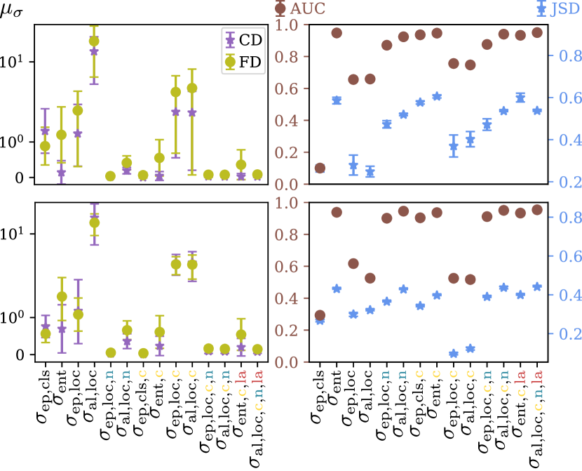
Despite the correlation between multiple types and failure cases, as discussed in Sec. 2, there exists a substantial overlap between of s and s (see the left of Fig. 3). The average () of s and s does not provide a clear indication of which type is optimal. We therefore consider the JSD and the AUC. Predicting on the validation set yields a ratio of 2% of s over s on KITTI and 31% on BDD. Particularly in such scenarios with imbalanced classes (s vs. s), Fig. 3 (right) highlights the advantage of JSD over AUC, as it captures distributional disparities between the distributions of s and s.
Fig. 3 (right) also demonstrates the importance of calibration for , particularly . However, normalizing by dividing it with the corresponding width and height of its bounding box enhances failure recognition rates the most. Consistent with prior work [Harakeh et al., 2020], proves to be a more discriminative uncertainty estimate for localization compared to , especially in noisy datasets. and perform best as separation candidates on both datasets. show comparable performance, with a deviation below 1%, to estimated using MC+LA. This suggests that the performance of non-epistemic uncertainties remains largely unaffected by dropout.
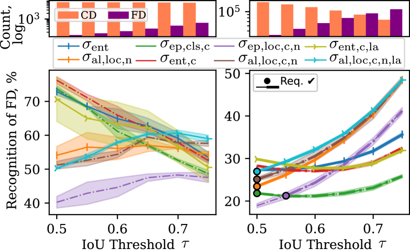
After comparing the separation capabilities of , we selectively retain the eight most promising candidates and discard the rest. The results of thresholding with an exemplary of s are presented in Fig. 4 to further analyze the behavior of each type. We observe that the defined criteria in Eqs. 2a and 2b are met at an IoU threshold of 0.8 for KITTI, but instead below 0.5 for BDD. This discrepancy can be attributed to the higher prevalence of s in BDD (see count in Fig. 4), making the exclusion of detections based on a valuable approach.
We notice that of an object detector with LA outperforms its MC+LA variant on both datasets, whereas does not. This can be attributed to the positive impact of LA on the quality of (see NLL in Tab. 2). Furthermore, Fig. 4 highlights the advantage of over the higher , since becomes more indicative of misdetections with stricter IoU requirements due to the independence of the classification error of . The performance of s consistently decreases on KITTI in contrast to s. Given the high performance of the object detector on KITTI and the few s, is more tailored to challenging cases in the dataset. As a result, it does not correlate with detections having relatively high IoU but still below , reducing the filtering efficiency as increases. As for calibration, it results in a recognition boost only up to a certain . This can be traced back to s with a lower IoU initially used for calibration now labeled as s based on the validation set, hence reducing the separation space between the of s and s.
4.3 Budget Behavior Analysis
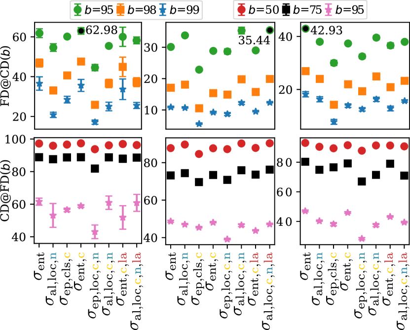
To assess the impact of the budget , Fig. 5 illustrates the introduced metrics in Eq. 4 for ranging from 0.5 to 0.99. Notably, increasing of s from 0.95 to 0.98 leads to an approximate 50% reduction in detected s across all datasets. However, increasing the detection of s by 25% results in only a 5–15% decrease in s. Recognizing the majority class (s) does not incur a significant error due to their abundance. However, when the focus shifts towards recognizing detections in the overlap region, the error begins to rise steeply. This emphasizes the challenges associated with accurately detecting instances that lie in the ambiguous overlap area illustrated in Fig. 3. plays a more significant role on BDD due to the lower localization performance, whereas on KITTI, dominates. The transferability of classification calibration models trained on BDD to CODA reveals that the difference in class characteristics between the two affects the effectiveness of , as performs best on CODA due to the lower classification performance (see Tab. 2). Overall, the suitability of the different types does not depend on the budget , but instead on the dataset and the challenges the model still faces at the end of training. While influences performance as expected, all types maintain it relatively to each other irrespective of .
4.4 Optimized Combined Thresholding
Given our results, we select to represent and to represent and . We include to continue the analysis on the usability of . We investigate the sum () and its optimization () of the selected types. We also explore their combination using multiplication and observe that the sum outperforms it. Tab. 3 demonstrates the benefits of optimization for the example of of s. It yields a 3–12% increase in FD@CD95 compared to using separate types (refer to Fig. 5) or combining them without optimization. without calibration or normalization results in only up to 15% FD@CD95 on KITTI and 2% on BDD.
Calibrating improves recognition rates on KITTI but not BDD/CODA due to the majority of detections used for calibration despite lower IoU thresholds, as also described in Sec. 4.2. However, whether using or , the increase in FD@CD95 of over falls within similar ranges. estimated via LA only and estimated via MC+LA also perform similarly (). Furthermoe, we observe that BAcc is not sufficiently descriptive, hence motivating the usage of our cost-sensitive evaluation metrics. For instance, BDD and CODA exhibit similar BAcc values despite notable differences in recognition rates. Nevertheless, optimization does result in an increase of up to 4% in BAcc. The only cost incurred by the optimization process is the 1–3 minutes average optimization time.
For further analysis, we optimize at both s 0.5 and 0.75 separately and notice that plays a smaller role (up to 8%) at higher s, while it contributes significantly more (up to a 20%) at lower s. carries nearly equal importance at both s. This behavior aligns with the outcomes depicted in LABEL:{fig:cdfdact}. Furthermore, is deemed redundant and assigned a weight of 0, as we assume that s are primarily caused by noisy images rather than a lack of images.
| Weights | FD@CD95 | BAcc | |||
|---|---|---|---|---|---|
| 1.000.00 | 1.000.00 | 1.000.00 | 68.021.97 | 0.810.01 | |
| 0.160.03 | 0.030.04 | 1.00.00 | 72.362.72 | 0.830.01 | |
| 1.000.00 | - | 1.000.00 | 65.863.43 | 0.800.02 | |
| 0.140.06 | - | 0.720.21 | 70.931.47 | 0.830.01 | |
| 1.000.00 | 1.000.00 | 1.000.00 | 32.030.24 | 0.630.00 | |
| 0.060.03 | 0.000.00 | 0.720.32 | 37.980.90 | 0.670.00 | |
| 1.000.00 | - | 1.000.00 | 30.650.23 | 0.630.00 | |
| 0.050.02 | - | 0.720.36 | 38.110.21 | 0.670.00 | |
| 1.000.00 | 1.000.00 | 1.000.00 | 40.600.21 | 0.680.00 | |
| 0.070.02 | 0.000.00 | 0.820.25 | 45.680.53 | 0.700.00 | |
| 1.000.00 | - | 1.000.00 | 38.490.96 | 0.670.00 | |
| 0.100.01 | - | 0.990.00 | 43.950.43 | 0.690.00 | |
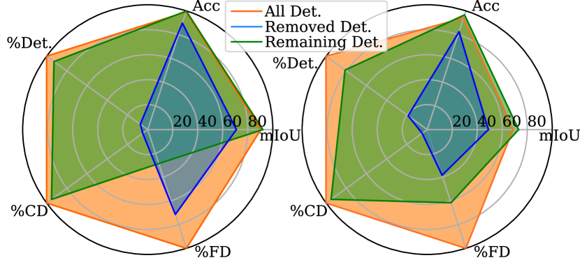
Discarding detections based on their uncertainty boosts the mIoU on average by up to 5% and Acc by 1.3% on BDD, with 18% removed detections (incl. 38% s and 5% s). On KITTI, discarding 7% (incl. 72% s and 4.95% s) increases the mIoU by up to 2% and the Acc by 0.7%. These findings visualized in Fig. 6 highlight the advantages of detecting more s (see count in Fig. 4), while emphasizing the necessity for a risk-aware evaluation. Overall, Fig. 6 illustrates the improvement in both the safety and performance of the detector via the substantial reduction of s via our approach while accepting an exemplary pre-defined budget of 5% loss of s.
5 Conclusion
We introduce a cost-sensitive, uncertainty-based, and optimized thresholding approach for failure recognition in object detection, allowing the detector to filter out its false detections during post-processing. We outline the requirements for effective thresholding, propose performance metrics for its evaluation, and investigate the challenges of uncertainty-based thresholding, including the role of epistemic and aleatoric uncertainties and their calibration. We find that a combination of softmax-based entropy and aleatoric uncertainty is optimal, hence avoiding epistemic uncertainty estimation methods and their computational drawbacks. Incorporating LA in a detector also reduces its inference time and enhances its performance. Our approach can remove 38–75% of s, at an exemplary cost of up to 5% increase in s, which is 3–12% more s compared to using separate calibrated and normalized uncertainties and 36–60% to using conventional methods, as in separate unprocessed uncertainties. We hope for this work to redirect the focus in object detection beyond performance to also include considerations of safety, without compromising either aspect.
References
- Appleyard and Yokim [2017] Jeremy Appleyard and Scott Yokim. Programming tensor cores in cuda 9. https://developer.nvidia.com/blog/programming-tensor-cores-cuda-9/, 2017. Accessed: 2023-6-26.
- Bahnsen et al. [2014] Alejandro Correa Bahnsen, Aleksandar Stojanovic, Djamila Aouada, and Björn Ottersten. Improving credit card fraud detection with calibrated probabilities. In SIAM International Conference on Data Mining, pages 677–685, 2014.
- Brodersen et al. [2010] Kay Henning Brodersen, Cheng Soon Ong, Klaas Enno Stephan, and Joachim M. Buhmann. The balanced accuracy and its posterior distribution. In 20th International Conference on Pattern Recognition, pages 3121–3124, 2010.
- Cai and Vasconcelos [2018] Zhaowei Cai and Nuno Vasconcelos. Cascade r-cnn: Delving into high quality object detection. In IEEE/CVF Conference on Computer Vision and Pattern Recognition, pages 6154–6162, 2018.
- Cheng et al. [2018] Bowen Cheng, Yunchao Wei, Rogerio Feris, Jinjun Xiong, Wen-mei Hwu, Thomas Huang, and Humphrey Shi. Decoupled classification refinement: Hard false positive suppression for object detection, 2018.
- Choi et al. [2021] Jiwoong Choi, Ismail Elezi, Hyuk-Jae Lee, Clement Farabet, and Jose M Alvarez. Active learning for deep object detection via probabilistic modeling. In IEEE/CVF International Conference on Computer Vision, pages 10264–10273, 2021.
- Corbière et al. [2019] Charles Corbière, Nicolas Thome, Avner Bar-Hen, Matthieu Cord, and Patrick Pérez. Addressing failure prediction by learning model confidence. Advances in Neural Information Processing Systems, 32, 2019.
- Cowen-Rivers et al. [2022] Alexander I Cowen-Rivers, Wenlong Lyu, Rasul Tutunov, Zhi Wang, Antoine Grosnit, Ryan Rhys Griffiths, Alexandre Max Maraval, Hao Jianye, Jun Wang, Jan Peters, et al. Hebo: pushing the limits of sample-efficient hyper-parameter optimisation. Journal of Artificial Intelligence Research, 74:1269–1349, 2022.
- Daftry et al. [2016] Shreyansh Daftry, Sam Zeng, J Andrew Bagnell, and Martial Hebert. Introspective perception: Learning to predict failures in vision systems. In IEEE/RSJ International Conference on Intelligent Robots and Systems, pages 1743–1750, 2016.
- DeVries and Taylor [2018] Terrance DeVries and Graham W Taylor. Learning confidence for out-of-distribution detection in neural networks, 2018.
- Fawcett [2006] Tom Fawcett. An introduction to roc analysis. Pattern recognition letters, 27(8):861–874, 2006.
- Gal and Ghahramani [2016] Yarin Gal and Zoubin Ghahramani. Dropout as a bayesian approximation: Representing model uncertainty in deep learning. In 33rd International Conference on Machine Learning, pages 1050–1059, 2016.
- Geifman and El-Yaniv [2017] Yonatan Geifman and Ran El-Yaniv. Selective classification for deep neural networks. Advances in Neural Information Processing Systems, 30, 2017.
- Geiger et al. [2012] A. Geiger, P. Lenz, and R. Urtasun. Are we ready for autonomous driving? The kitti vision benchmark suite. In IEEE/CVF Conference on Computer Vision and Pattern Recognition, pages 3354–3361, 2012.
- Google [2020] Google. GitHub - google/automl: Google Brain AutoML. https://github.com/google/automl, 2020. Accessed: 2023-08-02.
- Grimmett et al. [2013] Hugo Grimmett, Rohan Paul, Rudolph Triebel, and Ingmar Posner. Knowing when we don’t know: Introspective classification for mission-critical decision making. In IEEE International Conference on Robotics and Automation, pages 4531–4538, 2013.
- Guo et al. [2017] Chuan Guo, Geoff Pleiss, Yu Sun, and Kilian Q. Weinberger. On calibration of modern neural networks. In 34th International Conference on Machine Learning, page 1321–1330, 2017.
- Harakeh et al. [2020] Ali Harakeh, Michael Smart, and Steven L Waslander. Bayesod: A bayesian approach for uncertainty estimation in deep object detectors. In IEEE International Conference on Robotics and Automation, pages 87–93. IEEE, 2020.
- Hendrycks and Gimpel [2016] Dan Hendrycks and Kevin Gimpel. A baseline for detecting misclassified and out-of-distribution examples in neural networks, 2016.
- Kassem Sbeyti et al. [2023] Moussa Kassem Sbeyti, Michelle Karg, Christian Wirth, Azarm Nowzad, and Sahin Albayrak. Overcoming the limitations of localization uncertainty: Efficient and exact non-linear post-processing and calibration. In Machine Learning and Knowledge Discovery in Databases: Research Track. ECML PKDD 2023., pages 52–68. Springer Nature Switzerland, 2023.
- Kendall and Gal [2017] Alex Kendall and Yarin Gal. What uncertainties do we need in bayesian deep learning for computer vision? Advances in Neural Information Processing Systems, 30, 2017.
- Kuleshov et al. [2018] Volodymyr Kuleshov, Nathan Fenner, and Stefano Ermon. Accurate uncertainties for deep learning using calibrated regression. In 35th International Conference on Machine Learning, pages 2796–2804, 2018.
- Laves et al. [2021] Max-Heinrich Laves, Sontje Ihler, Jacob F. Fast, Lüder A. Kahrs, and Tobias Ortmaier. Recalibration of aleatoric and epistemic regression uncertainty in medical imaging, 2021.
- Le et al. [2018] Michael Truong Le, Frederik Diehl, Thomas Brunner, and Alois Knoll. Uncertainty estimation for deep neural object detectors in safety-critical applications. In 21st International Conference on Intelligent Transportation Systems, pages 3873–3878, 2018.
- Li et al. [2022] Kaican Li, Kai Chen, Haoyu Wang, Lanqing Hong, Chaoqiang Ye, Jianhua Han, Yukuai Chen, Wei Zhang, Chunjing Xu, Dit-Yan Yeung, Xiaodan Liang, Zhenguo Li, and Hang Xu. Coda: A real-world road corner case dataset for object detection in autonomous driving, 2022.
- Liang et al. [2017] Shiyu Liang, Yixuan Li, and Rayadurgam Srikant. Enhancing the reliability of out-of-distribution image detection in neural networks, 2017.
- Lin [1991] Jianhua Lin. Divergence measures based on the shannon entropy. IEEE Transactions on Information Theory, 37(1):145–151, 1991.
- Lin et al. [2014] Tsung-Yi Lin, Michael Maire, Serge Belongie, James Hays, Pietro Perona, Deva Ramanan, Piotr Dollár, and C Lawrence Zitnick. Microsoft coco: Common objects in context. In Computer Vision – ECCV 2014, pages 740–755, 2014.
- Miller et al. [2018] Dimity Miller, Lachlan Nicholson, Feras Dayoub, and Niko Sünderhauf. Dropout sampling for robust object detection in open-set conditions. In IEEE International Conference on Robotics and Automation, pages 3243–3249, 2018.
- Miller et al. [2019] Dimity Miller, Feras Dayoub, Michael Milford, and Niko Sünderhauf. Evaluating merging strategies for sampling-based uncertainty techniques in object detection. In IEEE International Conference on Robotics and Automation, pages 2348–2354, 2019.
- Rahman et al. [2019] Quazi Marufur Rahman, Niko Sünderhauf, and Feras Dayoub. Did you miss the sign? a false negative alarm system for traffic sign detectors. In IEEE/RSJ International Conference on Intelligent Robots and Systems, pages 3748–3753, 2019.
- Rahman et al. [2021] Quazi Marufur Rahman, Niko Sünderhauf, and Feras Dayoub. Online monitoring of object detection performance during deployment. In IEEE/RSJ International Conference on Intelligent Robots and Systems, pages 4839–4845, 2021.
- Saxena et al. [2017] Dhruv Mauria Saxena, Vince Kurtz, and Martial Hebert. Learning robust failure response for autonomous vision based flight. In IEEE International Conference on Robotics and Automation, pages 5824–5829, 2017.
- Sheng and Ling [2006] Victor S Sheng and Charles X Ling. Thresholding for making classifiers cost-sensitive. In 21st National Conference on Artificial Intelligence, pages 476–481, 2006.
- Stoycheva [2021] Mihaela Stoycheva. Uncertainty estimation in deep neural object detectors for autonomous driving. Master’s thesis, KTH, School of Electrical Engineering and Computer Science (EECS), 2021.
- Tan et al. [2020] Mingxing Tan, Ruoming Pang, and Quoc V. Le. Efficientdet: Scalable and efficient object detection. In IEEE/CVF Conference on Computer Vision and Pattern Recognition, pages 10778–10787, 2020.
- Thai-Nghe et al. [2010] Nguyen Thai-Nghe, Zeno Gantner, and Lars Schmidt-Thieme. Cost-sensitive learning methods for imbalanced data. In International Joint Conference on Neural Networks, pages 1–8, 2010.
- Tompson et al. [2015] Jonathan Tompson, Ross Goroshin, Arjun Jain, Yann LeCun, and Christoph Bregler. Efficient object localization using convolutional networks. In IEEE/CVF Conference on Computer Vision and Pattern Recognition, pages 648–656, 2015.
- Triebel et al. [2016] Rudolph Triebel, Hugo Grimmett, Rohan Paul, and Ingmar Posner. Driven learning for driving: How introspection improves semantic mapping. In 16th International Symposium of Robotics Research, pages 449–465, 2016.
- Yu et al. [2020] Fisher Yu, Haofeng Chen, Xin Wang, Wenqi Xian, Yingying Chen, Fangchen Liu, Vashisht Madhavan, and Trevor Darrell. Bdd100k: A diverse driving dataset for heterogeneous multitask learning. In IEEE/CVF Conference on Computer Vision and Pattern Recognition, pages 2633–2642, 2020.
- Zhang et al. [2014] Peng Zhang, Jiuling Wang, Ali Farhadi, Martial Hebert, and Devi Parikh. Predicting failures of vision systems. In IEEE/CVF Conference on Computer Vision and Pattern Recognition, pages 3566–3573, 2014.
- Zhang et al. [2023] Xu-Yao Zhang, Guo-Sen Xie, Xiuli Li, Tao Mei, and Cheng-Lin Liu. A survey on learning to reject. Proceedings of the IEEE, 111(2):185–215, 2023.