Indirect detection of dark matter absorption in the Galactic Center

Abstract

We consider the nuclear absorption of dark matter as an alternative to the typical indirect detection search channels of dark matter decay or annihilation. In this scenario, an atomic nucleus transitions to an excited state by absorbing a pseudoscalar dark matter particle and promptly emits a photon as it transitions back to its ground state. The nuclear excitation of carbon and oxygen in the Galactic Center would produce a discrete photon spectrum in the $\mathcal{O}(10)$ MeV range that could be detected by gamma-ray telescopes. Using the BIGSTICK large-scale shell-model code, we calculate the excitation energies of carbon and oxygen. We constrain the dark matter-nucleus coupling for current COMPTEL data, and provide projections for future experiments AMEGO-X, e-ASTROGAM, and GRAMS for dark matter masses from $\sim$ 10 to 30 MeV. We find the excitation process to be very sensitive to the dark matter mass and find that the future experiments considered would improve constraints on the dark matter-nucleus coupling within an order of magnitude.

I Introduction

Astrophysical systems are an excellent source for investigating dark matter (DM) interactions with the Standard Model (SM). Traditional indirect detection searches rely on observing the visible SM particles produced from DM annihilation or decay. As a consequence, DM-dominated systems such as dwarf spheroidal galaxies or the Galactic Center (GC) of the Milky Way provide ideal targets for such searches.

If DM is asymmetric [1] and stable, the standard annihilation and decay channels are not necessarily accessible to produce an indirect detection signal. There is, however, a broader theoretical landscape of DM models in which observable signals arise from DM processes beyond the standard paradigm [2]. For example, DM could be absorbed by (the nucleus of) an atom, resulting in (nuclear) atomic excitation and subsequent relaxation via emission of a monochromatic photon [3, 4]. Absorption of DM can also occur in semiconductors, resulting in multiphonon excitation [5]. In these works, the absorption of DM was considered in the context of direct detection and neutrino experiments.

In this work, we study a novel indirect detection signal arising from DM absorption by nuclei, resulting in nuclear line emissions that cannot be generated from known astrophysical processes. For example, line emissions generated from collisional excitations between interstellar gas/dust and cosmic rays, gamma ray emission due to neutron capture, or inverse Compton scattering [6, 7, 8] occur below $\sim$ 10 MeV [9, 10, 11, 7]. Since the absorption process involves both a DM particle and baryon, the high DM density and high baryon density environment of the GC is ideal for our indirect search.

The molecular gas in the inner Galaxy is rich in molecular hydrogen, helium, and carbon monoxide (CO) [12]. Of these components, CO is the most apt to study, because its abundance in the Galaxy is well-quantified through molecular transitions. Therefore, we focus on the nuclear excitation states of ^12C and ^16O, which we calculate using the BIGSTICK large-scale shell-model code [13, 14]. The excitation energies are on the order of 10 to 100 MeV, but we limit our scope to a maximum of $\sim$ 30 MeV, corresponding to the highest observed excitation state [15, 16].

We use COMPTEL data [17] to constrain our model for DM masses from $\sim$ 10 to 30 MeV, and we provide sensitivity projections for future experiments. COMPTEL observed gamma rays with energies from $\sim$ 1 to 30 MeV [18] and is the only existing gamma-ray data in the energy range of interest. Proposed future gamma ray telescopes such as AMEGO-X [19, 20], e-ASTROGAM [21], and GRAMS [22] would improve the sensitivity in the MeV regime. Therefore, we also provide sensitivity estimates for DM absorption with these experiments.

The organization of this paper is as follows. In Section II we describe the model of nuclear excitation via absorption of a pseudoscalar DM particle. In Section III we provide the velocity distribution functions and density profiles we use to model the DM halo and CO gas. In Section IV we show the calculation of the expected gamma ray flux from the nuclear de-excitation of ^12C and ^16O. In Section V we present and discuss our results for coupling constraints from COMPTEL data, as well as projections for future MeV gamma-ray experiments. We conclude in Section VI.

II Nuclear absorption

The nuclear absorption process can work for various types of DM particle, e.g., scalar, vector, pseudoscalar, axial vector, and fermion [4, 23, 24]. Here, we consider the nuclear excitation of a nucleus $n$ through the absorption of a pseudoscalar DM particle $\chi$,

$$n+\chi\rightarrow n^{*},$$ (1)

with interaction Lagrangian

$$\mathcal{L}=g_{\chi}Q_{b}(\partial_{\mu}\chi)\bar{q}\gamma^{\mu}\gamma^{5}q,$$ (2)

where $Q_{b}$ is the baryon number of quark species $q$ and $g_{\chi}$ is the DM-quark coupling constant (with dimension ${\rm energy}^{-1}$). The same bilinear quark term is also needed for axial vector DM interactions, while the $\bar{q}\gamma^{\mu}q$ and $\bar{q}q$ terms are needed for vector and scalar DM candidates. In this work, we do not consider any particular origin for DM, which can be model-dependent.

The absorption cross section in the center-of-mass frame is

$$\sigma^{\text{abs}}_{n\chi}(v_{\text{rel}}) =\frac{\pi}{6(2J_{n}+1)}g_{\chi}^{2}g_{A}^{2}S^{\text{GT}}\frac{|\vec{p}_{\chi}|^{2}}{v_{\text{rel}}}$$

$$\quad\times\frac{m_{n}+\Delta E}{E_{\chi}E_{n}}\delta(E_{\chi}+E_{n}-m_{n}-\Delta E),$$ (3)

where $J_{n}$ is the nuclear spin, $g_{A}=1.27$ is the axial form factor [25], $\vec{p}_{\chi}$ is the DM momentum, $v_{\text{rel}}\equiv\left|\vec{v}_{n}-\vec{v}_{\chi}\right|$ is the relative velocity between the DM particle and the nucleus, $E_{\chi}$ is the incident DM energy, $E_{n}$ is the initial energy of the nucleus, $m_{n}$ is mass of the nucleus, $\Delta E$ is the nuclear excitation energy, and

$$S^{\text{GT}}=|\langle\Phi_{f}||\sum_{i=1}^{A}\frac{1}{2}\hat{\sigma_{i}}\hat{\tau_{0}}||\Phi_{i}\rangle|^{2}$$ (4)

is the Gamow–Teller (GT) transition strength between the excited state $\Phi_{f}$ and ground state $\Phi_{i}$. Reference [26] shows that in the long-wavelength limit in which transfer momentum approaches zero, GT transitions are the dominant contribution to the total cross section among the multipole operators. Therefore, we approximate the DM absorption cross section by considering only the GT transition. For other types of DM (e.g., scalar, vector, axial vector), the GT transition might not dominate. Depending the spin and the parity of the DM and the nucleus, the dominant operator may be one of the following: electric monopole $\hat{\rho}$, electric dipole $\hat{d}$, magnetic moment $\hat{\mu}$, isovector spin dipole $\hat{D^{\sigma}}$, or spin $\hat{\sigma}$, which is equivalent to the GT operator.

We use the large-scale nuclear shell-model code BIGSTICK [13, 14] to calculate the nuclear excitation energy and corresponding GT transition strength in Eq. (4) of each ground-to-excited state transition for ^12C and ^16O. In BIGSTICK, we employ the YSOX interaction [27, 28], which is exactly diagonalized within the full $psd$ shell-model space ($0p_{1/2}$, $0p_{3/2}$, $0d_{5/2}$, $1d_{1/2}$, $0d_{3/2}$). The calculated GT strengths for each transition are shown in Fig. 1.

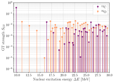
Figure 1: GT strengths for ^12C and ^16O, calculated using large-scale shell-model code BIGSTICK. Each line represents one excited state of the nucleus. Since de-excitation occurs directly to the ground state, the emitted photon energy is equal to the excitation energy $\Delta E$.

Nuclear excitation energies and strengths have also been measured in nuclear experiments. For example, the NDS database [29] collects nuclear data such as energy, transition type, and transition strength. Nevertheless, there are only a few GT transitions with documented energies and strengths, so the shell-model calculation is necessary in this study.

BIGSTICK is able to compute and produce excitation energies as high as $\mathcal{O}(100)$ MeV. However, for light nuclei such as ^12C and ^16O, the observed maximal excitation energy is $\sim 30$ MeV [15, 16]. Thus, we do not consider nuclear excitations above $\sim 30$ MeV.

III Galactic distribution functions

We assume a Navarro-Frenk-White (NFW) density profile for the Milky Way DM halo,

$$\rho(r)=\frac{\rho_{s}}{(r/r_{s})\left[1+(r/r_{s})\right]^{2}},$$ (5)

where $r$ is the radius from the GC, and the density and radial scales are fixed at $\rho_{s}=0.51~{}\text{GeV/}\text{cm}^{3}$ and $r_{s}=8.1~{}\text{kpc}$, respectively [30]. The CO gas density distribution is modeled using data from GALPROP v57 [31, 32] for galactic longitude $0.25^{\circ}\leq l\leq 359.75^{\circ}$ and latitude $|b|\leq 89.75^{\circ}$, each with $0.5^{\circ}$ bins. To calculate the CO mass density, we start with the CO intensity map (in units of K km s^-1) used in Ref. [33] and originally measured by Ref. [34]. To convert from intensity to number density, we use the mass conversion factor from CO to molecular hydrogen (H₂), $X_{\text{CO}}=2\times 10^{20}$ cm^-2 (K km s^-1)^-1 [33]. This then gives us the number density of H₂, which we assume is traced by the CO number density. The total gas mass of H₂ (CO) is given by Ref. [33] as $0.67\times 10^{9}M_{\odot}$ ($0.74\times 10^{9}M_{\odot}$). This provides us with a normalization factor to determine the CO mass density from the H₂ mass density, averaged per radial bin. Figure 2 shows the all-sky map of the CO column number density used for our analysis. In practice, we use the CO mass density for the remainder of our calculations.

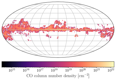
Figure 2: All-sky map of the column number density of CO used in our analysis. We assume the CO number density traces that of H₂, and calculate the H₂ number density from CO intensity maps provided in Ref. [33].

For the DM and nuclei $n\in\{\ce{{}^{12}C},\ce{{}^{16}O}\}$ velocities, we assume Maxwell-Boltzmann distributions of the form

$$f_{\chi}(r,\vec{v}_{\chi}) =\frac{\rho_{\chi}(r)}{(2\pi)^{3/2}(\sigma_{\chi}(r))^{3}}\text{e}^{-\vec{v}_{\chi}^{2}/2(\sigma_{\chi}(r))^{2}},$$ (6)

$$f_{n}(r,\vec{v}_{n}) =\frac{\rho_{n}(r)}{(2\pi)^{3/2}(\sigma_{n}(r))^{3}}\text{e}^{-(\vec{v}_{n}-\vec{v}_{\text{circ}}(r))^{2}/2(\sigma_{n}(r))^{2}},$$ (7)

where $\vec{v}_{\text{circ}}(r)$ is the circular baryon velocity, taken to be the rotation curve fit for $R_{\odot}=8.5~{}\text{kpc}$ from Ref. [35] (see Eq. (5) and Table 3). We note that more recent estimates find $R_{\odot}\approx 8.28~{}\text{kpc}$ [36].

The 1D velocity dispersions we use, in km/s, are given by

$$\sigma_{\chi}(r) \simeq\frac{1}{\sqrt{3}}\left(-43\ln{(r/r_{s})}+288\right),$$ (8)

$$\sigma_{n}(r) \simeq\begin{cases}-2.0\ln{(r/r_{s})}+3.3&r\leq r_{s}\\ 3.3&r>r_{s}.\end{cases}$$ (9)

We obtain the 1D DM velocity dispersion (which is related to the 3D velocity dispersion by $\sigma^{\text{1D}}=\sigma^{\text{3D}}/\sqrt{3}$) from a single fit to all of the 3D DM velocity dispersion profiles from the FIRE simulation results of Ref. [37] for $r\lesssim 50~{}\text{kpc}$. We fit the baryon velocity dispersion $\sigma_{n}(r)$ to the 1D CO-bright H₂ velocity dispersion of Ref. [38]. Since the baryon velocity dispersion from Ref. [38] only includes data to $r\sim 8.2~{}\text{kpc}$, we assume a constant $\sigma_{n}$ for $r>r_{s}$.

We normalize the velocity distribution functions such that

$$\int_{0}^{v_{\text{esc}}(r)}d^{3}v_{\chi}~{}f_{\chi}(r,\vec{v}_{\chi}) =\rho_{\chi}(r),$$ (10)

$$\int_{0}^{v_{\text{esc}}(r)}d^{3}v_{n}~{}f_{n}(r,\vec{v}_{n}) =\rho_{n}(r),$$ (11)

where the escape velocity of the Milky Way is taken to be $v_{\text{esc}}(r)=\sqrt{2}v_{\text{circ}}(r)$. We note that this relation underestimates the escape velocity compared to recent estimates based on Gaia DR2 [39, 40], Gaia DR3 [41], and the RAVE survey [42].

IV Photon flux

For a DM particle absorbed by nucleus $n$, the photon spectrum from the de-excitation of the nucleus is

$$\frac{dN^{n\chi}}{dE_{\gamma}}=\delta(\Delta E-E_{\gamma}),$$ (12)

where $E_{\gamma}$ is the true photon energy. The differential flux or intensity (in units of cm^-2 s^-1 sr^-1 MeV^-1) of the resulting de-excitation photon is

$$\frac{d^{2}\Phi}{dE_{\gamma}d\Omega} =\frac{1}{4\pi}\frac{dN^{n\chi}}{dE_{\gamma}}\int ds\int d^{3}v_{n}\frac{f_{n}(r(s,\psi),\vec{v}_{n})}{m_{n}}\int d^{3}v_{\chi}\frac{f_{\chi}(r(s,\psi),\vec{v}_{\chi})}{m_{\chi}}\sigma^{\text{abs}}_{n\chi}(v_{\text{rel}})v_{\text{rel}},$$ (13)

where $s$ is the line-of-sight distance, $\psi$ is the angle between the line of sight and the line from the point of observation (taken to be our Sun) to the center of the Milky Way halo, and $m_{\chi}$ is the DM mass.

Working in the non-relativistic limit $(p_{\chi}=m_{\chi}v_{\chi})$, we write the delta function in Eq. (II) in terms of $v_{\chi}$ to obtain

$$\sigma^{\text{abs}}_{n\chi}(v_{\text{rel}}) =\frac{\pi}{6(2J_{n}+1)}g_{\chi}^{2}g_{A}^{2}S^{\text{GT}}\frac{|\vec{p}_{\chi}|^{2}}{v_{\text{rel}}}$$

$$\quad\times\frac{m_{n}+\Delta E}{E_{\chi}E_{n}}\frac{\delta(v_{\chi}-v_{\chi}^{+})}{m_{\chi}v_{\chi}^{+}},$$ (14)

where

$$v_{\chi}^{+}=\sqrt{\frac{2(\Delta E-m_{\chi}-\frac{1}{2}m_{n}v_{n}^{2})}{m_{\chi}}}.$$ (15)

Since the numerator under the square root must be positive and $v_{\chi}^{+}<v_{\text{esc}}$, the bounds on the baryon velocity distribution integral in Eq. (11) become

$$\sqrt{\frac{2(\Delta E-m_{\chi}-\frac{1}{2}m_{\chi}v_{\text{esc}}^{2})}{m_{n}}}\leq v_{n}\leq\sqrt{\frac{2(\Delta E-m_{\chi})}{m_{n}}}.$$ (16)

The kinematics of the nuclear excitation process are extremely sensitive to $m_{\chi}$ such that to achieve a nonzero photon flux, the values of $\Delta E$ and $m_{\chi}$ must be very close to one another. For DM velocity $v_{\chi}^{+}$ bounded by $v_{\text{esc}}\approx 10^{-3}$, the difference between $\Delta E$ and $m_{\chi}$ is maximized when $v_{n}=0$, for which Eq. (15) gives $(\Delta E/m_{\chi}-1)\lesssim 5\times 10^{-7}$.

The line-of-sight integral is from the location of the detector at $s=0$ to the source location at

$$s=\sqrt{R_{\text{halo}}^{2}-R_{\odot}^{2}\sin^{2}\psi}+R_{\odot}\cos\psi,$$ (17)

where $R_{\text{halo}}=50~{}\text{kpc}$ is the maximum galactocentric radius considered. The galactocentric radial coordinate $r$ is related to the line-of-sight distance $s$ by

$$r(s,\psi)=\sqrt{R_{\odot}^{2}+s^{2}-2R_{\odot}s\cos\psi},$$ (18)

where $\psi$ is related to galactic longitude and latitude by $\cos\psi=\cos{l}\cos{b}$.

V Current constraints and future projections

To determine constraints on the DM-nucleus coupling $g_{\chi}$, we numerically calculate the theoretical differential flux in Eq. (13) for each nuclear excitation energy $\Delta E$ of $\ce{{}^{12}C}$ and $\ce{{}^{16}O}$ and for a range of DM masses. For each $\Delta E$, there is only a narrow range of DM masses $m_{\chi}~{}\in~{}[E_{\gamma}-10^{-2}~{}\text{MeV},~{}E_{\gamma})$ that give a non-zero differential flux, due to the kinematics of the interaction requiring that

$$\Delta E=m_{\chi}+\frac{1}{2}m_{\chi}v_{\chi}^{2}+\frac{1}{2}m_{n}v_{n}^{2}.$$ (19)

To approximate the observed spectrum at the detector, the true photon spectrum in Eq. (12) is convolved with a Gaussian distribution. For an experiment with energy resolution $\epsilon E_{\gamma}$, the probability of observing a photon of energy $E$ from a gamma ray of true energy $E_{\gamma}$ is [43]

$$R_{\epsilon}(E-E_{\gamma})\approx\frac{1}{\sqrt{2\pi\epsilon^{2}E_{\gamma}^{2}}}\exp\left[-\frac{(E-E_{\gamma})^{2}}{2\epsilon^{2}E_{\gamma}^{2}}\right].$$ (20)

The energy resolutions for the experiments we consider are listed in Table 1.

V.1 Constraints from COMPTEL data

Intensity maps for the inner galactic plane were calculated by Ref. [44] using COMPTEL observations for 1–3 MeV, 3–10 MeV, and 10–30 MeV energy bins over the angular range $330.0^{\circ}\leq l\leq 359.0^{\circ},0.5^{\circ}\leq l\leq 30.0^{\circ}$ and $|b|\leq 5^{\circ}$. We fit the upper and lower limits of the $E^{2}\times\text{intensity}$ COMPTEL results to a piecewise linear function over each energy bin (see Fig. 3 of Ref. [44]) and integrate the fitted function over each energy bin. We use this information to compare with the prediction from DM absorption: after we integrate over the same angular range as the COMPTEL data and divide by solid angle, we convolve the differential flux in Eq. (13) with Eq. (20). We then multiply by $E^{2}$ and integrate over the relevant energy bin, using an energy resolution of $\epsilon=2\%$. While Ref. [44] used binning of $1^{\circ}$ for $l$ and $5^{\circ}$ for $b$, we use $0.25^{\circ}$ bins for both $l$ and $b$. Since our baryon density data ranges from $0.25^{\circ}\leq l\leq 359.75^{\circ}$ and $|b|\leq 89.75^{\circ}$ in $0.5^{\circ}$ bins, using $0.25^{\circ}$ bins allows us to match the same angular range, as well as use all CO density data points in the range we consider. For intermediate values of $l$ and $b$ we use linear interpolation to determine the CO density.

We use COMPTEL data to calculate constraints on $g_{\chi}$ by insisting that the prediction of $\int dE\,E^{2}\times\text{intensity}$ from the DM absorption process cannot exceed the observation within the appropriate energy bin. Our results are shown in Fig. 3 for a single $\ce{{}^{12}C}$ excitation energy and in Fig. 4 for all $\ce{{}^{12}C}$ and $\ce{{}^{16}O}$ excitation energies up to 30 MeV. The absorption process and thus the intensity spectra are very sensitive to $m_{\chi}$; therefore, results are sharply peaked near the nuclear de-excitation energy, approximating a delta function centered at

$$m_{\chi}\approx\Delta E-\frac{1}{2}m_{n}v_{n}^{2}$$ (21)

with $v_{n}\approx 219~{}\text{km/s}$. The extreme sensitivity to the DM mass means that despite $\ce{{}^{12}C}$ and $\ce{{}^{16}O}$ excitation energies that appear to be very close to one another in Fig. 1, we find that any DM mass that results in a nuclear excitation only excites a single energy transition.

Experiment	Energy range	Energy resolution $\mathbf{\epsilon}$
COMPTEL [17]	0.75 - 30 MeV	2-4% (5-10% FWHM)
AMEGO-X [20]	25 keV - 1 GeV	2% (5% FWHM) at 1 MeV
e-ASTROGAM [45]	30 keV - 200 MeV	3.0% at 1 MeV
GRAMS [46]	0.2 MeV - 100 MeV	1% at 2.5 MeV

Table 1: Energy resolutions for each experiment considered in our analysis. For COMPTEL, we use the smallest energy resolution of 2%. For COMPTEL and AMEGO-X, we calculate $\epsilon$ from $\epsilon~{}=~{}\text{FWHM}/(2\sqrt{2\ln 2})$. The GRAMS energy resolution of 1% is estimated from the nEXO experiment (see Ref. [46]).

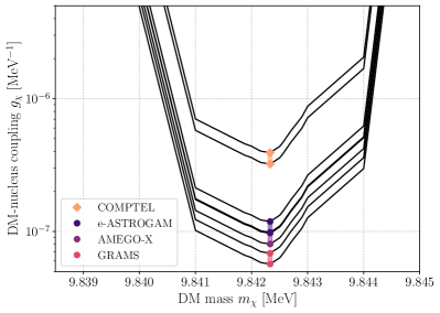
Figure 3: Upper limit constraints on $g_{\chi}$ for DM absorption by $\ce{{}^{12}C}$ for a single excitation energy, $\Delta E~{}\approx~{}9.845$ MeV, for DM masses that give a non-zero differential flux. Two points of the same color represent the upper and lower uncertainties on $g_{\chi}$ for a given experiment, determined by the data presented in Ref. [44]. For this excitation energy, COMPTEL limits are derived by integrating over the 3–10 MeV energy bin. For future experiments e-ASTROGAM, AMEGO-X, and GRAMS, these limits represent 68% confidence level as the convolved spectrum is integrated over the range $E_{\gamma}\pm\epsilon E_{\gamma}$. The constraint points are drawn only at the lowest point of the DM mass curve, i.e. at the most constraining DM mass for this nuclear excitation energy, which corresponds to a baryon velocity of $v_{n}\approx 219~{}\text{km/s}$ from Eq. (21). Note that AMEGO-X’s upper limit point overlaps with the lower limit point of e-ASTROGAM, and is therefore not visible in the figure.

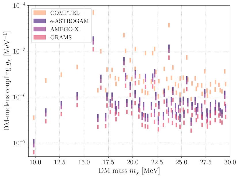
Figure 4: Upper limit constraints on $g_{\chi}$ for DM absorption by $\ce{{}^{12}C}$ and $\ce{{}^{16}O}$, derived from existing COMPTEL data from Ref. [44] (with assumed energy resolution for COMPTEL of $\epsilon=2\%$), and projected constraints for future experiments e-ASTROGAM [45] (assumed energy resolution of $\epsilon=3\%$), AMEGO-X [20] ($\epsilon=2\%$), and GRAMS [46] ($\epsilon=1\%$). Each shaded rectangle represents the possible values of $g_{\chi}$ for each $\ce{{}^{12}C}$ or $\ce{{}^{16}O}$ excitation energy shown in Fig. 1, with upper and lower uncertainties determined by the data presented in Ref. [44]. As in Fig. 3, the constraints shown are from the most constraining DM mass for each nuclear excitation energy. The photon flux is found to be very sensitive to the value of $m_{\chi}$ such that the range of DM masses that will result in the excitation of the nucleus for a particular excitation energy $\Delta E$ is very narrow, as shown in Fig. 3 for a single $\ce{{}^{12}C}$ excitation energy. Here we omit the black line in Fig. 3 for clarity, which in this plot would appear as a vertical line.

V.2 Projections for future experiments

As a proxy for the data observed by future experiments, we fit the COMPTEL data from Ref. [44] to a smooth function over the full 1–30 MeV energy range for the upper and lower COMPTEL uncertainty bands to obtain

$$E^{2}\times\text{intensity}$$ (22)

$$=\begin{cases}(1.5\times 10^{-3})\ln\left(\frac{\text{E}}{\text{MeV}}\right)+(1.2\times 10^{-2})&\text{lower}\\ (2.4\times 10^{-3})\ln\left(\frac{\text{E}}{\text{MeV}}\right)+(1.7\times 10^{-2})&\text{upper},\end{cases}$$

in units of MeV cm^-2 s^-1 sr^-1. We assume idealized optimal energy bins, with each bin centered on the de-excitation photon energy $E_{\gamma}$ and with width $E_{\gamma}\pm\epsilon E_{\gamma}$. The differential flux in Eq. (13) is integrated and averaged the over the same angular range used in Section V.1.

We consider future experiments AMEGO-X, e-ASTROGAM, and GRAMS, and use the smallest $\epsilon$ provided by their respective references at the energies most relevant to our study, listed in Table 1. Following the same procedure as in Section V.1, we integrate over the energy range $E_{\gamma}\pm\epsilon E_{\gamma}$. Our results are shown in Fig. 3 for a single $\ce{{}^{12}C}$ excitation energy and in Fig. 4 for all $\ce{{}^{12}C}$ and $\ce{{}^{16}O}$ excitation energies.

Of the future experiments considered, e-ASTROGAM is the least constraining on $g_{\chi}$, having the largest expected energy resolution at $3\%$, while GRAMS is the most constraining with the best expected energy resolution of 1%. Comparing current COMPTEL data to projected sensitivities, limits on $g_{\chi}$ improve by almost an order of magnitude on average, but we note that these projections are optimistic because of the optimized energy binning that we use. Even though COMPTEL’s energy resolution of $2\%$ is the same as that of AMEGO-X, COMPTEL is much less constraining due to the large energy bins.

Current constraints on the on the $g_{\chi}$ vs $m_{\chi}$ parameter space exist in the context of axion-like particles (ALPs) coupled to nucleons and emitted from stars and from supernova (SN) cores [47]. The solar ALP flux search at the Sudbury Neutrino Observatory excludes $g_{\chi}\gtrsim 2\times 10^{-8}~{}\text{MeV}^{-1}$ for $m_{\chi}\lesssim 2~{}\text{MeV}$, while the SN 1987A cooling constraint excludes $3\times 10^{-13}$ MeV${}^{-1}\lesssim g_{\chi}\lesssim 2\times 10^{-9}$ MeV^-1 for DM masses $m_{\chi}\lesssim 100$ MeV, where we have related the DM-nucleon coupling constant $g_{\chi}$ to the DM-proton $p$ coupling $g_{ap}$ of Ref. [47] by $g_{\chi}=g_{ap}/2m_{p}$, where $m_{p}$ is the mass of the proton.

VI Conclusion

In this work we consider the absorption of a pseudoscalar DM particle by a nucleus, resulting in nuclear excitation and the subsequent release of a photon. For $\ce{{}^{12}C}$ and $\ce{{}^{16}O}$ present in the GC, we use the BIGSTICK large-scale shell-model code to calculate nuclear excitation levels from $\sim$ 10 to 30 MeV, energies detectable by gamma-ray experiments. Using current COMPTEL data, we constrain the DM-nucleus coupling and provide projections for future experiments AMEGO-X, e-ASTROGAM, and GRAMS.

We find this nuclear excitation process to be extremely sensitive to the DM mass due to the narrow-width approximation of the absorption. Relaxing this approximation would produce smoother limits, though still peaked at the same DM masses.

For the model considered, we estimate future experiments would improve constraints on the DM-nucleus coupling by almost an order of magnitude compared to current data. We expect constraints on other types of DM particle to be within one order of magnitude of these results, since they differ only by the degree of freedom of the DM spin. For example, the cross section of fermionic DM is $\sim 2$ times higher than that of scalar/pseudoscalar DM.

With new proposed telescopes such as AMEGO-X, e-ASTROGAM, GRAMS, and others such as COSI [48] (expected to launch in 2027), and GECCO [49], sensitivity in the MeV range is expected to improve significantly, bridging the gap between hard X-ray and soft gamma-ray astronomy. In particular, AMEGO-X, e-ASTROGAM, and GRAMS would provide unprecedented sensitivity to both MeV-scale line emissions and continuum emission, improving upon COMPTEL’s sensitivity by several orders of magnitude. Such experiments would provide insight into the origin of the MeV continuum emission, in addition to improving sensitivity to indirect detection signals.