Lens Stochastic Diffraction:
A Signature of Compact Structures in Gravitational-Wave Data
Abstract
Every signal propagating through the universe is diffracted by the gravitational fields of intervening objects, aka gravitational lenses. Diffraction is most efficient when caused by compact lenses, which invariably produce additional images of a source. The signals associated with additional images are generically faint, but their collective effect may be detectable with coherent sources, such as gravitational waves (GWs), where both amplitude and phase are measured. Here, I describe lens stochastic diffraction (LSD): Poisson-distributed fluctuations after GW events caused by compact lenses. The amplitude and temporal distribution of these signals encode crucial information about the mass and abundance of compact lenses. Through the collective stochastic signal, LSD offers an order-of-magnitude improvement over single lens analysis for objects with mass . This gain can improve limits on compact dark-matter halos and allows next-generation instruments to detect supermassive black holes, given the abundance inferred from quasar luminosity studies.
I Introduction
Gravitational lensing, the deflection of propagating signals by intervening gravitational fields, is a sensitive probe of matter distribution. It illuminates the Universe’s darkest objects: black holes [1, 2, 3, 4] and dark matter halos [5, 6, 7, 8, 9, 10]. Most lensing applications to date rely on electromagnetic sources. However, the emergence of gravitational wave (GW) astronomy [11, 12, 13, 14, 15, 16] provides new opportunities for gravitational lensing, which motivate detection strategies [17, 18, 19, 20, 21, 22]. Given the steady improve in sensitivity, multiply imaged GW sources are bound to become a reality in the near future [23, 24, 25, 26, 27]. The detection of lensed GWs will provide new applications in cosmology, astrophysics and fundamental physics [28, 29, 30, 31, 32], including the detection and characterization of dark-matter structures [33, 34, 35, 36, 37, 38, 39, 40, 41, 42, 43, 44, 45, 46, 47].
GW lensing is highly complementary to lensed electromagnetic radiation [48, 49, 50]. As GW detectors are sensitive to field amplitude and phase (rather than energy flux), the signal strength decreases with distance (rather than distance squared), facilitating the detection of remote sources. In lensing, this scaling makes GWs more robust to demagnification, allowing the observation of faint images, including strongly deflected trajectories for sources near a massive black hole [51, 52, 53], central images of strongly lensed systems [35, 54], and systems with large lens-source angular separation [28, 55, 56, 57, 47, 58]. The prospects of observing faint images increases significantly because the number of lenses scales with the square of source-lens separation.
In addition to loud transient signals, detectors are also sensitive to GW backgrounds, a stochastic superposition of many faint signals. An astrophysical background from unresolved mergers is expected [59], and cosmological backgrounds could be produced by early-universe phenomena [60]. Although signals are too weak to be resolved, their existence can be inferred as an excess over instrumental noise, or by cross-correlating the output of multiple detectors [61, 62, 63].
Here, I present lens stochastic diffraction (LSD), a novel signature of compact structures consisting of faint counterparts present after loud GW events. These secondary signals, caused by compact lenses, follow a stochastic distribution, resembling that of GW backgrounds. I will introduce the LSD signal caused by an ensemble of point lenses, derive its time distribution and signal-to-noise ratio, and show its potential to detect compact objects, before discussing open issues and prospects.
II Lens stochastic diffraction
A point-like gravitational lens forms at least one additional image of any source. The ratio of the lensed/unlensed flux is given by the magnification, which for an isolated point lens reads
| (1) |
Here labels the main/additional image and the sign corresponds to the parity. is the image-lens angular separation: coordinates are centered around the undeflected source and , are the image and lens position in units of the Einstein angle, . The angular diameter distances , , (for observer-lens observer-source and lens-source, respectively) are given by flat-CDM cosmology [64].
The existence of a faint image near the lens is associated with a strongly deflected trajectory. At large angular separations, , the secondary image flux scales as . In typical electromagnetic sources, strong demagnification prevents the observation of additional images in generic source-lens configurations. Instead, the signal amplitude of GWs is modulated by , making faint images more easily observable.
Increasing the offset decreases the amplitude of individual images but increases their number: N point lenses produce at least images and as many as [65].111Even more images form when lenses are distributed at different distances, because of consecutive deflections. I will neglect those and assume that all lenses can be projected onto a common lens plane by rescaling the Einstein radii [66]. The enclosed average number of lenses
| (2) |
depends on the line of sight via the convergence , where the projected surface density of compact objects. The lens number follows a Poisson distribution , with set by the line of sight to the source. The average convergence is [67]
| (3) |
where is the Hubble constant and is the fraction of compact objects, relative to the dark-matter abundance and the comoving density of compact objects is assumed constant. For point lenses is independent of the lens’ mass.
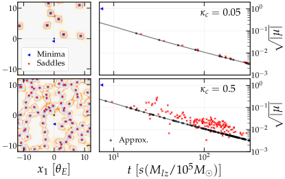
Scaling with suggests that secondary images will rarely be identified individually but can be detected collectively. Fig. 1 shows the distributions of images in the sky and their amplitude and delay, for two realizations with low and high . The results are obtained from numerical solutions and assuming isolated lenses, Eq. (1). For at most one lens is closely aligned with the source. Then Eq. (1) describes the two brightest images, plus other secondary images with . The higher increases both individual magnifications and the chance of forming additional images [68, 69, 70]. Therefore, the isolated lens approximation is accurate for and conservative otherwise (see Fig. 3 below). Hereafter I assume that lenses can be treated as isolated.
The time distribution of secondary images encodes information about the lens mass distribution. Each secondary image arrives with a characteristic delay, which depends on the lens mass, redshift and offset as
| (4) |
where the second equality defines a dimensionless delay. To remain in the geometric optics description, we will require that the time delays between different images satisfy , where is the GW frequency [50].
A GW signal lensed by a collection of point-particles in the geometric optics regime is described by
| (5) |
Here is the primary image magnification, not directly observable, and includes the detector antenna pattern. The index labels the additional images and is the Hilbert-transform of the unlensed signal, accounting for the phase difference in negative parity images [71, 72].222 Positive parity images can be included in Eq. (5) by adding , where index secondary minima and maxima of the time delay, respectively. Under the sparsity assumption there is one image per lens and is well approximated by Eq. (1)
The lens stochastic diffraction (LSD) signal is defined by the sum of additional images in Eq. (5). Although stochastic, it differs from GW backgrounds:
-
1.
LSD is neither stationary nor Gaussian: its correlation with the primary GW signals is determined by the lens mass distribution (Eq. 4).
-
2.
Although most GW backgrounds are isotropic, the LSD is received from the same sky localization as the main signal.
-
3.
The waveform of individual LSD contributions is known from the resolved signal (Eq. 5), up to parameter-estimation uncertainties.
LSD also differs from the contribution on the astrophysical stochastic background from magnified high redshift sources [73, 74, 75].
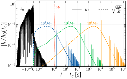
Examples of LSD realizations following an equal-mass, non-spinning merger are shown in Fig. 2 for different lens masses. The projected density corresponds to a source at with .
III Temporal distribution and signal-to-noise ratio
Let us now investigate the temporal distribution and signal-to-noise ratio (SNR) of LSD. To separate LSD in Eq. (5), I will introduce a window function that is one for s after coalescence and zero elsewhere (Fig. 2). The LSD signal is .
The SNR of the LSD after a GW event is then , where is the noise-weighted inner product [76]. The LSD-SNR is
| (6) |
where is the SNR of the unlensed event and is the match between different images. The first sum in Eq. (6) represents the contribution of each image after . The double sum accounts for interference between separate images and has zero average, since ’s are not correlated. Eq. (6) assumes a constant antenna pattern, a good approximation for d, or .333For large the average LSD-SNR will beslightly lower due to selection bias, as a detection threshold favors events with .
Let us now study the average LSD-SNR relative to the unlensed event, . The sum over images is replaced by integrals weighted by the lens number density . Assuming isolated lenses, the average relative differential LSD-SNR is
| (7) |
Here is the derivative of Eq. (3), is the lens mass function and the average lens density has been used (Eq. 2). The magnification and time delay are evaluated as for an isolated lens, cf. Eqs. (1,4).
The total LSD-SNR is the integral of Eq. (7) over time and lens mass. If it simplifies to
| (8) |
Note that including will add a dependence on both the lens’ mass and the source redshift, which is important for (cf. Fig. 2). Similarly, an upper limit on the time delays considered needs to be included, which will affect the sensitivity to high mass objects.
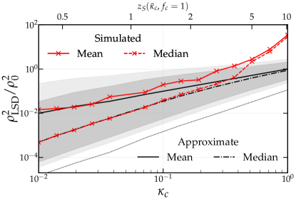
The distribution of the LSD-SNR depends strongly on , whose summary statistics are shown in Fig. 3. For the isolated lens approximation, the mean of random realizations agrees with Eq. (8). At low , the distribution is skewed, as the median deviates from the mean due to rare events with high (). The LSD-SNR distribution was obtained numerically, using Eq. (6) (only first sum) for random realizations at each value of . The simulated LSD-SNR becomes larger than the approximate value of due to the formation of additional images and collective lensing effects, confirming that the isolated lens approximation is conservative.
IV Observational prospects
Let us now estimate the sensitivity of ground detectors to LSD given the abundance of compact objects, . The rate calculation follows Refs. [77, 78]. I consider the LIGO-Virgo-KAGRA (LVK) detector network at O5 sensitivity, the Einstein Telescope (ET) [79] and a single Cosmic Explorer (CE) interferometer [80]. I will consider only non-spinning and quasicircular black hole mergers.
The detection rate and the average LSD-SNR for source catalogue are given by
| (9) | ||||
| (10) |
Here are the binary intrinsic parameters and is the population model given by the “power law + peak” model (fiducial parameters in Ref. [81]). The volume element, is that of flat CDM [64] and the source distribution, , follows the star formation rate [82], with a normalization [83]. is the fraction of detected sources, which depends on the ratio of the detection threshold to the optimal SNR , with . and are obtained using gwfast [84, 85]. The LSD-SNR depends on the second moment and .
The mass of the lens affects the total LSD-SNR by changing the arrival time of secondary signals (Eq. 4) relative to in the window function. Eq. (10) is valid for : The effect of is estimated by multiplying by (Eq. 7), assuming (below the typical source redshfit for future detectors). Note that LSD includes lensed events where secondary signals are individually detected, .
Detection of the LSD or its absence provides competitive limits on the abundance of compact objects with . Fig. 4 shows current lensing constraints from quasars [86], stars [87, 88, 89], type Ia supernovae [90] and GWs from LVK O3a [38], as well as expected limits from fast radio bursts (FRBs) [91], GWs under single-lens analysis [39, 40] and with LSD (90% c.l. and 1 year of observation). The lensing limits for will be dominated by lensed GWs in the near future. Single-lens analyzes are more constraining for objects with . The improvement is due to wave-optics lensing effects, which are excluded from the LSD by signal windowing. Instead, for , LSD incorporates information from low-amplitude images, representing an order-of-magnitude gain in sensitivity.
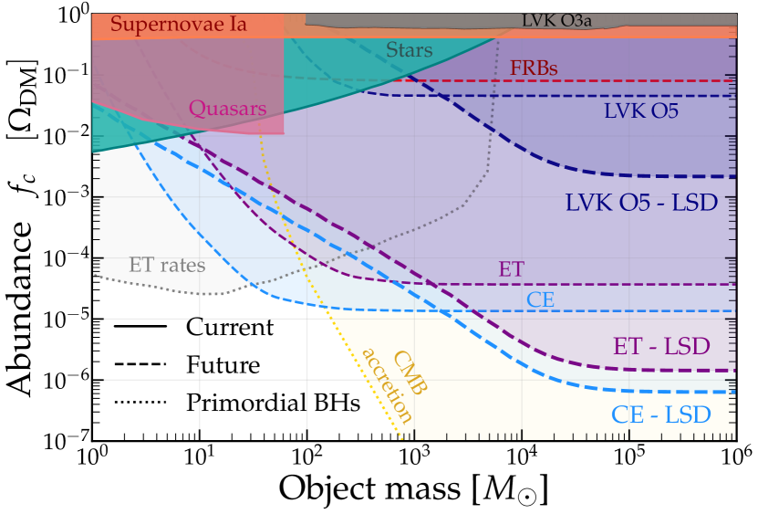
LSD constraints are complementary to other probes of compact objects and dark matter. For comparison, Fig. 4 shows two model-dependent limits for primordial black holes: current cosmic microwave background (CMB) accretion limits [92] and forecasted limits from merger rate by ET [93]. Although stringent, these limits require dark matter to be very compact and be present before recombination. In contrast, LSD probes extended structures, such as compact dark-matter halos and black holes of astrophysical origin. Then, the finite size prevents the formation of additional images for offsets , where is the object’s size over its Einstein radius. This allows objects with to be probed by LSD, times larger than the CMB [94]. The effect of lens size can be determined accurately by changing in Eq. (7).444A cutoff for secondary images in causes a drop in the LSD after a characteristic delay (Eq. 4), whose observation can constrain the lens properties. Non-singular lenses also form central images [35], whose short time delay may introduce wave-optics distortions. The analysis here can be extended by replacing with the distorted waveform from the extended lens.
Two potential targets of LSD are supermassive black holes (SMBHs) and compact dark-matter halos. Both ET and CE have the potential to probe SMBHs via LSD, with estimated from the quasar luminosity function [95, 96]. Other systems, such as lensed gamma-ray bursts, suggest the existence of compact lenses whose mass and abundance could be further probed by LSD [97, 98, 99]. Beyond detection, the temporal distribution of the LSD (Eq. 7) can be used to constrain the mass function of compact structures.
V Discussion
Lens stochastic diffraction (LSD) is a new signature of compact lenses in GW data, sensitive to objects with . After a GW event, it manifests itself as multiple secondary signals, each a phase-shifted faint copy of the main event (Figs. 1,2). The delays follow a Poisson distribution, depending on the object’s mass and abundance. Secondary signals can only be individually identified if a lens is closely aligned with the source. However, considering these signals collectively enables LSD to effectively probe compact objects.
LSD can detect compact lenses more efficiently than single lens analysis of GWs and electromagnetic transients for (Fig. 4). While the CMB is a more powerful test of primordial black holes, LSD is sensitive compact dark-matter halos and objects formed after recombination. It complements existing methods [100, 94, 101] and can target specific theories, such as compact axion structures [102]. Beyond ground GW interferometers, space detectors like LISA [103, 104] can leverage the high SNR and redshift of massive black hole mergers.
Several challenges must be addressed to extract the LSD signature from real data. Uncertainties in the main signal (from parameter estimation, differences in the lens model) will degrade the SNR by the mismatch between the true and assumed waveforms. Astrophysical GW backgrounds provide a source of confusion with LDS signals. Among the unresolved events, some will have intrinsic parameters and sky localization similar enough to the main signal to be confused with LSD (analogous to the issue of false alarm probability in strongly imaged events [26, 105]). The LSD can be distinguished by exploiting the correlation with resolved signals, which are absent in stochastic backgrounds. Further improvements are expected by incorporating techniques for stochastic backgrounds that leverage waveform information [106, 107, 108, 109]. These methods will alleviate the impact of data glitches and contamination from GW backgrounds.
LSD has interesting connections to strong lensing and microlensing. The time distribution of secondary images (whether they appear after, around, or before the primary signal) could be used to reveal the image type [110, 111]. Most interestingly, extending the analysis to the wave-optics regime will provide insights into lighter lenses, including signatures of stars in multiply imaged GWs [112, 113, 114, 115, 116, 117, 118, 119, 120].
Acknowledgements.
I am very grateful to S. Goyal, S. Savastano and H. Villarrubia-Rojo for comments on the manuscript, to G. Brando, J. Gair, G. Tambalo and Y. Wang for discussions and Han Gil Choi also for sharing the results of Ref. [40]. This work relied on Gwfast [84, 85], PBHbounds [121], Astropy [122, 123, 124], Numpy [125] and Scipy [126].References
- Sahu et al. [2022] K. C. Sahu et al. (OGLE, MOA, PLANET, FUN, MiNDSTEp Consortium, RoboNet), An Isolated Stellar-mass Black Hole Detected through Astrometric Microlensing, Astrophys. J. 933, 83 (2022), arXiv:2201.13296 [astro-ph.SR] .
- Lam et al. [2022] C. Y. Lam et al., An Isolated Mass-gap Black Hole or Neutron Star Detected with Astrometric Microlensing, Astrophys. J. Lett. 933, L23 (2022), arXiv:2202.01903 [astro-ph.GA] .
- Nightingale et al. [2023] J. W. Nightingale et al., Abell 1201: detection of an ultramassive black hole in a strong gravitational lens, Mon. Not. Roy. Astron. Soc. 521, 3298 (2023), arXiv:2303.15514 [astro-ph.GA] .
- Wyrzykowski et al. [2016] L. Wyrzykowski et al., Black Hole, Neutron Star and White Dwarf Candidates from Microlensing with OGLE-III, Mon. Not. Roy. Astron. Soc. 458, 3012 (2016), arXiv:1509.04899 [astro-ph.SR] .
- Vegetti et al. [2023] S. Vegetti et al., Strong gravitational lensing as a probe of dark matter, (2023), arXiv:2306.11781 [astro-ph.CO] .
- Massey et al. [2010] R. Massey, T. Kitching, and J. Richard, The dark matter of gravitational lensing, Rept. Prog. Phys. 73, 086901 (2010), arXiv:1001.1739 [astro-ph.CO] .
- Clowe et al. [2004] D. Clowe, A. Gonzalez, and M. Markevitch, Weak lensing mass reconstruction of the interacting cluster 1E0657-558: Direct evidence for the existence of dark matter, Astrophys. J. 604, 596 (2004), arXiv:astro-ph/0312273 .
- Vegetti et al. [2012] S. Vegetti, D. J. Lagattuta, J. P. McKean, M. W. Auger, C. D. Fassnacht, and L. V. E. Koopmans, Gravitational detection of a low-mass dark satellite at cosmological distance, Nature 481, 341 (2012), arXiv:1201.3643 [astro-ph.CO] .
- Hezaveh et al. [2016] Y. D. Hezaveh et al., Detection of lensing substructure using ALMA observations of the dusty galaxy SDP.81, Astrophys. J. 823, 37 (2016), arXiv:1601.01388 [astro-ph.CO] .
- Diaz Rivero et al. [2018] A. Diaz Rivero, F.-Y. Cyr-Racine, and C. Dvorkin, Power spectrum of dark matter substructure in strong gravitational lenses, Phys. Rev. D 97, 023001 (2018), arXiv:1707.04590 [astro-ph.CO] .
- Abbott et al. [2016] B. P. Abbott et al. (LIGO Scientific, Virgo), Observation of Gravitational Waves from a Binary Black Hole Merger, Phys. Rev. Lett. 116, 061102 (2016), arXiv:1602.03837 [gr-qc] .
- Abbott et al. [2019] B. P. Abbott et al. (LIGO Scientific, Virgo), GWTC-1: A Gravitational-Wave Transient Catalog of Compact Binary Mergers Observed by LIGO and Virgo during the First and Second Observing Runs, Phys. Rev. X 9, 031040 (2019), arXiv:1811.12907 [astro-ph.HE] .
- Abbott et al. [2023a] R. Abbott et al. (KAGRA, VIRGO, LIGO Scientific), GWTC-3: Compact Binary Coalescences Observed by LIGO and Virgo during the Second Part of the Third Observing Run, Phys. Rev. X 13, 041039 (2023a), arXiv:2111.03606 [gr-qc] .
- Nitz et al. [2023] A. H. Nitz, S. Kumar, Y.-F. Wang, S. Kastha, S. Wu, M. Schäfer, R. Dhurkunde, and C. D. Capano, 4-OGC: Catalog of Gravitational Waves from Compact Binary Mergers, Astrophys. J. 946, 59 (2023), arXiv:2112.06878 [astro-ph.HE] .
- Olsen et al. [2022] S. Olsen, T. Venumadhav, J. Mushkin, J. Roulet, B. Zackay, and M. Zaldarriaga, New binary black hole mergers in the LIGO-Virgo O3a data, Phys. Rev. D 106, 043009 (2022), arXiv:2201.02252 [astro-ph.HE] .
- Mehta et al. [2023] A. K. Mehta, S. Olsen, D. Wadekar, J. Roulet, T. Venumadhav, J. Mushkin, B. Zackay, and M. Zaldarriaga, New binary black hole mergers in the LIGO-Virgo O3b data, (2023), arXiv:2311.06061 [gr-qc] .
- Hannuksela et al. [2019] O. A. Hannuksela, K. Haris, K. K. Y. Ng, S. Kumar, A. K. Mehta, D. Keitel, T. G. F. Li, and P. Ajith, Search for gravitational lensing signatures in LIGO-Virgo binary black hole events, Astrophys. J. Lett. 874, L2 (2019), arXiv:1901.02674 [gr-qc] .
- McIsaac et al. [2020] C. McIsaac, D. Keitel, T. Collett, I. Harry, S. Mozzon, O. Edy, and D. Bacon, Search for strongly lensed counterpart images of binary black hole mergers in the first two LIGO observing runs, Phys. Rev. D 102, 084031 (2020), arXiv:1912.05389 [gr-qc] .
- Dai et al. [2020] L. Dai, B. Zackay, T. Venumadhav, J. Roulet, and M. Zaldarriaga, Search for Lensed Gravitational Waves Including Morse Phase Information: An Intriguing Candidate in O2, (2020), arXiv:2007.12709 [astro-ph.HE] .
- Li et al. [2023] A. K. Y. Li, J. C. L. Chan, H. Fong, A. H. Y. Chong, A. J. Weinstein, and J. M. Ezquiaga, TESLA-X: An effective method to search for sub-threshold lensed gravitational waves with a targeted population model, (2023), arXiv:2311.06416 [gr-qc] .
- Abbott et al. [2023b] R. Abbott et al. (LIGO Scientific, VIRGO, KAGRA), Search for gravitational-lensing signatures in the full third observing run of the LIGO-Virgo network, (2023b), arXiv:2304.08393 [gr-qc] .
- Janquart et al. [2023] J. Janquart et al., Follow-up analyses to the O3 LIGO–Virgo–KAGRA lensing searches, Mon. Not. Roy. Astron. Soc. 526, 3832 (2023), arXiv:2306.03827 [gr-qc] .
- Dai et al. [2017] L. Dai, T. Venumadhav, and K. Sigurdson, Effect of lensing magnification on the apparent distribution of black hole mergers, Phys. Rev. D 95, 044011 (2017), arXiv:1605.09398 [astro-ph.CO] .
- Ng et al. [2018] K. K. Y. Ng, K. W. K. Wong, T. Broadhurst, and T. G. F. Li, Precise LIGO Lensing Rate Predictions for Binary Black Holes, Phys. Rev. D 97, 023012 (2018), arXiv:1703.06319 [astro-ph.CO] .
- Oguri [2018] M. Oguri, Effect of gravitational lensing on the distribution of gravitational waves from distant binary black hole mergers, Mon. Not. Roy. Astron. Soc. 480, 3842 (2018), arXiv:1807.02584 [astro-ph.CO] .
- Wierda et al. [2021] A. R. A. C. Wierda, E. Wempe, O. A. Hannuksela, L. e. V. E. Koopmans, and C. Van Den Broeck, Beyond the Detector Horizon: Forecasting Gravitational-Wave Strong Lensing, Astrophys. J. 921, 154 (2021), arXiv:2106.06303 [astro-ph.HE] .
- Smith et al. [2023] G. P. Smith, A. Robertson, G. Mahler, M. Nicholl, D. Ryczanowski, M. Bianconi, K. Sharon, R. Massey, J. Richard, and M. Jauzac, Discovering gravitationally lensed gravitational waves: predicted rates, candidate selection, and localization with the Vera Rubin Observatory, Mon. Not. Roy. Astron. Soc. 520, 702 (2023), arXiv:2204.12977 [astro-ph.HE] .
- Takahashi and Nakamura [2003] R. Takahashi and T. Nakamura, Wave effects in gravitational lensing of gravitational waves from chirping binaries, Astrophys. J. 595, 1039 (2003), arXiv:astro-ph/0305055 .
- Xu et al. [2022] F. Xu, J. M. Ezquiaga, and D. E. Holz, Please Repeat: Strong Lensing of Gravitational Waves as a Probe of Compact Binary and Galaxy Populations, Astrophys. J. 929, 9 (2022), arXiv:2105.14390 [astro-ph.CO] .
- Jana et al. [2023] S. Jana, S. J. Kapadia, T. Venumadhav, and P. Ajith, Cosmography Using Strongly Lensed Gravitational Waves from Binary Black Holes, Phys. Rev. Lett. 130, 261401 (2023), arXiv:2211.12212 [astro-ph.CO] .
- Goyal et al. [2021] S. Goyal, K. Haris, A. K. Mehta, and P. Ajith, Testing the nature of gravitational-wave polarizations using strongly lensed signals, Phys. Rev. D 103, 024038 (2021), arXiv:2008.07060 [gr-qc] .
- Goyal et al. [2023] S. Goyal, A. Vijaykumar, J. M. Ezquiaga, and M. Zumalacarregui, Probing lens-induced gravitational-wave birefringence as a test of general relativity, Phys. Rev. D 108, 024052 (2023), arXiv:2301.04826 [gr-qc] .
- Diego [2020] J. M. Diego, Constraining the abundance of primordial black holes with gravitational lensing of gravitational waves at LIGO frequencies, Phys. Rev. D 101, 123512 (2020), arXiv:1911.05736 [astro-ph.CO] .
- Gil Choi et al. [2021] H. Gil Choi, C. Park, and S. Jung, Small-scale shear: peeling off diffuse subhalos with gravitational waves, (2021), arXiv:2103.08618 [astro-ph.CO] .
- Tambalo et al. [2022a] G. Tambalo, M. Zumalacárregui, L. Dai, and M. H.-Y. Cheung, Gravitational wave lensing as a probe of halo properties and dark matter, (2022a), arXiv:2212.11960 [astro-ph.CO] .
- Gais et al. [2022] J. Gais, K. K. Y. Ng, E. Seo, K. W. K. Wong, and T. G. F. Li, Inferring the Intermediate-mass Black Hole Number Density from Gravitational-wave Lensing Statistics, Astrophys. J. Lett. 932, L4 (2022), arXiv:2201.01817 [gr-qc] .
- Christian et al. [2018] P. Christian, S. Vitale, and A. Loeb, Detecting Stellar Lensing of Gravitational Waves with Ground-Based Observatories, Phys. Rev. D 98, 103022 (2018), arXiv:1802.02586 [astro-ph.HE] .
- Basak et al. [2022] S. Basak, A. Ganguly, K. Haris, S. Kapadia, A. K. Mehta, and P. Ajith, Constraints on Compact Dark Matter from Gravitational Wave Microlensing, Astrophys. J. Lett. 926, L28 (2022), arXiv:2109.06456 [gr-qc] .
- Jung and Shin [2019] S. Jung and C. S. Shin, Gravitational-Wave Fringes at LIGO: Detecting Compact Dark Matter by Gravitational Lensing, Phys. Rev. Lett. 122, 041103 (2019), arXiv:1712.01396 [astro-ph.CO] .
- Gil Choi et al. [2023] H. Gil Choi, S. Jung, P. Lu, and V. Takhistov, Co-Existence Test of Primordial Black Holes and Particle Dark Matter, (2023), arXiv:2311.17829 [astro-ph.CO] .
- Oguri and Takahashi [2020] M. Oguri and R. Takahashi, Probing Dark Low-mass Halos and Primordial Black Holes with Frequency-dependent Gravitational Lensing Dispersions of Gravitational Waves, Astrophys. J. 901, 58 (2020), arXiv:2007.01936 [astro-ph.CO] .
- Oguri and Takahashi [2022] M. Oguri and R. Takahashi, Amplitude and phase fluctuations of gravitational waves magnified by strong gravitational lensing, Phys. Rev. D 106, 043532 (2022), arXiv:2204.00814 [astro-ph.CO] .
- Fairbairn et al. [2022] M. Fairbairn, J. Urrutia, and V. Vaskonen, Microlensing of gravitational waves by dark matter structures, (2022), arXiv:2210.13436 [astro-ph.CO] .
- Urrutia and Vaskonen [2021] J. Urrutia and V. Vaskonen, Lensing of gravitational waves as a probe of compact dark matter, Mon. Not. Roy. Astron. Soc. 509, 1358 (2021), arXiv:2109.03213 [astro-ph.CO] .
- Urrutia et al. [2023] J. Urrutia, V. Vaskonen, and H. Veermäe, Gravitational wave microlensing by dressed primordial black holes, Phys. Rev. D 108, 023507 (2023), arXiv:2303.17601 [astro-ph.CO] .
- Urrutia and Vaskonen [2024] J. Urrutia and V. Vaskonen, The dark timbre of gravitational waves, (2024), arXiv:2402.16849 [gr-qc] .
- Savastano et al. [2023] S. Savastano, G. Tambalo, H. Villarrubia-Rojo, and M. Zumalacarregui, Weakly Lensed Gravitational Waves: Probing Cosmic Structures with Wave-Optics Features, (2023), arXiv:2306.05282 [gr-qc] .
- Leung et al. [2023] C. Leung, D. Jow, P. Saha, L. Dai, M. Oguri, and L. V. E. Koopmans, Wave Mechanics, Interference, and Decoherence in Strong Gravitational Lensing, (2023), arXiv:2304.01202 [astro-ph.HE] .
- Copi and Starkman [2022] C. Copi and G. D. Starkman, Gravitational Glint: Detectable Gravitational Wave Tails from Stars and Compact Objects, Phys. Rev. Lett. 128, 251101 (2022), arXiv:2201.03684 [gr-qc] .
- Tambalo et al. [2022b] G. Tambalo, M. Zumalacárregui, L. Dai, and M. H.-Y. Cheung, Lensing of gravitational waves: efficient wave-optics methods and validation with symmetric lenses, (2022b), arXiv:2210.05658 [gr-qc] .
- Kocsis [2013] B. Kocsis, High Frequency Gravitational Waves from Supermassive Black Holes: Prospects for LIGO-Virgo Detections, Astrophys. J. 763, 122 (2013), arXiv:1211.6427 [astro-ph.HE] .
- Gondán and Kocsis [2022] L. Gondán and B. Kocsis, Astrophysical gravitational-wave echoes from galactic nuclei, Mon. Not. Roy. Astron. Soc. 515, 3299 (2022), arXiv:2110.09540 [astro-ph.HE] .
- Oancea et al. [2023] M. A. Oancea, R. Stiskalek, and M. Zumalacárregui, Probing general relativistic spin-orbit coupling with gravitational waves from hierarchical triple systems, (2023), arXiv:2307.01903 [gr-qc] .
- Hezaveh et al. [2015] Y. D. Hezaveh, P. J. Marshall, and R. D. Blandford, Probing the inner kpc of massive galaxies with strong gravitational lensing, Astrophys. J. Lett. 799, L22 (2015), arXiv:1501.01757 [astro-ph.GA] .
- Gao et al. [2022] Z. Gao, X. Chen, Y.-M. Hu, J.-D. Zhang, and S.-J. Huang, A higher probability of detecting lensed supermassive black hole binaries by LISA, Mon. Not. Roy. Astron. Soc. 512, 1 (2022), arXiv:2102.10295 [astro-ph.CO] .
- Çalışkan et al. [2022a] M. Çalışkan, L. Ji, R. Cotesta, E. Berti, M. Kamionkowski, and S. Marsat, Observability of lensing of gravitational waves from massive black hole binaries with LISA, (2022a), arXiv:2206.02803 [astro-ph.CO] .
- Savastano et al. [2022] S. Savastano, F. Vernizzi, and M. Zumalacárregui, Through the lens of Sgr A∗: identifying strongly lensed Continuous Gravitational Waves beyond the Einstein radius, (2022), arXiv:2212.14697 [gr-qc] .
- Çalışkan et al. [2023] M. Çalışkan, N. Anil Kumar, L. Ji, J. M. Ezquiaga, R. Cotesta, E. Berti, and M. Kamionkowski, Probing wave-optics effects and dark-matter subhalos with lensing of gravitational waves from massive black holes, (2023), arXiv:2307.06990 [astro-ph.CO] .
- Regimbau [2022] T. Regimbau, The Quest for the Astrophysical Gravitational-Wave Background with Terrestrial Detectors, Symmetry 14, 270 (2022).
- Caprini and Figueroa [2018] C. Caprini and D. G. Figueroa, Cosmological Backgrounds of Gravitational Waves, Class. Quant. Grav. 35, 163001 (2018), arXiv:1801.04268 [astro-ph.CO] .
- Christensen [2019] N. Christensen, Stochastic Gravitational Wave Backgrounds, Rept. Prog. Phys. 82, 016903 (2019), arXiv:1811.08797 [gr-qc] .
- Renzini et al. [2022] A. I. Renzini, B. Goncharov, A. C. Jenkins, and P. M. Meyers, Stochastic Gravitational-Wave Backgrounds: Current Detection Efforts and Future Prospects, Galaxies 10, 34 (2022), arXiv:2202.00178 [gr-qc] .
- van Remortel et al. [2023] N. van Remortel, K. Janssens, and K. Turbang, Stochastic gravitational wave background: Methods and implications, Prog. Part. Nucl. Phys. 128, 104003 (2023), arXiv:2210.00761 [gr-qc] .
- Aghanim et al. [2020] N. Aghanim et al. (Planck), Planck 2018 results. VI. Cosmological parameters, Astron. Astrophys. 641, A6 (2020), [Erratum: Astron.Astrophys. 652, C4 (2021)], arXiv:1807.06209 [astro-ph.CO] .
- Witt [1990] H. J. Witt, Investigation of high amplification events in light curves of gravitationally lensed quasars., ”Astron. Astrophys.” 236, 311 (1990).
- Çaǧan Şengül et al. [2020] A. Çaǧan Şengül, A. Tsang, A. Diaz Rivero, C. Dvorkin, H.-M. Zhu, and U. Seljak, Quantifying the line-of-sight halo contribution to the dark matter convergence power spectrum from strong gravitational lenses, Phys. Rev. D 102, 063502 (2020), arXiv:2006.07383 [astro-ph.CO] .
- Schneider et al. [1992] P. Schneider, J. Ehlers, and E. E. Falco, Gravitational Lenses (1992).
- Katz et al. [1986] N. Katz, S. Balbus, and B. Paczynski, Random Scattering Approach to Gravitational Microlensing, Astrophys. J. 306, 2 (1986).
- Venumadhav et al. [2017] T. Venumadhav, L. Dai, and J. Miralda-Escudé, Microlensing of Extremely Magnified Stars near Caustics of Galaxy Clusters, Astrophys. J. 850, 49 (2017), arXiv:1707.00003 [astro-ph.CO] .
- Pascale and Dai [2021] M. Pascale and L. Dai, New Approximation of Magnification Statistics for Random Microlensing of Magnified Sources, (2021), arXiv:2104.12009 [astro-ph.GA] .
- Dai and Venumadhav [2017] L. Dai and T. Venumadhav, On the waveforms of gravitationally lensed gravitational waves, (2017), arXiv:1702.04724 [gr-qc] .
- Ezquiaga et al. [2021] J. M. Ezquiaga, D. E. Holz, W. Hu, M. Lagos, and R. M. Wald, Phase effects from strong gravitational lensing of gravitational waves, Phys. Rev. D 103, 064047 (2021), arXiv:2008.12814 [gr-qc] .
- Buscicchio et al. [2020a] R. Buscicchio, C. J. Moore, G. Pratten, P. Schmidt, M. Bianconi, and A. Vecchio, Constraining the lensing of binary black holes from their stochastic background, Phys. Rev. Lett. 125, 141102 (2020a), arXiv:2006.04516 [astro-ph.CO] .
- Buscicchio et al. [2020b] R. Buscicchio, C. J. Moore, G. Pratten, P. Schmidt, and A. Vecchio, Constraining the lensing of binary neutron stars from their stochastic background, Phys. Rev. D 102, 081501 (2020b), arXiv:2008.12621 [astro-ph.HE] .
- Mukherjee et al. [2021] S. Mukherjee, T. Broadhurst, J. M. Diego, J. Silk, and G. F. Smoot, Inferring the lensing rate of LIGO-Virgo sources from the stochastic gravitational wave background, Mon. Not. Roy. Astron. Soc. 501, 2451 (2021), arXiv:2006.03064 [astro-ph.CO] .
- Lindblom et al. [2008] L. Lindblom, B. J. Owen, and D. A. Brown, Model Waveform Accuracy Standards for Gravitational Wave Data Analysis, Phys. Rev. D 78, 124020 (2008), arXiv:0809.3844 [gr-qc] .
- Dominik et al. [2015] M. Dominik, E. Berti, R. O’Shaughnessy, I. Mandel, K. Belczynski, C. Fryer, D. E. Holz, T. Bulik, and F. Pannarale, Double Compact Objects III: Gravitational Wave Detection Rates, Astrophys. J. 806, 263 (2015), arXiv:1405.7016 [astro-ph.HE] .
- Chen et al. [2021] H.-Y. Chen, D. E. Holz, J. Miller, M. Evans, S. Vitale, and J. Creighton, Distance measures in gravitational-wave astrophysics and cosmology, Class. Quant. Grav. 38, 055010 (2021), arXiv:1709.08079 [astro-ph.CO] .
- Maggiore et al. [2020] M. Maggiore et al., Science Case for the Einstein Telescope, JCAP 03, 050, arXiv:1912.02622 [astro-ph.CO] .
- Evans et al. [2021] M. Evans et al., A Horizon Study for Cosmic Explorer: Science, Observatories, and Community, (2021), arXiv:2109.09882 [astro-ph.IM] .
- Talbot and Thrane [2018] C. Talbot and E. Thrane, Measuring the binary black hole mass spectrum with an astrophysically motivated parameterization, Astrophys. J. 856, 173 (2018), arXiv:1801.02699 [astro-ph.HE] .
- Madau and Dickinson [2014] P. Madau and M. Dickinson, Cosmic Star Formation History, Ann. Rev. Astron. Astrophys. 52, 415 (2014), arXiv:1403.0007 [astro-ph.CO] .
- Abbott et al. [2023c] R. Abbott et al. (KAGRA, VIRGO, LIGO Scientific), Population of Merging Compact Binaries Inferred Using Gravitational Waves through GWTC-3, Phys. Rev. X 13, 011048 (2023c), arXiv:2111.03634 [astro-ph.HE] .
- Iacovelli et al. [2022a] F. Iacovelli, M. Mancarella, S. Foffa, and M. Maggiore, Forecasting the Detection Capabilities of Third-generation Gravitational-wave Detectors Using GWFAST, Astrophys. J. 941, 208 (2022a), arXiv:2207.02771 [gr-qc] .
- Iacovelli et al. [2022b] F. Iacovelli, M. Mancarella, S. Foffa, and M. Maggiore, GWFAST: A Fisher Information Matrix Python Code for Third-generation Gravitational-wave Detectors, Astrophys. J. Supp. 263, 2 (2022b), arXiv:2207.06910 [astro-ph.IM] .
- Esteban-Gutiérrez et al. [2023] A. Esteban-Gutiérrez, E. Mediavilla, J. Jiménez-Vicente, and J. A. Muñoz, Constraints on the Abundance of Primordial Black Holes from X-Ray Quasar Microlensing Observations: Substellar to Planetary Mass Range, Astrophys. J. 954, 172 (2023), arXiv:2307.07473 [astro-ph.CO] .
- Mroz et al. [2024] P. Mroz et al., No massive black holes in the Milky Way halo, (2024), arXiv:2403.02386 [astro-ph.GA] .
- Blaineau et al. [2022] T. Blaineau et al., New limits from microlensing on Galactic black holes in the mass range 10 M M 1000 M, Astron. Astrophys. 664, A106 (2022), arXiv:2202.13819 [astro-ph.GA] .
- Oguri et al. [2018] M. Oguri, J. M. Diego, N. Kaiser, P. L. Kelly, and T. Broadhurst, Understanding caustic crossings in giant arcs: characteristic scales, event rates, and constraints on compact dark matter, Phys. Rev. D 97, 023518 (2018), arXiv:1710.00148 [astro-ph.CO] .
- Zumalacarregui and Seljak [2018] M. Zumalacarregui and U. Seljak, Limits on stellar-mass compact objects as dark matter from gravitational lensing of type Ia supernovae, Phys. Rev. Lett. 121, 141101 (2018), arXiv:1712.02240 [astro-ph.CO] .
- Muñoz et al. [2016] J. B. Muñoz, E. D. Kovetz, L. Dai, and M. Kamionkowski, Lensing of Fast Radio Bursts as a Probe of Compact Dark Matter, Phys. Rev. Lett. 117, 091301 (2016), arXiv:1605.00008 [astro-ph.CO] .
- Serpico et al. [2020] P. D. Serpico, V. Poulin, D. Inman, and K. Kohri, Cosmic microwave background bounds on primordial black holes including dark matter halo accretion, Phys. Rev. Res. 2, 023204 (2020), arXiv:2002.10771 [astro-ph.CO] .
- Kalogera et al. [2021] V. Kalogera et al., The Next Generation Global Gravitational Wave Observatory: The Science Book, (2021), arXiv:2111.06990 [gr-qc] .
- Croon and Sevillano Muñoz [2024] D. Croon and S. Sevillano Muñoz, Cosmic microwave background constraints on extended dark matter objects, (2024), arXiv:2403.13072 [astro-ph.CO] .
- Hopkins et al. [2007] P. F. Hopkins, G. T. Richards, and L. Hernquist, An Observational Determination of the Bolometric Quasar Luminosity Function, Astrophys. J. 654, 731 (2007), arXiv:astro-ph/0605678 .
- Soltan [1982] A. Soltan, Masses of quasars, Mon. Not. Roy. Astron. Soc. 200, 115 (1982).
- Paynter et al. [2021] J. Paynter, R. Webster, and E. Thrane, Evidence for an intermediate-mass black hole from a gravitationally lensed gamma-ray burst, Nature Astron. 5, 560 (2021), arXiv:2103.15414 [astro-ph.HE] .
- Yang et al. [2021] X. Yang, H.-J. Lü, H.-Y. Yuan, J. Rice, Z. Zhang, B.-B. Zhang, and E.-W. Liang, Evidence for Gravitational Lensing of GRB 200716C, Astrophys. J. Lett. 921, L29 (2021), arXiv:2107.11050 [astro-ph.HE] .
- Kalantari et al. [2021] Z. Kalantari, A. Ibrahim, M. R. R. Tabar, and S. Rahvar, Imprints of Gravitational Millilensing on the Light Curve of Gamma-Ray Bursts, Astrophys. J. 922, 77 (2021), arXiv:2105.00585 [astro-ph.CO] .
- Croon et al. [2020] D. Croon, D. McKeen, and N. Raj, Gravitational microlensing by dark matter in extended structures, Phys. Rev. D 101, 083013 (2020), arXiv:2002.08962 [astro-ph.CO] .
- Graham and Ramani [2024] P. W. Graham and H. Ramani, Constraints on Dark Matter from Dynamical Heating of Stars in Ultrafaint Dwarfs. Part 2: Substructure and the Primordial Power Spectrum, (2024), arXiv:2404.01378 [hep-ph] .
- Arvanitaki et al. [2020] A. Arvanitaki, S. Dimopoulos, M. Galanis, L. Lehner, J. O. Thompson, and K. Van Tilburg, Large-misalignment mechanism for the formation of compact axion structures: Signatures from the QCD axion to fuzzy dark matter, Phys. Rev. D 101, 083014 (2020), arXiv:1909.11665 [astro-ph.CO] .
- Amaro-Seoane et al. [2017] P. Amaro-Seoane et al. (LISA), Laser Interferometer Space Antenna, (2017), arXiv:1702.00786 [astro-ph.IM] .
- Auclair et al. [2022] P. Auclair et al. (LISA Cosmology Working Group), Cosmology with the Laser Interferometer Space Antenna, (2022), arXiv:2204.05434 [astro-ph.CO] .
- Çalışkan et al. [2022b] M. Çalışkan, J. M. Ezquiaga, O. A. Hannuksela, and D. E. Holz, Lensing or luck? False alarm probabilities for gravitational lensing of gravitational waves, (2022b), arXiv:2201.04619 [astro-ph.CO] .
- Zhou et al. [2023] B. Zhou, L. Reali, E. Berti, M. Çalışkan, C. Creque-Sarbinowski, M. Kamionkowski, and B. S. Sathyaprakash, Subtracting compact binary foregrounds to search for subdominant gravitational-wave backgrounds in next-generation ground-based observatories, Phys. Rev. D 108, 064040 (2023), arXiv:2209.01310 [gr-qc] .
- Zhou et al. [2022] B. Zhou, L. Reali, E. Berti, M. Çalışkan, C. Creque-Sarbinowski, M. Kamionkowski, and B. S. Sathyaprakash, Compact Binary Foreground Subtraction in Next-Generation Ground-Based Observatories, (2022), arXiv:2209.01221 [gr-qc] .
- Zhong et al. [2023] H. Zhong, R. Ormiston, and V. Mandic, Detecting cosmological gravitational wave background after removal of compact binary coalescences in future gravitational wave detectors, Phys. Rev. D 107, 064048 (2023), [Erratum: Phys.Rev.D 108, 089902 (2023)], arXiv:2209.11877 [gr-qc] .
- Dey et al. [2024] R. Dey, L. F. Longo Micchi, S. Mukherjee, and N. Afshordi, Spectrogram correlated stacking: A novel time-frequency domain analysis of the stochastic gravitational wave background, Phys. Rev. D 109, 023029 (2024), arXiv:2305.03090 [gr-qc] .
- Lewis [2020] G. F. Lewis, Gravitational Microlensing Time Delays at High Optical Depth: Image Parities and the Temporal Properties of Fast Radio Bursts, Mon. Not. Roy. Astron. Soc. 497, 1583 (2020), arXiv:2007.03919 [astro-ph.CO] .
- Williams and Wijers [1997] L. L. R. Williams and R. A. M. J. Wijers, Distortion of gamma-ray burst light curves by gravitational microlensing, Mon. Not. Roy. Astron. Soc. 286, L11 (1997), arXiv:astro-ph/9701246 [astro-ph] .
- Diego et al. [2019] J. M. Diego, O. A. Hannuksela, P. L. Kelly, T. Broadhurst, K. Kim, T. G. F. Li, G. F. Smoot, and G. Pagano, Observational signatures of microlensing in gravitational waves at LIGO/Virgo frequencies, Astron. Astrophys. 627, A130 (2019), arXiv:1903.04513 [astro-ph.CO] .
- Mishra et al. [2021] A. Mishra, A. K. Meena, A. More, S. Bose, and J. S. Bagla, Gravitational lensing of gravitational waves: effect of microlens population in lensing galaxies, Mon. Not. Roy. Astron. Soc. 508, 4869 (2021), arXiv:2102.03946 [astro-ph.CO] .
- Meena et al. [2022] A. K. Meena, A. Mishra, A. More, S. Bose, and J. S. Bagla, Gravitational lensing of gravitational waves: Probability of microlensing in galaxy-scale lens population, Mon. Not. Roy. Astron. Soc. 517, 872 (2022), arXiv:2205.05409 [astro-ph.GA] .
- Cheung et al. [2021] M. H. Y. Cheung, J. Gais, O. A. Hannuksela, and T. G. F. Li, Stellar-mass microlensing of gravitational waves, Mon. Not. Roy. Astron. Soc. 503, 3326 (2021), arXiv:2012.07800 [astro-ph.HE] .
- Yeung et al. [2021] S. M. C. Yeung, M. H. Y. Cheung, J. A. J. Gais, O. A. Hannuksela, and T. G. F. Li, Microlensing of type II gravitational-wave macroimages, (2021), arXiv:2112.07635 [gr-qc] .
- Shan et al. [2023a] X. Shan, G. Li, X. Chen, W. Zheng, and W. Zhao, Wave effect of gravitational waves intersected with a microlens field: A new algorithm and supplementary study, Sci. China Phys. Mech. Astron. 66, 239511 (2023a), arXiv:2208.13566 [astro-ph.CO] .
- Shan et al. [2023b] X. Shan, X. Chen, B. Hu, and R.-G. Cai, Microlensing sheds light on the detection of strong lensing gravitational waves, (2023b), arXiv:2301.06117 [astro-ph.IM] .
- Shan et al. [2023c] X. Shan, X. Chen, B. Hu, and G. Li, Microlensing bias on the detection of strong lensing gravitational wave, (2023c), arXiv:2306.14796 [astro-ph.CO] .
- Meena [2023] A. K. Meena, Gravitational Lensing of Gravitational Waves: Probing Intermediate Mass Black Holes in Galaxy Lenses with Global Minima, (2023), arXiv:2305.02880 [astro-ph.CO] .
- Kavanagh [2019] B. J. Kavanagh, bradkav/PBHbounds: Release version, Zenodo (2019).
- Robitaille et al. [2013] T. P. Robitaille et al. (Astropy), Astropy: A Community Python Package for Astronomy, Astron. Astrophys. 558, A33 (2013), arXiv:1307.6212 [astro-ph.IM] .
- Price-Whelan et al. [2018] A. M. Price-Whelan et al. (Astropy), The Astropy Project: Building an Open-science Project and Status of the v2.0 Core Package, Astron. J. 156, 123 (2018), arXiv:1801.02634 .
- Price-Whelan et al. [2022] A. M. Price-Whelan et al. (Astropy), The Astropy Project: Sustaining and Growing a Community-oriented Open-source Project and the Latest Major Release (v5.0) of the Core Package*, Astrophys. J. 935, 167 (2022), arXiv:2206.14220 [astro-ph.IM] .
- Harris and et al. [2020] C. R. Harris and et al., Array programming with NumPy, Nature 585, 357 (2020).
- Virtanen and et al. [2020] P. Virtanen and et al., SciPy 1.0: Fundamental Algorithms for Scientific Computing in Python, Nature Methods 17, 261 (2020).