Distributed computation of temporal twins in periodic undirected time-varying graphs
Abstract
Twin nodes in a static network capture the idea of being substitutes for each other for maintaining paths of the same length anywhere in the network. In dynamic networks, we model twin nodes over a time-bounded interval, noted -twins, as follows. A periodic undirected time-varying graph of period is an infinite sequence of static graphs where for every . For and two integers, two distinct nodes and in are -twins if, starting at some instant, the outside neighbourhoods of and has non-empty intersection and differ by at most elements for consecutive instants. In particular when , and can act during the instants as substitutes for each other in order to maintain journeys of the same length in time-varying graph . We propose a distributed deterministic algorithm enabling each node to enumerate its -twins in rounds, using messages of size , where is the total number of nodes and is the maximum degree of the graphs ’s. Moreover, using randomized techniques borrowed from distributed hash function sampling, we reduce the message size down to w.h.p.
Keywords:
time-varying graph, twin, twin distributed computing.1 Introduction
Maintaining connectivity is an important topic for dynamic networks. For instance, in the -interval-connected network model [9, 7, 8], if moreover the graph is periodic and each node’s local view can be updated entirely every round on contact of its neighbours, then it is proven that a temporally optimal broadcast tree can be maintained in real time [3]. This is important for connectivity because of the real time updates, namely nodes do not need to process a posteriori the pieces of information they received about their neighbourhood. Here, the -interval-connected model allows for a fixed set of nodes to communicate through a temporal edge set changing at discrete time units called rounds. The structure as a whole is called a time-varying graph [4], where at every round the graph is also usually assumed to be connected.
In our study, we consider all the above assumptions, except for that we do not require the time-varying graph to be connected at every round. This is convenient to model adhoc networks with both dense and sparse areas with predictable periodicity such as satellite networks. We would like to capture by the notion of twin nodes the possibility of backup routes or of a resource saving strategy during the times when some satellites are called twins. This is why we aim at a formalism where the connectivity in the rest of the network are maintained by journeys of the same length even though one of the twin satellites switches off for sleeping or maintenance during some time window of a given desired length, cf. Fig. 1.
In a static graph, such a concept can be formalised following the model of -modules [5] and -contractions [1]: given an integer , two nodes are -twins if their outside neighbourhoods have non-empty intersection while the symmetric difference has size smaller than , that is, the sum of and is at most . We need the former assumption of non-empty intersection for obtaining efficient computational results. At the same time, isolated nodes or nodes without common neighbours are bad models of backup routes as in the above example of network of satellites. Hence, we discard them from our definition of -twins which requires nodes to have at least one common neighbour. From this point, our extension to the dynamic case will follow that of -twins [2]: given two integers and , two nodes are -twins in a time-varying graph if there exists such that and are -twins in every graph , for .
Our contribution:
We give a distributed deterministic algorithm for every node in a periodic undirected time-varying graph of period to compute its -twins after rounds, using messages of size , where is the maximum degree of the graphs ’s. When randomized by sampling techniques from [6], our messages can be reduced to w.h.p.
The main idea in our algorithm can be divided into two steps. In the first step, we show how to solve the problem of finding -twins in a static graph after rounds. Roughly, while in rounds every node can receive messages sent by its -neighbourhood, the receiver node need to detect those sent by its -twins. In particular, note that while a path over vertices admits two -twins, a path over vertices has none (because for every node, one vertex from its -neighbourhood breaks down the -twin definition). In order to avoid examining messages from -neighbourhoods with , we exhibit a set property involving the number of paths of length which allows to detect -twins. The main idea is to use inclusion-exclusion properties on the neighbourhoods of nodes in order to restrict the message size to . Furthermore, by exploiting very simple twist inspired from distributed hash function sampling [6], we reduce the message size down to w.h.p.
In a second step, we address the dynamic case. The main idea here is for the receiver nodes to store information while waiting for the time-varying graph to repeat its edges, using periodicity. At the same time, a sender node must be detected consecutive times as a -twin in order to be detected as -twin. A special attention is needed for all computations to end after rounds (and not ).
Eventually, we remark that our algorithm requires the time-varying graph to be undirected, meaning communication on an edge must be allowed both way around between and . This is because of the step in the static setting where every node attempts to count the number of paths of length linking itself to every of its -twins.
The paper is organised as follows. The formal framework of periodic time-varying graphs and -twins is defined in Section 2. In Section 3 we briefly present a property of twins in static graphs, before using it to show a distributed algorithm for every node to compute its -twins and prove its correctness. Section 4 is devoted to reducing the message size used by our algorithm to w.h.p. We conclude the paper in Section 5 along with some open remarks for future works.
2 Model and Problem definition
We consider distributed systems which are fault-free, message-passing, synchronous, with a unique ID for each process. This will be formalised as a time-varying graph [4] defined by , where is a finite set of nodes representing processes, is the underlying set of all possible edges and is the presence function defining whether an edge exists in a given round. Temporal edges are those bound to a specific time instant: . Alternatively, a time-varying graph can also be seen as a sequence of static graphs , where .
Inspired by the models of dynamic networks in [4, 7, 8, 9], we suppose furthermore that the time-varying graph is characterized by a periodicity, non-anonymity, synchronicity, and local knowledge. However, we do not require it to be connected at every time instant.
-
•
The periodicity means the existence of a specific value such that, every edge present in the graph at a particular time has its presence in the graph repeated periodically at . Because of periodicity, we restrict our domain of study down to the cyclic group of elements and abusively refer to it as , and subsequently restrict the input time-varying graph to the first instants, .
-
•
The non-anonymity of the graph means that each node has a unique , we assume that each is represented using at most bits, where .
-
•
The synchronicity within the graph implies the presence of a global clock that ticks regularly for each , beginning with . During each tick of this clock, every node in the graph performs three sequential actions: sending a message to each neighbouring node, receiving the message from each neighbour, and executing computational tasks. Each occurrence of the clock ticking is called round.
-
•
By local knowledge, we assume that each node in the graph has the knowledge of the number of its neighbours at any given time , but not their . The set of neighbours of node at time is denoted as .
Remark 1
If the system does not allow for local knowledge, nodes can still pass their ID to all neighbours at every round . Then, at round , the system satisfies the retro-property of local knowledge of every past round. In other words, it is possible to equip any periodic time-varying graph of period with the local knowledge property after a preprocessing using rounds and messages of size .

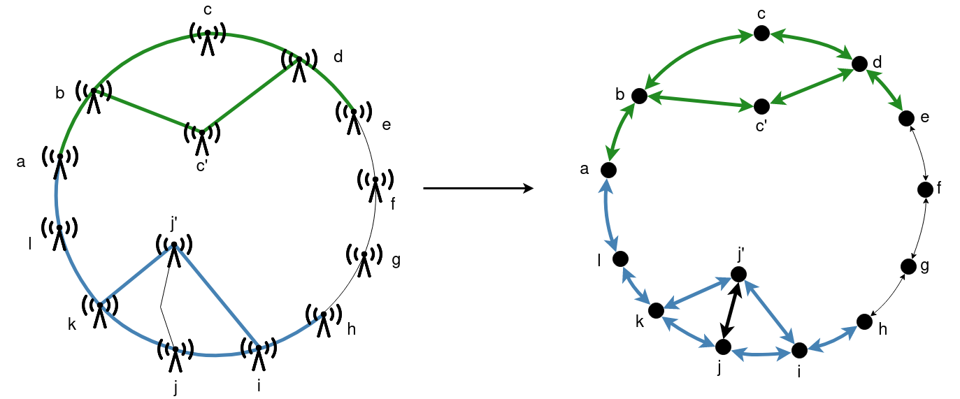
For two nodes of , we say that and are -twins if, starting from a specific time instant , their outside neighbourhoods have a non-empty intersection while the difference between these two sets is less than or equal to a fixed value for consecutive rounds, that is, , for every if and for every otherwise. Fig. 2 exemplifies -twins. We address the following problem.
Periodic-Twins
Input: with representing a time-varying graph of period ; integers and .
Output: for every node in , a list of all its -twins, that is, a list of ’s with being a node ID and the starting time instant where and become -twins for instants.
Note that it is required that the period be given among the input of every node, but not the graph . During each round , every node has a local knowledge of , which is the size of its current neighbourhood, in . In the next Section 3, we prove that Periodic-Twins can be solved after rounds, using messages of size , where is the total number of nodes and is the maximum degree of the graphs ’s.
3 Distributed computation of -twins
The main idea of our solution is based on the following property of static graphs, which hints that every node can compare its -neighbourhood with the -neighbourhood of any other node in its -neighbourhood in order to determine whether that node is one of its -twins. For two nodes of a static graph , we say that and are -twins if they have at least one common neighbour and that the difference between the sets of their outside neighbours is at most , namely . A path of length between and is a path having edges and nodes, of the form with and , for some and .
Property 1
Let be an undirected static graph, let be two distinct nodes in with a common neighbour. Then, and are -twins if and only if or there are at least paths of length between and , where .
Proof
The case when is clear. Otherwise let and . Then, . The paths of length between and are only paths passing through their common neighbours. Therefore, the number of such paths is . We need to prove that and are -twins if and only if . From the definition of -twins, we have . Since , this is equivalent to , in other words, . ∎
Remark 2
Note that and could have very different neighbourhoods. For instance when they have no common neighbours, could be large, while and are not -twins until .
Let be a -periodic time-varying graph with . For every node to compute its list of -twins, we would need rounds per static graph , so that the node collects information about its -neighbourhood. Since the time-varying graph is periodic, we can proceed a first phase of rounds for passing every node’s -neighbourhood information to its neighbours. Then, in a second phase consisting of extra rounds, every node can forward all the pieces of information it has already collected from its neighbours during the first phase. The information received in this second phase informs every node about its -neighbourhood. There are however two drawbacks of the above idea.
Firstly, we need to control the size of the messages sent from each node, especially in the second phase. In Lemma 2 below, we prove that the information related to the entire neighbourhood is not necessary, but only the size of it. Roughly, we plan to only send the size of the neighbourhood each time we need to forward this information. More specifically, following Lemma 2 each node in can determine whether a node in is such that and are -twins at round , by adding the number of ’s neighbours, obtained at round , to the number of ’s neighbours, obtained at round and subtracting the number of common neighbours between them. Then, if the result is less than , they are -twins, according to the inequality given in Lemma 2.
Secondly, we aim at computing -twins in , with representing a continuous window of consecutive time instants starting at . For most this can be done using in the receiver node’s internal storage a counter per sender node, which increments every time the receiver node detects a sender node as its -twin at some . The counter is reset to zero whenever that sender node is detected as a non--twin at some (other) . However, cases involving extremities of interval such as when will have their time window divided into two disjoint intervals: and . If we proceed as with all other cases, the information will be ready at some round after the -th round for this case. We can accelerate this to be as early as in the -th round using internal storage of a table in each receiver node, instead of the previously mentioned incremental counters. Another positive consequence of using a table instead of using incremental counters is that, starting from round , every node has access in real time to its -twins of previous rounds. Then, at the -th round, every node has access to the full list of its -twins, where the computation terminates.
Algorithm 1 implements the above ideas, calling as subroutines both Algorithms 2 and 3 at every round. All tables in Algorithm 1 are dictionary data structures. The result for every node will be stored in table Delta_d_Twins. For its computation, node maintains furthermore two tables, called Twins and Count. For a node with identifier , a strictly positive value of Twins[] means that and have been twin vertices for the last Twins[] number of rounds. Hence, when Twins[] is at least , we append to the resulting list Delta_d_Twins along with the number of rounds where they start to be -twins. This is implemented in Algorithm 3, lines 21-22.
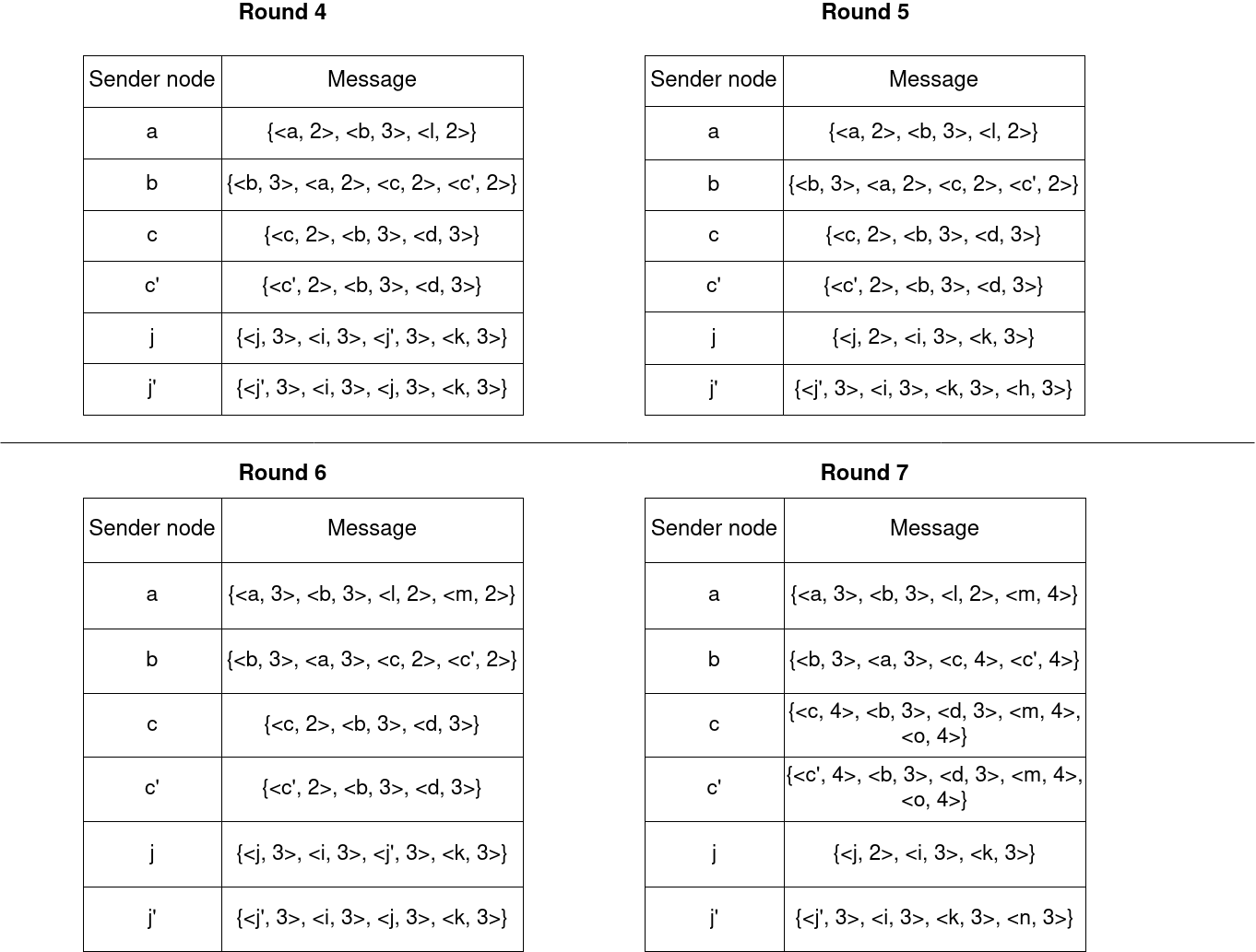
In case we conclude that is not a twin with , such as with Algorithm 3’s lines 12 and 24, a quick way to save this information is to remove key from the (dictionary) table Twins. Table Count is to be used in Algorithm 3 and related to the current round. We use an alternative computation for what is stored in table Count: rather than using Property 1 which would force us to count the number of paths of length , we use the equivalent quantities showed in Lemma 2 below instead. These quantities from Lemma 2 are encoded precisely at line 14 of Algorithm 3. The size of the message in the second phase is composed by two additive terms. The first term is the number of neighbours, multiplied by the size of the nodes ID’s. The second term is the size of the neighbourhood of every neighbour, which is upper bounded by the first term. Thus, the maximum size of messages are bounded by , where is the total number of nodes and is the maximum degree of the graphs ’s, cf. Lemma 1 below. Fig. 3 exemplifies the messages received in the second phase of every node in the example given in Fig. 2.
We now prove the correctness of the algorithm, as well as the maximum size of the messages used in the algorithm.
Lemma 1
Proof
A node can have at most neighbours. For every neighbour of , needs to store the ID of , which requires a size of , and the number of neighbours of , which can be at most , requiring a size . So for a neighbour of , stores information of size , and for all neighbours of , it stores information of size , and this information represents the size of the message that will send in the second phase. ∎
Lemma 2
Given a p-periodic time-varying graph , and two distinct nodes , and are -twins if for that is, for consecutive rounds.
Proof
The proof is very similar to that of Property 1. Let and . From the definition of -twins, we have . Since , this is equivalent to . ∎
The latter lemma allows us to store the -twins in Algorithm 3 and check the number of consecutive round two nodes are -twins in Algorithm 3 line 26 and Algorithm 1 line 20. We have proved the following theorem.
Theorem 3.1
In a -periodic time-varying graph where integers are given as input to every node, problem Periodic-Twins can be solved after rounds, using messages of size , where is the total number of nodes and is the maximum degree of the graphs ’s.
4 Twin sampling with message size
In a static graph, we can reduce the message size as follows. According to Lemma 2 in [6], every node can receive its neighbourhood in a first round, then apply a well selected hash function sampled from a universe of hash functions and forward this to every neighbour in a second round. When receiving the second round message, node can compute the value of within with probability , where and . The process uses messages of size bits. Whence, w.h.p. after rounds the inequality in our Lemma 2 can be decided using messages of bits. For the dynamic case, the extension is similar to construction proposed in Section 3.
5 Conclusion and perspectives
We introduce the problem of finding -twins and propose a distributed algorithm to compute them in any -periodic time-varying graph under a distributed model similar to the -interval-connected network. After rounds, every node can compute the nodes that are its -twins using messages of size , where is the total number of nodes and is the maximum degree of the graphs ’s. Using techniques borrowed from [6], we reduce the message size down to w.h.p. Finding -twins can be useful in several ways. For instance, it could be used for alternately scheduling sleeping times of the twin nodes to save resources, while maintaining connectivity for the rest of the network. Furthermore, it can be used in order to compute disjoint paths or disjoint broadcast trees. As for the next steps of research, it would be useful to extend our algorithm to compute -modules as defined in [5].
References
- [1] Bonnet, E., Kim, E., Thomassé, S., Watrigant, R.: Twin-width I: tractable FO model checking. In: 61st IEEE Annual Symposium on Foundations of Computer Science. pp. 601–612. IEEE (2020)
- [2] Bui-Xuan, B., Hourcade, H., Miachon, C.: Computing temporal twins in time logarithmic in history length. In: 9th International Conference on Complex Networks and their Applications. SCI, vol. 944, pp. 651–663 (2020)
- [3] Casteigts, A., Flocchini, P., Mans, B., Santoro, N.: Measuring temporal lags in delay-tolerant networks. IEEE Trans. Computers 63(2), 397–410 (2014)
- [4] Casteigts, A., Flocchini, P., Quattrociocchi, W., Santoro, N.: Time-varying graphs and dynamic networks. International Journal of Parallel, Emergent and Distributed Systems 27(5), 387–408 (2012)
- [5] Habib, M., Mouatadid, L., Zou, M.: Approximating modular decomposition is hard. In: 6th International Conference on Algorithms and Discrete Applied Mathematics. LNTCS/LNCS, vol. 12016, pp. 53–66 (2020)
- [6] Halldórsson, M., Nolin, A., Tonoyan, T.: Overcoming congestion in distributed coloring. In: 2022 ACM Symposium on Principles of Distributed Computing. pp. 26–36. ACM (2022)
- [7] Kuhn, F., Lynch, N., Oshman, R.: Distributed computation in dynamic networks. In: 42nd ACM Symposium on Theory of Computing. pp. 513–522. ACM (2010)
- [8] Luna, G.D., Viglietta, G.: Computing in anonymous dynamic networks is linear. In: 63rd Annual Symposium on Foundations of Computer Science. pp. 1122–1133. IEEE (2022)
- [9] O’Dell, R., Wattenhofer, R.: Information dissemination in highly dynamic graphs. In: DIALM-POMC Joint Workshop on Foundations of Mobile Computing. pp. 104–110. ACM (2005)