A multi-scale multi-lane model for traffic regulation via autonomous vehicles
Paola Goatin111
Université Côte d’Azur, Inria, CNRS, LJAD, Sophia Antipolis, France. E-mail:
paola.goatin@inria.frBenedetto Piccoli222Rutgers University - Camden, Camden, New Jersey, USA. E-mail:
piccoli@camden.rutgers.edu
Abstract
We propose a new model for multi-lane traffic with moving bottlenecks, e.g., autonomous vehicles (AV). It consists of a system of balance laws for traffic in each lane, coupled in the source terms for lane changing, and fully coupled to ODEs for the AVs’ trajectories.
More precisely, each AV solves a controlled equation depending on the traffic density, while the PDE on the corresponding lane has a flux constraint at the AV’s location. We prove existence of entropy weak solutions, and we characterize the limiting behavior for the source term converging to zero (without AVs), corresponding to a scalar conservation law for the total density.
The convergence in the presence of AVs is more delicate and we show that the limit does not satisfy an entropic equation for the total density as in the original coupled ODE-PDE model. Finally, we illustrate our results via numerical simulations.
Multi-lane traffic has attracted the attention of many researchers in transportation science, in particular applied mathematicians and engineers.
Works on macroscopic models include papers on modeling
[21] and analysis [6, 20].
Recently, extensions to road networks were proposed, see [16, 17].
Starting from these results, we aim at including the presence of autonomous vehicles, which act as moving bottlenecks to regulate traffic, e.g., dissipate traffic waves [1, 35]. Such regulation problems were addressed on a theoretical basis [7, 8, 11, 12, 29, 30, 31, 36, 40, 41], with machine learning approaches [22, 38] and also via real world experiments [18, 34, 39].
A number of approaches were developed to deal with moving bottlenecks [9, 13, 23, 25, 26, 32, 33].
Moreover, extensions to multiple bottlenecks [14] and to second order models [37] were proposed.
In particular we follow the idea of coupling an ODE for the moving bottleneck to a PDE for the bulk traffic as in [9, 10, 13].
The coupling is realized in the ODE right-hand side, which depends on the PDE solution, and by imposing a flux limiter to the PDE at the location of the bottleneck.
Convergence and continuous dependence for such models were achieved [27, 28].
In this work,
we consider a first order macroscopic multi-lane model [6, 20]
of the form
(1.1)
Above, is the number of lanes on the road, is the vehicle density on lane ,
is the flux function
and the average speed is a strictly decreasing function such that and , so that is concave.
The source terms account for
mass exchanges form lane to lane (obviously, ), scaled by a relaxation factor .
Letting , this corresponds to letting to zero the lane-change relaxation parameter.
Throughout the paper, we will assume that
(S0)
, , are Lipschitz continuous in both variables, with Lipschitz constant , and
, and , for all and .
Some results will be subject to further hypotheses:
(S1)
If , then (in particular, by (S0) this implies for all );
(S2)
There exists such that and , for all and .
To account for the presence of an autonomous vehicle (AV) in lane , we model it as a moving bottleneck [9, 13]
reducing to zero the capacity of the lane at the AV position, see also [24]. Let , , be the trajectory of the -th AV travelling on the lane .
The coupling with (1.1) is realized though the following microscopic ODE and constraint:
(1.2a)
(1.2b)
(1.2c)
where is the control law (desired speed) applied to the AV.
Remark that, when the constraint (1.2c) is active, i.e. ,
a non-classical shock arises and
the downstream value of the density must be zero: , while .
In particular, , where is defined by the unique root of the equation .
We refer the reader to Figure 1 for a graphical representation.
(a)AV speed
(b)reduced flow at the AV position
Figure 1: Graphical representation of the AV speed (1.2a) and the corresponding flow constraint (1.2c) introducing the corresponding notation.
We first provide existence results
for the coupled system (1.1)-(1.2),
under assumption (S0),
using the wave-front tracking approximation for a fixed
and assuming bounded variation for the initial datum and the AV control law. Bounds on the total variation are achieved via a careful analysis of the contribution of the source terms and non-classical shocks which may appear at AV locations.
Unfortunately, Lipschitz-type estimates cannot be achieved uniformly in .
Therefore, we first study the limit as without AVs, which is given by the solution of a scalar conservation law for the sum of the densities over all the lanes.
Such convergence is achieved under assumptions (S0) and (S1), adapting a technique originally designed for a chromatography problem, see [4].
We then focus on the case of two lanes and a single AV,
under assumptions (S0), (S1), and (S2).
Even in this simplified setting, we show that in the limit
we do not recover the entropy weak solutions in the sense of [9], attesting the richness of the model.
To further illustrate our results, we provide numerical simulations via finite volume schemes.
We start illustrating the dynamics on a 3-lane road with AVs and different speeds. An oscillatory pattern emerges due to the uneven distribution of traffic among lanes.
We then pass to investigate numerically the convergence as with and without AVs.
In particular, we show the difference between the limit of solutions with AVs and the scalar model proposed in [9]
for the sum of densities.
This paper provide further comprehension of the complexities arising when coupling multi-lane traffic with moving bottlenecks, e.g. AVs. Natural next steps include characterizing futher the limit as , understanding continuous dependence, and extending the theory to networks.
2 Existence of solutions: Wave-front tracking approximations and compactness estimates
The multi-lane model including moving bottlenecks reads:
(2.3)
Solutions to (2.3)
are intended in the following weak sense.
Definition 1.
The -tuple , with
provides a solution
to (2.3) with
if the following conditions hold for , :
1.
and
for all ;
2.
;
3.
For every and for all it holds
(2.4)
4.
For a.e. ,
;
5.
For a.e. , .
Existence and uniqueness without moving bottlenecks have been provided in [16, 20].
To include moving bottlenecks, we can use the techniques developed in [13, 24].
From now on, we consider for simplicity only one AV, say on lane . We denote by its trajectory, and by its desired velocity.
We therefore focus on the well-posedness of the strongly coupled problem
(2.5)
We will prove the following existence result.
Theorem 1.
Under hypotheses (S0), let the initial conditions for , have finite total variation, and also have finite total variation.
Then, for any , there exists a solution of (2.5) in the sense of Definition 1.
For the proof, we proceed similarly to [13, 15].
We approximate the initial data by a sequence of piece-wise constant functions , , such that
each has a finite number of discontinuities and
Analogously, we approximate with piece-wise constant functions with a finite number of discontinuities and such that
Consider a sequence of time steps , ,
such that .
We construct a sequence
of approximate solutions to (1.1)-(1.2) using the Wave Front Tracking (WFT) and operator splitting algorithms as follows.
For any , we set , .
On the time interval , , we define as the WFT approximation of
(2.6)
constructed as described in [3, Chapter 7] or [1, Chapter A.7]. Note that, due to the presence of the source term, we cannot employ a fixed grid as in [3, Chapter 6], see also [13, Section 3.1].
At time , we set
(2.7)
This sequence of approximate solutions satisfies the following compactness estimates.
Lemma 1.
Let (S0) hold and . If for all , then the approximate solutions satisfy
Since the homogeneous step (2.6) does not alter the invariant domain, we focus on (2.7).
We proceed by induction and assume for all .
Denoting , we get by hypotheses
where we have used the Mean Value Theorem setting and for some , , and we have exploited (S) and the hypothesis .
Similarly,
with and for some , with , .
∎
Lemma 2.
Let (S0) hold and , then the approximate solutions satisfy
(2.8)
for , where .
In particular, the sequence total variation in space is uniformly bounded for all .
Proof.
We consider the Glimm type functional
(2.9)
where and is given by
we have that . Of course, for , where the AV is not present, we have
.
It is not restrictive to assume that jump locations in do not coincide for different . Denoting by and respectively the left and right traces of at a jump discontinuity, we get from (2.7)
for some .
By (S), we have that
provided that . Therefore we conclude that
Finally, we get the uniform TV bounds (independent of )
(2.10)
(2.11)
Setting we get the desired estimate.
∎
Lemma 3.
Let (S0) hold and , then for any , , the approximate solutions satisfy
where is independent of (with ) and .
In particular, the Lipschitz constant does not depend on but blows-up as .
Proof.
Let us fix such that
and suppose that there are time steps between and :
Thus,
We observe that, due to finite wave-propagation speed, we have
where is the maximum of the Lipschitz constant of and the maximal AV speed. Moreover, by (2.7),
Let us define
and set
for some .
Using the above notations, we develop
where, by abuse of notation, we set .
Moreover, it holds
where we have set , , with
and for some .
Therefore, we get
which gives the desired -Lipschitz in time estimate uniform in for any fixed.
We observe that the estimate blows-up as , therefore not allowing to pass to the limit directly in (2.5).
∎
Remark 1.
From the above estimates, we note that uniform Lipschitz continuity does not hold even if (i.e. the initial data are at equilibrium).
Proof of Theorem 1.
For any , the previous lemmas provide the compactness estimates on that ensure the existence of a subsequence, still denoted by , converging in to some function such that
for a.e. (Helly’s Theorem), so that point 1
in Definition 1 is satisfied.
Concerning , by construction we have that for a.e. and . Hence, by the Ascoli-Arzela Theorem, there exists a subsequence, still denoted by converging uniformly to a function , which is also Lipschitz of constant .
Following [13, Proof of Lemma 3.4], one can prove also that has uniformly bounded total variation on .
Here, in addition to jumps due to interactions with waves coming from the right and jumps in the control function , we have jumps induced by the relaxation step (2.7) at any . In this case, can be increasing only if decreases at .
This increment is bounded by
, thus
in total
(note that this bound is not uniform in ).
Therefore, converges to in and , see Definition 1, point 2.
Proceeding as in [13, Proof of Theorem 3.1], we get that the satisfies
points 3 and 4
in Definition 1.
We are now left with Definition 1, point 5. To this end, we follow [28, Section 3.3] and [13, Section 3],
but note that, in our case, , where is implicitly defined by , and we have the additional source term in (2.7).
Fix and, possibly discarding a set of zero measure, without loss
of generality assume:
1.
, ;
2.
continuously differentiable at and ;
3.
;
4.
for a.e. , and for every , .
From 4. we have that step (2.7) does not occur at for any , thus is constructed only by wave-front tracking on a sufficiently small open interval containing . Therefore, we can follow the same strategy of [28, Section 3.3] and [13, Section 3].
By 2. and 3., point 5 of Definition 1 is satisfied if
(2.12)
Since by 1. ,
(2.12) holds true if
and
for infinitely many .
From 4., if
for sufficiently large, then we also have
.
Define , then we can restrict to the case , which implies .
We distinguish two cases:
1.
:
First, notice that Lemma 1 and Lemma 4 of [28] hold true since they are based only on TV bounds that still hold. For some sufficiently small,
we have that .
Then the proof of Lemma 6 of [28] still holds,
since it is based on Lemma 4 and the fact that . We conclude in the same way as in
[28, Section 3.3.1].
2.
: In this case, we have .
Following [28, Section 3.3.1], if
for an infinite number of indices , then we conclude by Lemma 4 that (2.12) holds true.
Assume now that
for sufficiently big. Fix , then
again by Lemma 4 of [28], there exists such that the following holds true. The function takes values in on the interval , and takes values in on the interval
.
Since is generated by wave-front tracking,
on the interval it may contain only shocks, non-classical shocks, and rarefaction shocks.
The only admissible non-classical shock is .
If contains a non-classical shock for infinitely many , then the non-classical shock must be located at and by 3. .
Now, by Lemma 1 of [28], for large enough, any rarefaction shock contained in has strength less than , thus we deduce that takes values in on the interval , except possibly to the right of the non-classical shock located at .
In this case, a classical big shock
is present to the right of connecting to a value .
This big shock is followed by small waves, classical shocks or rarefaction shocks, with left and right-hand states in
.
Since these small waves have speed strictly lower than the non-classical shock and the big classical shock, they interact with both of them within time
time ,
where is the speed of the non-classical shock and
is the maximum
speed of the small waves, thus
.
In particular,
we can follow the proof
of Lemmas 13 and 14 of [28],
thus also Lemma 10 of [28] holds true.
Since is arbitrarily small, we can conclude as in [28, Section 3.3.3].
In this section we assume that no AV is present, thus we focus on the multi-lane model [20]:
(3.13)
In this case, the definition of entropy weak solution reduces to:
Definition 2.
A function is a entropy weak solution of (3.13) with if
for every and for all it holds
(3.14)
for .
We extend the stability result given in [20, Theorem 3.3] taking in account flux dependency.
Besides (3.13), we consider
(3.15)
with satisfying the same hypotheses as (, Lipschitz and concave).
Lemma 4.
Under hypothesis (S0), let and be respectively the entropy weak solutions of (3.13) and (3.15), and
let , . Then, for a.e. it holds
(3.16)
In particular, the above estimate is independent of .
Proof.
Let us consider WFT approximate solutions constructed by fractional steps as in Section 2.
Given a sequence of time steps , ,
such that , let and the sequences of WFT approximations to (3.13) and (3.15) such that,
setting , for any fixed:
•
In any time interval , , is the WFT approximation of
(3.17)
and is the WFT approximation of
(3.18)
constructed as described e.g. in [19, Section 2.3].
see e.g. [2, Section 3].
Indeed, by [20, Corollary 3.4], we know that for all
Subtracting (3.20) from (3.19) and setting
and for , we get (using notations introduced earlier for the partial derivatives of the terms )
Since and by hypothesis and for sufficiently small, we conclude that if
for all , then
for all .
Then, by the Crandall-Tartar lemma [19, Lemma 2.13], we get
(3.22)
Putting together (3.21) and (3.22), we obtain the desired estimate.
∎
Let us now assume:
(V)
(in particular, the maximal speeds become ) and the maximal density on each lane (so that ),
and thus , for all .
Lemma 5.
Under hypotheses (S0), (S1) and (V), let the initial data for , be at equilibrium, i.e.
(3.23)
Then the solution stays at equilibrium, i.e.
for all , . In particular, the solution is -Lipschitz continuous in time, uniformly in :
(3.24)
for any , with .
The proof is trivial observing that system (3.13) reduces to identical equations with the same initial datum, and therefore for all .
The uniform Lipschitz estimate (3.24) and the uniform TV bound (2.8) allow to apply Helly’s Theorem to the sequence , proving the existence of a subsequence converging in (indeed, the sequence is constant for all , so there is nothing to prove). In particular, the limit satisfies for any and it holds
so that, setting , is a entropy weak solution to the scalar Cauchy problem
(3.25)
where we have set .
We can now give the following result about the convergence of (3.13) to (3.25) as .
Theorem 2.
Under hypotheses (S0), (S1) and (V), let and be the corresponding solution of (3.13).
Then, for each ,
as , where is the entropy weak solution of (3.25).
Proof.
We adapt an argument by Bressan and Shen [4, Section 5].
Denote by the solution of
(3.26)
with the same initial data . Linearizing (3.26) around the equilibrium initial condition with for we obtain
where we have set and
is a tridiagonal matrix such that
The similarity transformation to a symmetric matrix
gives
which, by the monotonicity hypotheses in , turns out to be negative definite (this can be easily seen applying Sylvester’s criterion).
Therefore,
(3.27)
Moreover, for any interval , comparison between (3.13) and (3.26) gives, by Lemma 4,
Let (S0) and (S2) hold and , then for any , , the approximate solutions satisfy
(4.30)
where is independent of and
Proof.
We follow the same procedure and notations as in the proof of Lemma 3.
Setting
we compute
Moreover, for , it holds
where we have set , , with
and for some .
Therefore, we get
where we have used the inequality
, which holds provided
that .
∎
Remark 2.
By Lemma 6, the Lipschitz constant is uniformly bounded as for any strictly positive time. Indeed, taking with in (4.30), we have
(4.31)
which goes to zero with .
Note also that, under the hypotheses of Lemma 6, if the initial datum is at equilibrium, i.e. for a.e. , it holds for all . Therefore, the approximate solutions are uniformly Lipschitz continuous for all :
(4.32)
We can now prove the following convergence result.
Theorem 3.
Under hypotheses (S0), (S1) and (S2), let
(thus )
and
and and be the corresponding entropy weak solution of (4.29).
Then
as , where and
is a weak solution of (3.25) with .
If moreover in
, then
satisfies
(4.33)
with .
Remark 3.
We notice that, as pointed out in the proof of Theorem 1, we need to assume a-priori the convergence of the AV trajectories to .
Theorem 3 shows in particular that cannot be an entropy weak solution of the moving bottleneck model [9, 13] with , which writes
(4.34)
where , whose entropy weak solution satisfies
(4.35)
Observe that we can estimate
taking . This shows that (4.35) implies (4.33), but the converse is not true. See also the numerical examples in Section 5.3.
Proof of Theorem 3.
By Helly’s Theorem, for any there exists a subsequence such that converges to some function in .
We can then construct by diagonal process a sequence, still labeled , converging to in . From (4.30) and (4.31), the limit satisfies
for all .
Passing to the limit as and summing over , we get
concluding the proof.
5 Numerical simulations
To illustrate the behaviour of solutions of model (2.3), we compute approximate solutions obtained via a finite volume scheme with time splitting developed merging the numerical schemes proposed in [16] for multi-lane models and in [5] for correctly capturing the dynamics around moving bottlenecks. See also [14, 17, 37] for further extensions.
We consider a uniform space mesh of width and a time step , subject to the stability condition
see Lemma 1.
We set
and
for ,
where is the center of cell and are the
interfaces. Set .
We approximate the initial data as
The approximate solutions to (1.1) are obtained through a Godunov type scheme with fractional step accounting for the contribution of the source term: for , and , we set
(5.39)
where
with
being the point of maximum of .
To capture the presence of an AV, let’s say at position in lane , we modify the Godunov fluxes at the interfaces as follows.
We denote by the standard Riemann solver for
,
i.e. gives the value of the self-similar entropy weak solution corresponding to the Riemann initial data at .
We also set
the discretization of the AV’s desired speed.
If
(5.40)
we expect the flux constraint to be active at
with
to ensure mass conservation. If , then and, setting , we replace the numerical fluxes in (5.39) by
Besides, to track the AV’s trajectory, at each time step we implement an explicit Euler scheme:
In the following numerical tests we consider (2.3) with
(5.41a)
(5.41b)
(5.41c)
5.1 A 3-lane road with heterogeneous speed limits and AVs
As an illustration of the behaviour of model (2.3), we consider and for .
We set for and km/h, km/h, km/h, thus considering different speed limits on each lane. AVs’ desired speeds are set constantly to km/h and the relaxation parameter .
We consider a road stretch of length km with and initial conditions
(5.42)
for the (normalized) traffic densities on each lane, and
for the AVs’ positions.
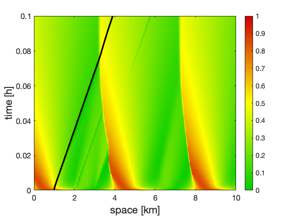
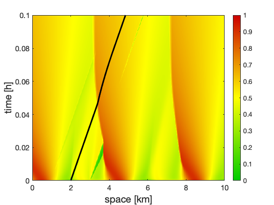
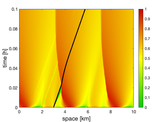
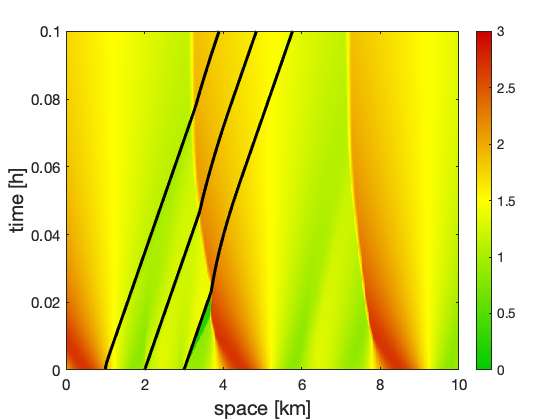
(a)Density and trajectory on lane 1
(b)Density and trajectory on lane 2
(c)Density and trajectory on lane 3
(d)Total density and AVs’ trajectories
Figure 2: Heat-map of the traffic densities on each lane and the total density on the road segment km and the time interval h, with the corresponding AV’s trajectories (black lines).
In Figure 2, we can observe that, due to the different speed limits, vehicles tend to move and accumulate into the fastest lanes 2 and 3, while lane 1 remains almost empty. Also, due to low traffic, on lane 1 there is no interaction between the AV and the bulk traffic. On the contrary, in Figure 2(c) we can observe the appearance of non-classical shocks. Moreover, we may observe that AVs slow down to adapt to the downstream traffic speed both in Figures 2(b) and 2(c). Figure 2(d) gives an overview of the total traffic density on the three lanes, showing that an oscillatory pattern in the density can still be observed due to the uneven distribution of the traffic density across lanes.
5.2 Relaxation limit without AVs
To illustrate the convergence result proved in Section 3 (see Theorem 2), we consider the same scenario as in the previous Section 5.1, i.e. , for and initial density data as in (5.42). Now, no AVs are present.
We consider two cases:
(C1)
km/h, so that the speed function is the same on all lanes and we fulfill the hypotheses of Theorem 2;
(C2)
km/h, km/h, km/h, to be compared with the solution of the conjectured limit LWR equation (3.25) with speed flux function , , where km/h is the average maximal speed among lanes 1 to 3. Note that this is indeed the relaxation limit in case (C1).
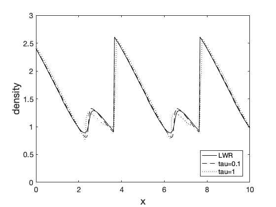
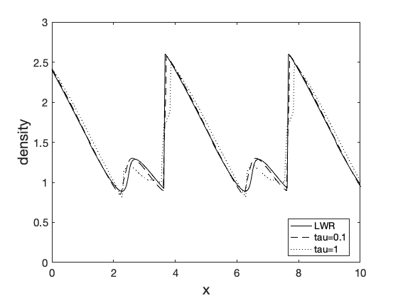
(a) km/h
(b), , km/h
Figure 3: Density profiles at min of the total densities of model (3.13) with and the solution of LWR model (3.25) for cases (C1) (left) and (C2) (right).
Figure 3 shows the profiles of the total density for model (3.13) for and and the solution of the limit LWR problem (3.25) at time min. In particular, in Figure 3(a) we can observe an illustration of relaxation limit stated in Theorem 2. Moreover, Figure 3(b) suggests that the limit also holds for non homogeneous speeds on the different lanes, as conjectured in the design of test (C2).
5.3 Relaxation limit with AV
Referring to the results in Section 4, we aim at comparing the relaxation limit of model (4.29), i.e. the multi-lane model with lanes and a single AV, with the solution of the corresponding moving bottleneck model (4.34).
We take , (thus ),
so that and .
Moreover, we set .
We consider different density initial data and AV speeds, to see when non-classical shocks appear in the solution of (4.29) and to understand their nature. In the following, we denote by and respectively the left and right traces of the non-classical shock in (4.34),
the density
satisfying and the density
satisfying .
Setting , we get , and . Accordingly, we consider the following constant initial data:
(IC1)
, i.e. ;
(IC2)
, i.e. ;
(IC3)
, i.e. ;
(IC4)
, i.e. ;
(IC5)
, i.e. .
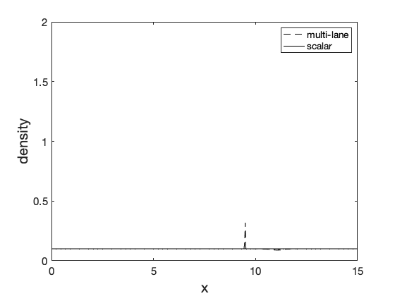
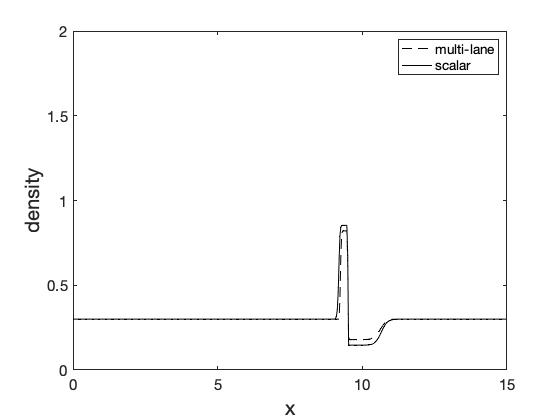
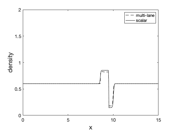
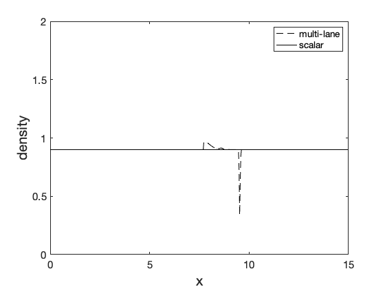
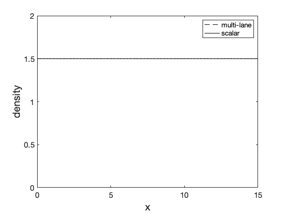
The corresponding density profiles at are displayed in Figure 6. It appears clearly that, when the AV acts as a flux constraint, the density traces at the AV location differ between model (4.29) and (4.34). In particular, we observe that we always have .
(a)(IC1)
(b)(IC2)
(a)(IC3)
(b)(IC4)
(a)(IC5)Figure 6: Comparison between solutions of (4.29) with and solution of (4.34),
with , for .
Appendix A stability for systems of weakly coupled balance laws
Let us consider the systems of balance laws coupled in the source term
Note that, setting in (A.44), one recovers the classical stability estimate for scalar equations. Instead, (3.16) is stronger than (A.44), due to the specific monotonocity assumption (S0). In particular, estimate (A.44) does not suffice to conclude in the proof of Theorem 2, since in this case and we get
[2]
S. Bianchini.
The semigroup generated by a Temple class system with non-convex
flux function.
Differential Integral Equations, 13(10-12):1529–1550, 2000.
[3]
A. Bressan.
Hyperbolic systems of conservation laws, volume 20 of Oxford Lecture Series in Mathematics and its Applications.
Oxford University Press, Oxford, 2000.
The one-dimensional Cauchy problem.
[4]
A. Bressan and W. Shen.
BV estimates for multicomponent chromatography with relaxation.
Discrete Contin. Dynam. Systems, 6(1):21–38, 2000.
[5]
C. Chalons, M. L. Delle Monache, and P. Goatin.
A conservative scheme for non-classical solutions to a strongly
coupled PDE-ODE problem.
Interfaces Free Bound., 19(4):553–570, 2017.
[6]
R. M. Colombo and A. Corli.
Well posedness for multilane traffic models.
Ann. Univ. Ferrara Sez. VII Sci. Mat., 52(2):291–301, 2006.
[7]
C. Daini, M. L. Delle Monache, P. Goatin, and A. Ferrara.
Traffic Control via Fleets of Connected and Automated Vehicles.
working paper or preprint, 2023.
[8]
C. Daini, P. Goatin, M. L. D. Monache, and A. Ferrara.
Centralized traffic control via small fleets of connected and
automated vehicles.
In 2022 European Control Conference (ECC), pages 371–376,
2022.
[9]
M. L. Delle Monache and P. Goatin.
Scalar conservation laws with moving constraints arising in traffic
flow modeling: an existence result.
J. Differential Equations, 257(11):4015–4029, 2014.
[10]
M. L. Delle Monache and P. Goatin.
Stability estimates for scalar conservation laws with moving flux
constraints.
Netw. Heterog. Media, 12(2):245–258, 2017.
[11]
M. L. Delle Monache, T. Liard, A. Rat, R. Stern, R. Bhadani, B. Seibold,
J. Sprinkle, D. B. Work, and B. Piccoli.
Feedback Control Algorithms for the Dissipation of Traffic Waves
with Autonomous Vehicles, pages 275–299.
Springer International Publishing, Cham, 2019.
[12]
A. Ferrara, G. P. Incremona, E. Birliba, and P. Goatin.
Multi-scale model based hierarchical control of freeway traffic via
platoons of connected and automated vehicles.
IEEE Open Journal of Intelligent Transportation Systems, pages
1–1, 2022.
[13]
M. Garavello, P. Goatin, T. Liard, and B. Piccoli.
A multiscale model for traffic regulation via autonomous vehicles.
J. Differential Equations, 269(7):6088–6124, 2020.
[14]
P. Goatin, C. Daini, M. L. Delle Monache, and A. Ferrara.
Interacting moving bottlenecks in traffic flow.
Netw. Heterog. Media, 18(2):930–945, 2023.
[15]
P. Goatin and N. Laurent-Brouty.
The zero relaxation limit for the Aw-Rascle-Zhang traffic flow
model.
Z. Angew. Math. Phys., 70(1):Paper No. 31, 24, 2019.
[16]
P. Goatin and E. Rossi.
A multilane macroscopic traffic flow model for simple networks.
SIAM J. Appl. Math., 79(5):1967–1989, 2019.
[17]
P. Goatin and E. Rossi.
Comparative study of macroscopic traffic flow models at road
junctions.
Netw. Heterog. Media, 15(2):261–279, 2020.
[18]
G. Gunter, D. Gloudemans, R. E. Stern, S. McQuade, R. Bhadani, M. Bunting,
M. L. Delle Monache, R. Lysecky, B. Seibold, J. Sprinkle, et al.
Are commercially implemented adaptive cruise control systems string
stable?
IEEE Transactions on Intelligent Transportation Systems,
22(11):6992–7003, 2020.
[19]
H. Holden and N. H. Risebro.
Front tracking for hyperbolic conservation laws, volume 152 of
Applied Mathematical Sciences.
Springer, Heidelberg, second edition, 2015.
[20]
H. Holden and N. H. Risebro.
Models for dense multilane vehicular traffic.
SIAM J. Math. Anal., 51(5):3694–3713, 2019.
[21]
A. Klar and R. Wegener.
A hierarchy of models for multilane vehicular traffic. I.
Modeling.
SIAM J. Appl. Math., 59(3):983–1001, 1999.
[22]
A. R. Kreidieh, C. Wu, and A. M. Bayen.
Dissipating stop-and-go waves in closed and open networks via deep
reinforcement learning.
In 2018 21st International Conference on Intelligent
Transportation Systems (ITSC), pages 1475–1480, 2018.
[23]
C. Lattanzio, A. Maurizi, and B. Piccoli.
Moving bottlenecks in car traffic flow: a PDE-ODE coupled model.
SIAM J. Math. Anal., 43(1):50–67, 2011.
[24]
N. Laurent-Brouty, G. Costeseque, and P. Goatin.
A macroscopic traffic flow model accounting for bounded
acceleration.
working paper or preprint, Feb. 2020.
[25]
J. Lebacque, J. Lesort, and F. Giorgi.
Introducing buses into first-order macroscopic traffic flow models.
Transportation Research Record, 1644(1):70–79, 1998.
[26]
L. Leclercq, S. Chanut, and J.-B. Lesort.
Moving bottlenecks in Lighthill-Whitham-Richards model: A unified
theory.
Transportation Research Record, 1883(1):3–13, 2004.
[27]
T. Liard and B. Piccoli.
Well-posedness for scalar conservation laws with moving flux
constraints.
SIAM Journal on Applied Mathematics, 79(2):641–667, 2019.
[28]
T. Liard and B. Piccoli.
On entropic solutions to conservation laws coupled with moving
bottlenecks.
Commun. Math. Sci., 19(4):919–945, 2021.
[29]
T. Liard, R. E. Stern, and M. L. Delle Monache.
A PDE-ODE model for traffic control with autonomous vehicles.
Networks and Heterogenous Media, 5 2022.
[30]
G. Piacentini, P. Goatin, and A. Ferrara.
Traffic control via moving bottleneck of coordinated vehicles.
IFAC-PapersOnLine, 51(9):13–18, 2018.
[31]
G. Piacentini, P. Goatin, and A. Ferrara.
Traffic control via platoons of intelligent vehicles for saving fuel
consumption in freeway systems.
IEEE Control Syst. Lett., 5(2):593–598, 2021.
[32]
R. A. Ramadan and B. Seibold.
Traffic flow control and fuel consumption reduction via moving
bottlenecks.
Preprint, https://arxiv.org/pdf/1702.07995.pdf, 2017.
[33]
M. D. Simoni and C. G. Claudel.
A fast simulation algorithm for multiple moving bottlenecks and
applications in urban freight traffic management.
Transportation Research Part B: Methodological, 104:238–255,
2017.
[34]
R. E. Stern, Y. Chen, M. Churchill, F. Wu, M. L. Delle Monache, B. Piccoli,
B. Seibold, J. Sprinkle, and D. B. Work.
Quantifying air quality benefits resulting from few autonomous
vehicles stabilizing traffic.
Transportation Research Part D: Transport and Environment,
67:351–365, 2019.
[35]
R. E. Stern, S. Cui, M. L. D. Monache, R. Bhadani, M. Bunting, M. Churchill,
N. Hamilton, R. Haulcy, H. Pohlmann, F. Wu, B. Piccoli, B. Seibold,
J. Sprinkle, and D. B. Work.
Dissipation of stop-and-go waves via control of autonomous vehicles:
Field experiments.
Transportation Research Part C: Emerging Technologies,
89:205–221, 2018.
[36]
A. Talebpour and H. S. Mahmassani.
Influence of connected and autonomous vehicles on traffic flow
stability and throughput.
Transportation Research Part C: Emerging Technologies,
71:143–163, 2016.
[37]
S. Villa, P. Goatin, and C. Chalons.
Moving bottlenecks for the Aw-Rascle-Zhang traffic flow model.
Discrete Contin. Dyn. Syst. Ser. B, 22(10):3921–3952, 2017.
[38]
E. Vinitsky, K. Parvate, A. Kreidieh, C. Wu, and A. Bayen.
Lagrangian control through deep-rl: Applications to bottleneck
decongestion.
In 2018 21st International Conference on Intelligent
Transportation Systems (ITSC), pages 759–765, 2018.
[39]
F. Wu, R. E. Stern, S. Cui, M. L. Delle Monache, R. Bhadani, M. Bunting,
M. Churchill, N. Hamilton, B. Piccoli, B. Seibold, et al.
Tracking vehicle trajectories and fuel rates in phantom traffic jams:
Methodology and data.
Transportation Research Part C: Emerging Technologies,
99:82–109, 2019.
[40]
M. Čičić and K. H. Johansson.
Traffic regulation via individually controlled automated vehicles: a
cell transmission model approach.
In 2018 21st International Conference on Intelligent
Transportation Systems (ITSC), pages 766–771, 2018.
[41]
M. Čičić and K. H. Johansson.
Stop-and-go wave dissipation using accumulated controlled moving
bottlenecks in multi-class CTM framework.
In 2019 IEEE 58th Conference on Decision and Control (CDC),
pages 3146–3151, 2019.