figurec
PHYSTAT Informal Review:
Marginalizing versus Profiling of Nuisance Parameters
Notes by
Robert D. Cousins
Department of Physics and Astronomy
University of California, Los Angeles 90095
Los Angeles, CA
and
Larry Wasserman
Department of Statistics and Data Science
Carnegie Mellon University
Pittsburgh, PA 15213
Abstract
This is a writeup, with some elaboration, of the talks by the two authors (a physicist and a statistician) at the first PHYSTAT Informal review on January 24, 2024. We discuss Bayesian and frequentist approaches to dealing with nuisance parameters, in particular, integrated versus profiled likelihood methods. In regular models, with finitely many parameters and large sample sizes, the two approaches are asymptotically equivalent. But, outside this setting, the two methods can lead to different tests and confidence intervals. Assessing which approach is better generally requires comparing the power of the tests or the length of the confidence intervals. This analysis has to be conducted on a case-by-case basis. In the extreme case where the number of nuisance parameters is very large, possibly infinite, neither approach may be useful. Part I provides an informal history of usage in high energy particle physics, including a simple illustrative example. Part II includes an overview of some more recently developed methods in the statistics literature, including methods applicable when the use of the likelihood function is problematic.
Foreword
This document collects reviews written by Bob Cousins, Distinguished Professor Emeritus in the Department of Physics and Astronomy at UCLA, and Larry Wasserman, Professor of Statistics and Data Science at Carnegie Mellon University, on inferential methods for handling nuisance parameters.
These notes expand upon the main points of discussion that arose during the first of a new event series called PHYSTAT–Informal Reviews, which aims to promote dialogue between physicists and statisticians on specific topics. The inaugural event held virtually on January 24, 2024, focused on the topic of "Hybrid Frequentist and Bayesian approaches". Bob Cousins and Larry Wasserman presented excellent talks, and the meeting was further enriched by a valuable discussion involving the statisticians and physicists in the audience.
In Part I, Bob Cousins provides a comprehensive overview of how high-energy physicists have historically tackled the problem of inferring a parameter of interest in the presence of nuisance parameters. The note offers insights into why methods like profile likelihood are somewhat dominant in practice while others have not been widely adopted. Various statistical solutions are also compared through a classical example with relevance in both physics and astronomy. This memorandum is a wealth of crucial references concerning statistical practice in the physical sciences.
In Part II, Larry Wasserman examines the problem of conducting statistical inference with nuisance parameters from the perspectives of both classical and modern statistics. He notes that standard inferential solutions require a likelihood function, regularity conditions, and large samples. Nonetheless, recent statistical developments may be used to ensure correct coverage while relaxing these requirements. This review offers an accessible self-contained overview of some of these approaches and guides the reader through their strengths and limitations.
Together, the written accounts below provide a cohesive review of the tools currently adopted in the practice of statistical inference in searches for new physics, as well as their historical and technical justification. They also offer a point of reflection on the role that more sophisticated statistical methods and recent discoveries could play in assisting the physics community in tackling both classical and new statistical challenges.
The organizing committee of PHYSTAT activities is grateful to both authors for their engagement and valuable contributions, which we believe will benefit both the statistics and physics communities.
Sara Algeri,
School of Statistics, University of Minnesota, Minneapolis, MN
On behalf of the PHYSTAT Organizing Committee
Part I: Physicist’s View
by Robert D. Cousins
1 Introduction
This is a writeup (with some changes) of the 20-minute talk that I gave at a virtual PhyStat meeting that featured “mini-reviews” of the topic by a physicist (cousinsphystat2023) and a statistician (wassermanphystat2023) Mine was largely based on my talk the previous year at a BIRS workshop at Banff (cousinsbanff2023). This is a short personal perspective through the lens of sometimes-hazy recollections of developments during the last 40 years in high energy physics, and is not meant to be a definitive history. I also refer at times to my lecture notes from the 2018 Hadron Collider Physics Summer School at Fermilab (cousinshcpss2018), which provide a more detailed introduction to some of the fundamentals, such as the duality of frequentist hypothesis testing and confidence intervals (“inverting a test" to obtain intervals).
Parametric statistical inference requires a statistical model, , which gives the probability (density) for observing data , given parameter(s) . In a given context, is partitioned as , where is the parameter of interest (taken to be a scalar in this note, e.g., the magnitude of a putative signal), and is typically a vector of “nuisance parameters” with values constrained by subsidiary measurements, usually referred to as “systematic uncertainties” in particle physics (e.g., detector calibration “constants”, magnitudes of background processes, etc.).
This note discusses the common case in which one desires an algorithm for obtaining “frequentist confidence intervals (CI)” for that are valid at a specified confidence level (CL), no matter what are the unknown values of . Ideally, CIs have exact “frequentist coverage” of the unknown true value of , namely that in imagined repeated applications of the algorithm for different data sampled from the model, in the long run a fraction CL of the confidence intervals will contain (cover) the unknown true . In practice, this is often only approximately true, and some over-coverage (fraction higher than CL) is typically tolerated (with attendant loss of power), while material under-coverage is considered disqualifying.
The construction of confidence intervals requires that for every possible true , one chooses an ordering of the sample space . This is done by specifying an ordered “test statistic”, a function of the observed data and parameters. In the absence of nuisance parameters, standard choices have existed since the 1930s. Thus, a key question to be discussed is how to treat (“eliminate") the nuisance parameters in the test statistic, so that the problem is reduced to the case without nuisance parameters.
A second question to be discussed is how to obtain the sampling distribution of the test statistic under the statistical model(s) being considered. There is a vast literature on approximate analytic methods that become more accurate as the sample size increases. For small sample sizes in particle physics, Monte Carlo simulation is typically used to obtain these distributions. The crucial question is then, which values(s) of the nuisance parameters should be used in the simulations, so that the inferred confidence intervals for the parameter of interest have valid coverage, no matter what are the true values of the nuisance parameters.
Section 2 defines the profile and marginalized likelihoods. Section 3 introduces the two corresponding ways to treat nuisance parameters in simulation, the parametric bootstrap and marginalization (sampling from the posterior distribution of the nuisance parameters). Section 4 is a longer section going into detail regarding five ways to calculate the significance in the on/off problem (ratio of Poisson means). Section 5 briefly highlights the talk by Anthony Davison on this subject at the recent 2023 BIRS workshop at Banff. Section 6 contains some final remarks.
2 Choice of test statistic
The observed data are plugged into the statistical model to obtain the likelihood function . The global maximum is at . The “profile likelihood function" (of only ) is
| (1) |
where, for a given , the restricted estimate maximizes for that . It is also written as
| (2) |
(The restricted estimate is denoted by in reidslac2003.) It is common in HEP to use as a test statistic the “profile likelihood ratio” (PLR) with the likelihood at the global maximum in the denominator,
| (3) |
The “integrated” (or “marginalized”) likelihood function (also of only ) is
| (4) |
where is a weight function in the spirit of a Bayesian prior pdf. (More generally, it could be .)
One can then use either of these as if it were a 1D likelihood function with the nuisance parameters “eliminated”. The question remains, what are the frequentist properties of intervals constructed for ? The long tradition in particle physics is to use the profile likelihood function and the asymptotic theorem of wilks to obtain approximate 1D confidence intervals (as well as multi-dimensional confidence regions in cases beyond the scope of this note). For a brief review, see Section 40.3.2.1 and Table 40.2 of the pdg2022. For decades, a commonly used software tool has been the classic program (originally in FORTRAN and later in C and C++), “Minuit: A System for Function Minimization and Analysis of the Parameter Errors and Correlations” (minuit). MINUIT refers to the uncertainties from profile likelihood ratios as “MINOS errors”, which are discussed by minoscpc. I believe that the name “profile likelihood” entered the HEP mainstream in 2000, thanks to a talk by statistician Wolfgang Rolke on work with Angel López at the second meeting of what became the PhyStat series (rolkeclk; rolkelopez2001; Rolke2005). Interestingly, minoscpc and rolkeclk conceptualize the same math in two different ways, as discussed in my lectures (cousinshcpss2018); this may have delayed recognizing the connection (which was not immediate, even after Wolfgang’s talk).
At some point, a few people started integrating out nuisance parameter(s), typically when there was a Gaussian/normal contribution to the likelihood, while treating the parameter of interest in a frequentist manner. One of the earlier examples (citing yet earlier examples) was by myself and Virgil Highland, “Incorporating systematic uncertainties into an upper limit” (cousinshighland). We looked at the case of a physics quantity (cross section) , where is an unknown Poisson mean and is a factor called the integrated luminosity. One observes a sampled value from the Poisson distribution. From , one can obtain a usual frequentist upper confidence limit on . If is known exactly, one then simply scales this by to get an upper confidence limit on . We considered the case in which, instead, one has an independent unbiased measurement of with some uncertainty, yielding a likelihood function of . Multiplying by a prior pdf for yields a Bayesian posterior pdf for . We advocated using this as a weight function for what we now call integrating/marginalizing over the nuisance parameter . A power series expansion gave useful approximations.
Our motivation was to ameliorate an effect whereby confidence intervals derived from a discrete observable become shorter when a continuous nuisance parameter is added to the model. In the initially submitted draft, we did not understand that we were effectively grafting a Bayesian pdf onto a frequentist Poisson upper limit. Fred James sorted us out before publication. A more enlightened discussion is in my paper with Jim Linnemann and Jordan Tucker (CLT), referred to as CLT, discussed below. Luc Demortier noted that, in these simple cases, what we did was the same math as Bayesian statistician George Box’s prior predictive -value (box1980; CLT). Box calculated a tail probability after obtaining a Bayesian pdf, and we averaged a frequentist tail probability over a Bayesian pdf. The two calculations simply reverse the order of two integrals.
A key paper was submitted in the first year of LHC data taking, by Glen Cowan, Kyle Cranmer, Eilam Gross, and Ofer Vitells (CCGV), “Asymptotic formulae for likelihood-based tests of new physics” (ccgv2011). They provided useful asymptotic formulas for the PLR and their preferred variants, which have been widely used at the LHC and beyond. I believe that this had a significant side effect: since asymptotic distributions were not known in HEP for other test statistics, the default became PLR variants in CCGV, even for small sample size, in order to have consistency between small and large sample sizes.
Meanwhile, in the statistics literature, there is a long history of criticism of the simple PLR. At PhyStat meetings, various higher-order approximations have been discussed by Nancy Reid at SLAC in reidslac2003; by Nancy (reidoxford2005; reidoxford2) and me (cousinsoxford2005) at Oxford in 2005; by Anthony Davidson in the Banff Challenge of 2006 (davisonbanffchallenge), at PhyStat-nu 2019 (davison2019), and at Banff last year davisonbanff2023; and by statistician Alessandra Brazzale (brazzalephystat2019) and physicist Igor Volobouev and statistician Alex Trindale at PhyStat-DM in volobouevphystat2019. Virtually none of these developments have been adopted for widespread use in HEP, as far as I know.
Bayesian statisticians at PhyStat meetings have long advocated marginalizing nuisance parameters, even if we stick to frequentist treatment of the parameter of interest, e.g., James Berger, Brunero Liseo, and Robert Wolpert, “Integrated Likelihood Methods for Eliminating Nuisance Parameters”, (berger1999). Berger et al., in their rejoinder to a comment by Edward Susko, wrote, “Dr. Susko finishes by suggesting that it might be useful to compute both profile and integrated likelihood answers in application, as a type of sensitivity study. It is probably the case that, if the two answers agree, then one can feel relatively assured in the validity of the answer. It is less clear what to think in the case of disagreement, however. If the answers are relatively precise and quite different, we would simply suspect that it is a situation with a ‘bad’ profile likelihood.” I agree with Susko’s suggestion to compute (and report) both profile and integrated likelihood answers, to build up experience and to see if Berger et al. are right in real cases relevant to HEP.
However, in my experience, marginalizing nuisance parameters is relatively rare at the LHC. This is for various reasons, in my opinion, including:
-
•
The historical traditions of frequentist statistics in HEP, and the naturalness of PLRs as test statistics;
-
•
In particular, the historical precedent of MINUIT MINOS;
-
•
The (false) impression that doing something Bayesian-inspired is unjustifiable to a frequentist, when frequentist calibration measures can provide the justification.
-
•
The asymptotic formulas of CCGV are readily available for profile likelihood but not for marginalization, and are the default in the now-dominant software tools.
It also seems common that the minimization required for profiling is less CPU-intensive than the integration required for marginalization.
Thus, the profile likelihood ratio (including variants with parameters near boundaries as in CCGV (ccgv2011)) is the most common test statistic in use today at the LHC, and perhaps in all of HEP. Among other uses, it is the basis of the ordering for confidence intervals advocated by Gary Feldman and myself (feldman1998), which turned out to be the no-nuisance-parameter special case of inversion of the “exact” PLR test in the treatise of “Kendall and Stuart” and later versions (kendall1999). I recall a long discussion between Gary Feldman and Kyle Cranmer at a pub at the Oxford Phystat in 2005 regarding how to interpret Eqs. 22.4-22.7 of kendall1999. For part of that historical context, see Kyle’s PhyStat contributions in cranmerslac2003 (Sec. 9) and cranmeroxford2005 (Sec. 4.3), as well as the contribution by Giovanni Punzi in punzioxford2005.
Various studies have been done regarding the elimination of nuisance parameters in the test statistic (typically a likelihood ratio), many concluding that results are relatively insensitive to profiling vs marginalization, so that the choice can be made based on CPU time. See, for example, John Conway’s talk and writeup at PhyStat in conwayphystat2011. Jan Conrad and Fredrik Tegenfeldt studied cases with favorable coverage (conradtegenfeldt2005; conradphystat2005). Notably, as Kyle Cranmer showed at Oxford in cranmeroxford2005, for Gaussian uncertainty on the mean , marginalizing the nuisance parameter can be badly anti-conservative (have severe undercoverage) when calculating signal significance (a different situation than the upper limits considered by myself and Highland (cousinshighland)). This was one of the motivations of the studies by CLT.
3 Sampling distributions of the test statistic(s) under various
hypotheses
Rather than pursuing higher-order corrections to the PLR, the general practice in HEP has been to stick with the PLR test statistic, and to use Monte Carlo simulation (known as “toy MC”) to obtain the finite-sample-size distribution(s) of the PLR under the null hypothesis, and under alternative(s) as desired. These results are often compared to the relevant asymptotic formulas, typically from CCGV.
So now one has the question: How should nuisance parameters be treated in the simulations? We need to keep in mind that we want correct frequentist coverage of the parameter of interest when nature is sampling the data using the unknown true values of the nuisance parameters. An important constraint (at least until now) is that it is generally thought to be impractical to perform MC simulation for each of many different sets of values of the nuisance parameters (especially in high dimensions). So how should one judiciously choose those values to be used in simulation?
The usual procedure (partially based on a desire to be “fully frequentist”), is to “throw toys” using the profiled values of the nuisance parameters, i.e., their ML estimates conditional on whatever value of the parameter(s) of interest are being tested. At some point, this procedure was identified as the parametric bootstrap. (The first time that I recall was in an email from Luc Demortier in 2011, pointing to his contribution to the PhyStat-LHC 2007 Proceedings (luc2007phystat) and to the book by Bradley Efron and Robert Tibshirani (efrontibshirani).) The hope is that the profiled values of the nuisance parameters are a good enough proxy for the unknown true values, even for small sample size. I have since learned that there is a large literature on the parametric bootstrap and its convergence properties. See, for example, Luc’s talk (luc2012slac), which describes a number of variants, with references, as well as Anthony Davison’s talk at Banff davisonbanff2023, emphasized in Section 5.
In an alternative procedure, sometimes called the Bayesian-Frequentist hybrid, in each pseudo-experiment in the toy-throwing, a new set of values of the unknown nuisance parameters is sampled from their posterior distributions, and used for sampling the data. The parameter of interest, however, continues to be treated in a frequentist fashion (confidence intervals, -values, etc.). More details are in Section 4.4 below.
I would like to see more comparisons of these results with alternatives, particularly those from marginalizing the nuisance parameters with some judiciously chosen priors. I find it a bit comforting to take an average over a set of nuisance parameters in the neighborhood of the profiled values. Coverage studies can give guidance on the weight function used in the marginalization, presumably considering default priors thought to lead to good coverage.
4 Example: ratio of Poisson means
I “cherry-picked” an example that appears often in the statistical literature; is an important prototype in HEP and astronomy; and is the topic of a paper for which I happen to be a co-author, including an interesting result for marginalization. This is the ratio of Poisson means, which maps onto the “on/off” problem in astronomy and the “signal region plus sideband” problem in HEP. I focus here mostly on the concepts, as the algebra is in the CLT paper (CLT), much of which was inspired by Jim Linnemann’s talk at the SLAC PhyStat in linnemannslac2003.
As in Fig. 1, we have a histogram with two bins; in astronomy, these are counts with the telescope “on” and “off” the putative source, with observed contents and , respectively. In HEP, there is a bin in which one looks for a signal, and a “sideband” bin that is presumed to have background but no signal. So the “on” bin has (potentially) signal and background events with unknown Poisson means and , respectively, with total Poisson mean . The “off” bin has only background with unknown Poisson mean . The ratio of the total Poisson means in the two bins is denoted by ,
| (5) |
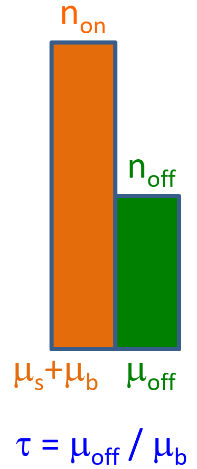
In this simple version discussed here, we assume that the ratio of the Poisson means of background in the two bins, , is precisely known. In astronomy, this could be the ratio of observing times; in HEP, one might rely on simulation or control regions in the data. (If is determined with non-negligible uncertainty from two more control regions, as in the so-called ABCD method in HEP, more issues arise.) In a search for a signal, we test the null hypothesis : , which we can rephrase as : . One can choose the nuisance parameter to be either or , and we choose the latter.
4.1 : conditioning on and using Clopper-Pearson intervals
The standard frequentist solution, invoking “conditioning” (jamesroos; reid1995; CLT), is based on the fact that the total number of counts, , provides information about the uncertainty on the ratio of Poisson means, but no information about the ratio itself. Thus, is known as an ancillary statistic, and most statisticians agree that one should treat as fixed, i.e., calculate (binomial) probabilities of and conditional on the observed . We can again rephrase the null hypothesis in terms of the binomial parameter , namely : . So we do a binomial test of , given data , . The -value is obtained by inversion of binomial confidence intervals.
There are many available choices for sets of binomial confidence intervals. For , CLT adheres to the standard in HEP and follows the “exact” construction of clopper1934, with the guarantee of no undercoverage. Note, however, that “exact”, as commonly used in situations such as this (going back to Fisher), means that a small-sample construction (as opposed to asymptotic theory) was used, but beware that in a discrete situation such as ours, there will be overcoverage, sometimes severe.
The -value is converted to a -value (sometimes called in HEP) with a 1-tailed Gaussian convention to obtain . (As in CLT, .
4.2 : conditioning on and using Lancaster mid-P intervals
After CLT, a paper by myself, Hymes, and Tucker (cht2010) advocated using Lancaster’s mid-P binomial confidence intervals (lancaster61) to obtain confidence intervals for the ratio of Poisson means. For any fixed , the mid-P intervals have over-coverage for some values of the binomial parameter and undercoverage for other values. In the unconditional ensemble that includes sampled from the Poisson distribution with the true total mean, the randomness in leads to excellent coverage of the true ratio of Poisson means.
4.3 : profile likelihood and asymptotic theory
The asymptotic result from Wilks’s Theorem (details in Section 5 of CLT and in pdg2022, Section 5) yields the -value from the profile likelihood function.
4.4 : marginalization of nuisance parameter
(Bayesian-frequentist hybrid)
First, consider the case when is known exactly. The -value (denoted by ) for : is the Poisson probability of obtaining or more events in the “on” bin with true mean .
Then, introduce uncertainty in in a Bayesian-like way, with uniform prior for and likelihood from the Poisson probability of observing in the “off” bin, thus obtaining posterior probability , a Gamma distribution. Finally, take the weighted average of over to obtain the Bayesian-frequentist hybrid -value :
| (6) |
and map to (called by CLT).
Jim Linnemann discovered numerically, and then proved, that (!). His proof is in Appendix C of CLT. This justifies, from a frequentist point of view, the use of the uniform prior for , which is on shaky ground in real Bayesian theory.
The integral in Eq. 6 can be performed using the Monte Carlo method as follows. One samples from the posterior pdf , and computes the frequentist for each sampled value of (using same observed ). Then one calculates the arithmetic mean of these values of to obtain , and converts to as desired. (Note that ’s are averaged, not ’s.)
4.5 : parametric bootstrap for nuisance parameter
For testing : , we first find the profile likelihood estimate of . See lima, cited by CLT, for the mathematics.
Conceptually, we use the data in both bins by noting as above that for , is a sample from Poisson mean . Solving for , the profiled MLE of for is . The parametric bootstrap takes this value of as truth and proceeds to calculate the -value as in above. This can be done by simulation or direct calculation, leading to .
4.6 Numerical examples
The calculated -values for the various recipes are shown in Table 1 for three chosen sets of values of , , and .
Explaining the first set in detail, suppose , , . Following the ROOT commands in Appendix E of CLT yields the “Exact” . Alternatively, one can use the ROOT (tefficiency) class TEfficiency for two-tailed binomial confidence intervals. Recall that we need a one-tailed binomial test of , given data , . Applying the duality between tests and intervals (cousinshcpss2018), we seek the confidence level (CL) of the confidence interval (CI) that just includes the value of . By iterating and the in TEfficiency manually until obtaining the endpoint=0.5 (for ), I arrived at the following ROOT commands (converting to as in CLT).
double n_on=10
double n_off=2
double p=0.019287
endpoint = TEfficiency::ClopperPearson(n_on+n_off,n_on,1.-2.*p,false);
endpoint
Then I could switch to TEfficiency::MidPInterval to get the Lancaster mid-P interval and similarly obtain .
The asymptotic result from Wilks’s Theorem gives the value from the profile likelihood function, .
For the parametric bootstrap, for and , the profiled MLE is , and so . So I generated toys with in each bin (!), to find .
The results for the second set of values (, , and ) are found similarly. For the parametric bootstrap, for , the profiled MLE is , and so . So I generated toys with in the bins where we observed 10, 2 (!). .
The third set of values (added since my talk) has no events in the off sideband, . In the discussion following our talks, I expressed concern about generating toys for the parametric bootstrap in this situation. In fact, it is not a problem. With and , then for and , the profiled MLE is , and so . So I generated toys with in the bins where we observed 6, 0 (!). (In more complicated models, zero events observed in multiple control regions might be an issue.)
| 1.0 | 2.0 | 2.0 | |
| 10 | 10 | 6 | |
| 2 | 2 | 0 | |
| 12 | 12 | 6 | |
| for | 6 | 4 | 2 |
| , Clopper-Pearson | 2.07 | 3.27 | 3.00 |
| , Lancaster mid-P | 2.28 | 3.44 | 3.20 |
| 2.41 | 3.58 | 3.63 | |
| 2.32 | 3.46 | 3.41 |
4.6.1 Discussion
Superficially, given that with Clopper-Pearson intervals is “Exact”, and the parametric bootstrap gives larger , the latter looks anti-conservative. But recall that the so-called “exact” intervals overcover due to discreteness. Maybe is actually better. We need a closer look.
4.7 Coverage studies
Following CLT, we consider a pair of true values of , and for that pair, consider all values of , and calculate both the probability of obtaining that data, and the computed value for each recipe. We consider some threshold value of claimed , say 3 or 5, and compute the probability that according to a chosen recipe; this is the true Type I error rate for that recipe and the significance level corresponding to that value of . One can then convert this true Type I error rate to a -value using the one-tailed formula and obtain what we call . This could be done by simulation, but we do direct calculations. Figure 2 has “heat maps” from CLT showing for claims of 5 for the and profile likelihood algorithms.

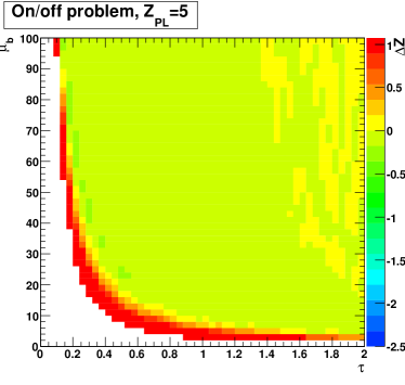
I calculated a couple of points using the parametric bootstrap : For , , and , I found (!) For , , and , I found (!) Thus, at least for these two points, any anti-conservatism of the parametric bootstrap is exactly canceled out by the over-coverage due to discreteness. That is, I cherry-picked my example problem to be one in which I knew that marginalizing the nuisance parameter (with judicious prior) yielded the standard frequentist , while doing parametric bootstrap as commonly done at the LHC would give higher . But in this example, the discrete nature of the data in the problem “saves” the coverage of !
Note also the similarity of with . As mentioned, cht2010 found that Lancaster mid-P confidence intervals had excellent coverage in the unconditional ensemble, i.e., not conditioning on .
4.8 If is not known exactly
An obvious next step is to relax the assumption that is known exactly, so that becomes a nuisance parameter. In analyses in HEP, is often estimated from the observed data in two so-called control regions (bins), which are thought to have the same ratio of background means as the original two bins. The control regions are distinguished from the original two bins by using an additional statistic that is thought to be independent of the statistic used to define the original two bins. This is often referred to as the ABCD method, after the letters commonly designating the four bins. I would strongly encourage coverage studies for the various methods applied to this case. One could also study the case where the estimate of is sampled from a lognormal distribution.
5 Discussion at Banff BIRS 2023
Among the many talks touching on the topic at Banff in davisonbanff2023, statistician Anthony Davison’s was paired with mine, pointing to works including his Banff challenge paper with Sartori, and describing a parametric bootstrap, writing,
“Lee and Young (2005, Statistics and Probability Letters) and DiCiccio and Young (2008, 2010, Biometrika) show that this parametric bootstrap procedure has third-order relative accuracy in linear exponential families, both conditionally and unconditionally, and is closely linked to objective Bayes approaches.”
6 Final remarks
Overall, I am encouraged by what I learned in the last year while preparing the talks and this writeup regarding our widespread use of the parametric bootstrap with the PLR test statistic in HEP. Still, there is room to learn more (which I suspect that I must leave to the younger generations). First, how much is HEP losing by not studying more thoroughly the higher-order asymptotic theory in the test statistic? Would that give more power, or at least reduce the need for parametric bootstrapping? Second, can one find relevant cases in HEP where marginalizing out-performs profiling? Is there an example having continuous data but otherwise similar to the example in this note, so that one can study the performance without the confounding complication of discreteness? Or, for those familiar with the ABCD method in HEP (where, as mentioned) is measured from contents of two more control regions), are there pitfalls for the parametric bootstrap in that context? I would urge more exploration of these issues in real HEP analyses!
Acknowledgments
Many thanks go to the multitudes of physicists and statisticians from whom I have learned, and particularly to Louis Lyons for bringing us together regularly at PhyStat meetings since the year 2000 (and for comments on earlier drafts). I also thank him, Sara Algeri, and Olaf Behnke for organizing this discussion. This work was partially supported by the U.S. Department of Energy under Award Number DE–SC0009937.
Part II: Statistician’s View
by Larry Wasserman
1 Introduction
This paper arose from my presentation at the PhyStat meeting where Bob Cousins and I were asked to give our views on two methods for handling nuisance parameters when conducting statistical inference. This written account expands on my comments and goes into a little more detail.
I’ll follow Bob’s notation where is the (real-valued) parameter of interest and is the vector of nuisance parameters. In his paper, Bob points out that marginalising nuisance parameters is rare at the LHC. This is true in statistics as well. There are a few cases where marginalising is used, such as random effects models where the number of parameters increases as the sample size increases. But even profile likelihood is not that common. I would say that the most common method in statistics is the Wald confidence interval where is the maximum likelihood estimator, is the standard error (usually obtained from the Fisher information matrix) and is the upper quantile of a standard Normal distribution. (Note that for the Wald interval, one simply inserts points estimates of the nuisance parameters in the formula for .)
Let be a random sample from a density which belongs to a model . We decompose the parameter as where is the parameter of interest and is a vector of nuisance parameters. We want to construct a confidence set such that
| (7) |
or, equivalently,
We may also want to test
however, for simplicity, I’ll focus on confidence sets. The present discussion is on likelihood based methods. In particular, we may use the profile likelihood
or the marginalised (or integrated) likelihood
where is a prior for . In my view, we cannot say whether a likelihood is good or bad without saying what we will do with the likelihood. I assume that we are using the likelihood to constructing confidence intervals and tests. Then judging whether a likelihood is good or bad requires assessing the quality of the confidence sets obtained from the likelihood. The usual central confidence set based on is
| (8) |
where is the maximum likelihood estimate, and is the quantile of a distribution.
2 Profile or Marginalise?
We want confidence intervals with correct coverage which means that for all . In this case we say that the confidence set is valid. Among valid intervals, we may want one that is shortest. A valid interval with shortest length is efficient. (But this is a scale dependent notion.)
If the sample size is large and certain regularity conditions hold, then the profile-based confidence set in (8) will be valid and efficient. So in these well-behaved situations, I don’t see any reason for using . The main regularity conditions are:
(1) is a smooth function of .
(2) The range of the random variable does not depend on .
(3) The number of nuisance parameters does not increase as the sample size increases.
In a very interesting paper that Bob mentions, berger1999 provide examples where apparently does not behave well. This is because, in each case, the sample size is small, or the number of nuisance parameters is increasing or some other regularity conditions fail. There may be a few cases where the marginalised likelihood can fix these things if we use a carefully chosen prior, but such cases are rare. We might improve the accuracy of the coverage by using higher order asymptotics. But this is rarely done in practice. Such methods are not easy to apply and they won’t necessarily help if there are violations of the regularity conditions.
Sometimes we can use specific tricks, like conditioning on a well-chosen statistic as Bob does in the Poisson ON-OFF example. These methods are useful when they are available but they tend to be very problem specific. Bootstrapping and subsampling are also useful in some cases. A common misconception is that the bootstrap is a finite sample method. It is not. These methods are asymptotic and they do still rely on regularity conditions.
In the next two sections I’ll discuss two approaches for getting valid confidence sets without relying on asymptotic approximations or regularity conditions.
3 Universal Inference
Universal inference (wasserman2020universal) is a method for constructing confidence sets from the likelihood that does not rely on asymptotic approximations or on regularity conditions. The method, works as follows.
-
1.
Choose a large number .
-
2.
For :
-
(a)
Split the data into two disjoint groups and .
-
(b)
Let be any estimate of using .
-
(c)
Let where is the likelihood constructed from .
-
(a)
-
3.
Let .
-
4.
Return .
This confidence set is valid, that is,
and this holds for any sample size. It does not rely on large sample approximations and it does not require any regularity conditions. The number of splits can be any number, even is allowed. The advantage of using large is that it removes the randomness from the procedure. The disadvantage of Universal inference is that one needs to compute the likelihood many times which can be computationally expensive.
4 Simulation Based Inference
As the name implies, simulation based inference (SBI) uses simulations to conduct inference. It is usually used to deal with intractable likelihoods (dalmasso2021likelihood; masserano2023simulator; al2024amortized; cranmer2015; cranmer2020; thomas2022; xie2024; masserano2022simulation; stanley2023). But it can be used as a way to get valid inference for any model. The idea is to first get a confidence set for by inverting a test. Let denote the true value of . For each we test the hypothesis . This test is based on some test statistic . The p-value for this test is
where . Then is an exact, confidence set for . The confidence set for is the projection
Such projected confidence sets can be large, but the resulting confidence sets have correct coverage. In SBI, we sample a set of values from some distribution. For each we draw a sample . Then we define
which is 1 if and 0 otherwise. Note that
So is an unbiased estimate of . But we can’t estimate using a single observation . Instead, we perform a nonparametric regression of the ’s which allows us to use nearby values. For example we can use the kernel regression estimator
where is a kernel with bandwidth such as . Here are the steps in detail.
-
1.
Choose any function .
-
2.
Draw from any distribution with full support. This can be the likelihood but it can be anything.
-
3.
For : draw and compute .
-
4.
Let for . Here, if and otherwise.
-
5.
Estimate by regressing on to get .
-
6.
Return: .
We have that as . The test statistic can be anything. A natural choice is the likelihood function . In fact, even if the likelihood is intractable it too can be estimated using the simulation. See (dalmasso2021likelihood; masserano2023simulator; al2024amortized; cranmer2015; cranmer2020; thomas2022) for details. A related method is given in xie2022.
5 Optimality
Suppose we have more than one valid method. How do we choose between them? We could try to optimize some notion of efficiency. For example, we could try to minimize the expected length of the confidence interval. However, this measure is not transformation invariant so one has to choose a scale. The marginalised likelihood could potentially lead to shorter intervals if the prior happens to be concentrated near the true parameter value but, in general, this would not be the case. (hoff2022 discusses methods to include prior information while maintaining frequentist coverage guarantees.) For testing, we usually choose the test with the highest power. But generally there is no test with highest power at all alternative values. One has to choose a specific alternative or one puts a prior on and maximizes the average power.
Again, in the large sample, low dimension regime the choice of procedure might not have much practical impact. In small sample size situations, careful simulation studies are probably the best approach to assessing the quality of competing methods.
Of course, there may be other relevant criteria such as simplicity and computational tractability. These need to be factored in as well.
6 Why Likelihood?
There are cases where neither the profile likelihood or the marginalised likelihood should be used. Here is a sample example. Let be a set of fixed, unknown constants such that . Let . Let be independent flips of a coin where . If you get to see . If then is unobserved. Let
Then and a simple confidence interval for is . The likelihood is the probability of coin flips which is which does not even depend on . In other words, the likelihood function is flat and contains no information. What’s going here? The variables are ancillary which means their distribution does not depend on the unknown parameter. Ancillary statistics do not appear in the likelihood. But the estimator above does use the ancillaries which shows that the ancillaries contain valuable information. So likelihood-based inference can fail when there are useful ancillaries. This issue comes up in real problems such as analyzing randomized clinical trials where the random assignment of subjects to treatment or control is ancillary.
Another example is Example 7 from berger1999. Let and suppose that the parameter of interest is . berger1999 shows that both profile and marginalised likelihood functions have poor behavior. But there is no need to use either. We can define a confidence set where is a joint confidence set for . This is a valid confidence set which uses neither or .
In some cases, we might want to use semiparametric methods instead of likelihood based methods. Suppose, for example, that the nuisance parameter is infinite dimensional. For example, consider testing for the presence of a signal in the presence of a background. The data take the form
where , is a known background distribution and is the signal. Suppose that is supported on a signal region but is otherwise not known. We want to estimate or test . The unknown parameters are . Here, is any density such that . So is an infinite dimensional nuisance parameter. In our previous notation, the parameter of interest is and the nuisance parameter is .
Models of this form might be better handled using semiparametric methods (tsiatis2006; kosorok2008). It is hard for me to judge whether such methods are useful in physics but they may indeed be cases where they are. The main idea can be summarized as follows. Suppose that is the parameter of interest and is the (possibly infinite dimensional) nuisance parameter. Any well-behaved estimator will have the property that will converge to a Normal with mean 0 and some variance . Generally, for a function which is known as the efficient influence function. We then try to find so that its corresponding is equal to . Such an estimator is said to be semiparametric efficient.
In our signal detection example, the efficient influence function is
where and the efficient estimator is simply
The point is that we have taken care of an infinite dimensional nuisance parameter very easily and we never mentioned likelihood.
Another reason to consider non-likelihood methods is robustness. Both the profile likelihood and the marginalised likelihood could lead to poor inferences if the model is misspecified. What should we do in such cases? One possibility is to use minimum Hellinger estimation. In this case we choose to minimize
where is some non-parametric density estimator. This estimator is asymptotically equivalent to the maximum likelihood estimator if the model is correct but it is less sensitive to model misspecification (beran1977; lindsay1994).
Another recent non-likelihood method is the HulC (hulc). We divide the data into disjoint groups. Let be estimates from the groups and let . Define the median bias
So . In the extreme situation where is larger than the true value with probability 1, we have . Otherwise . If as is typically the case, we have . This is simple and does not require profiling or marginalising a likelihood function.
7 Conclusion
The confidence intervals and tests based on the profile likelihood should have good coverage and reasonable size as long as the sample size is large, the number of nuisance parameters is not too large and the usual regularity conditions hold. If any of these conditions fail to hold, it might be better to use alternative methods such as Universal inference, simulation based inference, semiparametric inference or the HulC. The integrated likelihood may offer benefits in some special cases but I don’t believe it is useful in any generality.
I conclude with remarks about power. Methods like Universal inference, SBI and the HulC give satisfying coverage guarantees but these come with some loss of efficiency. The confidence sets from Universal inference typically shrink at the optimal rate but will nonetheless be larger than optimal confidence sets (if such optimal sets exist). As a benchmark, consider the confidence set for where . Of course we don’t need Universal inference here but this case allows for precise results. dunn2023 show that the confidence set has radius of order which is optimal but, compared to the best confidence set the squared radius is about twice as large. More precisely, the ratio squared radii is bounded by . Similarly, comparing the HulC to the Wald interval (when the latter is valid) we find that the length is expanded by a factor of which is quite modest. For SBI it is hard to say much since that method works with any statistic and the size of the set will depend on the particular choice of . However, it is fair to say that using generally applicable methods that provide correct coverage under weak conditions, there will be some price to pay. Evaluating these methods in some real physics problems would be very valuable. This would be a great project for statisticians and physicists to collaborate on.
8 Acknowledgments
Thanks to Sara Algeri, Louis Lyons and Olaf Behnke for organizing this discussion. Also, I would like to thank Louis Lyons and Bob Cousins for comments on an earlier draft that led to improvements in the paper.