Optimizing Cycle Life Prediction of Lithium-ion Batteries via a Physics-Informed Model

Abstract

Accurately measuring the cycle lifetime of commercial lithium-ion batteries is crucial for performance and technology development. We introduce a novel hybrid approach combining a physics-based equation with a self-attention model to predict the cycle lifetimes of commercial lithium iron phosphate graphite cells via early-cycle data. After fitting capacity loss curves to this physics-based equation, we then use a self-attention layer to reconstruct entire battery capacity loss curves. Our model exhibits comparable performances to existing models while predicting more information: the entire capacity loss curve instead of cycle life. This provides more robustness and interpretability: our model does not need to be retrained for a different notion of end-of-life and is backed by physical intuition.

Keywords— electric vehicles, state of health, Arrhenius law, discharge voltage curve, self-attention, multi-stage training

1 Introduction

Predicting the cycle life of a lithium-ion battery remains challenging due to the complexity of the chemical side effects responsible for degrading the performance of a battery as it is repeatedly cycled. In particular, it is well known that solid electrolyte interphase (SEI) formation crucially affects cycle life and occurs within the first few charging/discharging cycles [17, 18, 13, 3]. Accurately predicting the cycle life of batteries while accounting for all these side chemical processes is important for maintaining battery performance.

Recently, Severson et al. [12] presented a state-of-the-art dataset containing $124$ lithium-ion batteries with $72$ different fast-charging policies and showed that a regularized linear regression model predicting cycle lifetimes performs very well on batteries with different charge policies. They also successfully showed that this prediction can be obtained within the first hundred charging cycles. Their method of using early-cycle data for prediction has great practical implications, since one need not wait to charge a battery for many cycles before knowing its lifetime.

Previous literature on predicting cycle lifetimes of batteries is rich. Data-driven models [25, 4, 2, 21], which focus on using machine learning techniques to identify trends in how batteries degrade, have been thoroughly studied, with models ranging from linear models [12] to neural networks [4, 14, 15] to support vector regression [26]. These types of models are agnostic to the mechanisms of degradation, but they can be difficult to fine-tune. Physics-based models, which rely upon knowledge in how a battery degrades over time, have also been well-studied. These methods usually rely upon cell chemistry [19, 10, 24] or analyzing how the material in the electrodes changes over time [5, 9]. However, since batteries can be charged/discharged in a variety of environments, this hinders how descriptive physical models by themselves can be. Recently, hybrid models combining physics knowledge with a data-driven approach have been proposed [22, 6, 8, 11] to combine the advantages of both approaches.

We propose a hybrid model combining a physics-based equation and a self-attention mechanism for prediction. The latter is inspired by the recent rise of transformers to predict sequential data [7, 16], and the former uses physics insights to capture more information on the behavior of the capacity loss curves of lithium-ion batteries. Although transformers have already found applications in predicting the cycle life of batteries [23], combining a physical equation with self-attention to predict complete capacity loss curves has not been thoroughly studied to the best of our knowledge.

The paper is organized as follows. In Section 2 we introduce data processing techniques and extract relevant information from discharge curves. We then introduce a hybrid model utilizing an Arrhenius Law to model capacity loss and utilize self-attention to predict cycle life from early-cycle discharge data. Finally, we compare our errors with Severson et al. [12] and conclude with future directions.

2 Data Processing

We utilize the public dataset provided by Severson et al. [12]. This dataset comprises 124 lithium-ion phosphate/graphite battery cells, each with a nominal capacity of 1.1 ampere-hours (Ah) [1]. The cells are cycled (repeatedly charged/discharged) until end of life, which is defined as the point where the effective capacity of the battery has dropped to 80% of its nominal value. The ratio of the effective and nominal capacity is commonly referred to as the state of health. All battery cells in this dataset are cycled under fast-charging conditions in a constant-temperature environment; however, the charging policy dictating the specific charge rate schedule differs from cell to cell.

In our work, we preserve the train/test/secondary test data split in Severson et al. [12], allowing for a direct comparison between our result and theirs. The primary test set was obtained using the same batch of cells as the train set and similar charge policies, therefore we use it to evaluate the model’s ability to interpolate in the input space. On the other hand, the secondary test set was obtained from a different batch of cells and using significantly different scheduling, and we use it to examine the model’s ability to extrapolate. Ensuring our model can generalize to different batteries makes for an advantage over prior work [11, 14] that uses a random split of cells into train/validation/test sets.

For each cell, three forms of data are recorded:

1. Cycle life: The number of charge/discharge cycles until the state of health drops to 80%, ranging from 150 to 2,300.

2. Charge policy: The schedule of charge rates followed during cell cycling.

3. Cycle summary features: Features calculated for each cycle, such as the state of health, internal resistance ($IR$), average cell temperature ($T_{\text{avg}}$), and maximum cell temperature ($T_{\text{max}}$).

4. Full cycle data: Measurements taken over the course of each cycle, such as voltage ($V$), discharged capacity ($Q_{d}$), and temperature ($T$).

Voltage ($V$) and discharged capacity ($Q_{d}$) are particularly relevant for lifetime prediction and are depicted for an example charge-discharge cycle in Figure 1(a).

The discharge-voltage curve for a cycle, denoted $Q_{d}(V)$, is constructed by plotting $Q_{d}$ against $V$ for the discharge portion of the cycle, as boxed in Figure 1(a). One such curve is shown in Figure 1(b). According to manufacturer specifications, a battery cell is considered fully charged when its voltage reaches 3.6V and fully discharged when it reaches 2.0V [1]. An analogous curve can be constructed for each cycle of a battery’s operation.

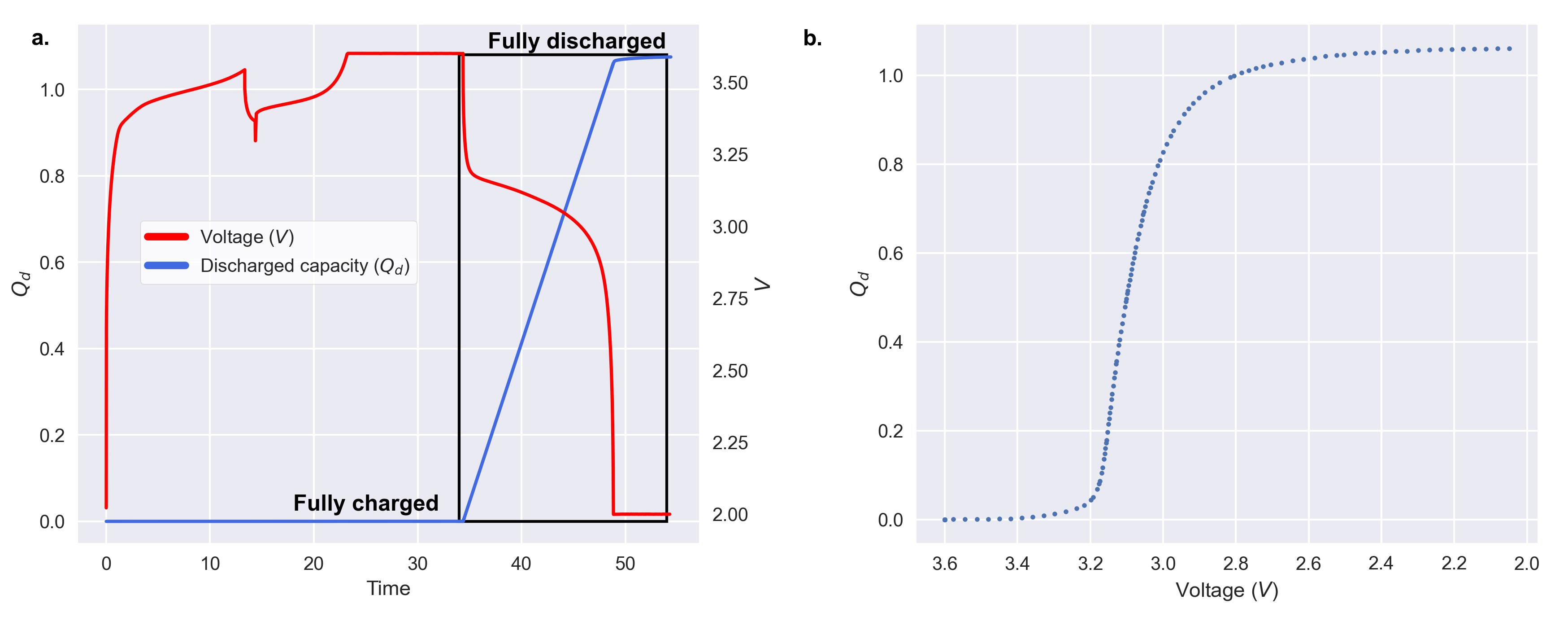
Figure 1: (a) Discharged capacity, $Q_{d}(t)$, and voltage, $V(t)$, measured for one battery over the course of a charge-discharge cycle. The discharge portion of the cycle is boxed in black. (b) The discharge-voltage curve, $Q_{d}(V)$, for the same battery. N.B.: the x-axis in (b) is flipped to reflect voltage decreasing over the course of the discharging process.

Choosing the voltage to be our $x$ coordinate for the discharge curves rests in a highly irregular set of evaluation points for $Q_{d}(V)$. As illustrated in Figure 1(b), the $V$ values sampled at regular timesteps are sparser in the intervals $[3.2\text{V},\,3.6\text{V}]$ and $[2.0\text{V},\,3.0\text{V}]$ and denser in the interval $[3.0\text{V},\,3.2\text{V}]$. Moreover than being irregular, the points at which $Q_{d}(V)$ were to be evaluated are also different from one cycle to another. This makes direct comparisons between different cycles difficult. To standardize the discharge curves, we utilize radial basis function interpolation, a standard method used for irregularly spaced inputs (Supplementary Text 1). In 1D, this consists of an interpolant given by Equation 1:

$$\hat{Q}_{d}(V)=p_{m}(V)+\sum_{i=1}^{N}\lambda_{i}\phi(|V-V_{i}|)$$ (1)

The datapoints are therefore interpolated by a weighted sum of radial basis functions, with the origins at the interpolation nodes $V_{i}$, and by $p_{m}(V)=c_{0}+c_{1}V+\dots+c_{m}V^{m}$, a polynomial of degree $m$. The coefficients of $p_{m}$ and the weights $\lambda_{i}$ are found by solving a set of linear equations. The form of $\phi$ dictates the final form of the interpolant. The role of the polynomial term is to model any possible trend in the data, which the RBFs are unable to do due to their symmetric, radial nature.

Evolution of $Q_{d}(V)$ over cycles can be exploited to predict battery lifetime. Severson et al. [12] observe that more dramatic early-cycle curve sagging occurs for batteries with low lifetimes than for batteries with high lifetimes, as visualized in Figure 2(a, b). To capture the phenomenon of curve sagging, Severson et al. propose taking the discharge-voltage curves for cycles 100 and 10 and computing the difference between the two. This new curve, calculated as $Q_{d,100}(V)-Q_{d,10}(V)$, is denoted $\Delta Q_{100-10}(V)$. Figure 2(c,d) shows that $\Delta Q_{100-10}(V)$ succinctly capture the difference in curve sagging behavior between two batteries of different cycle lives, and Figure 2(e) shows a clear linkage between curve shape and cycle life across all batteries in the dataset. In particular, batteries with shorter cycle lives exhibit more ample dips in the $\Delta Q_{100-10}(V)$ curve.

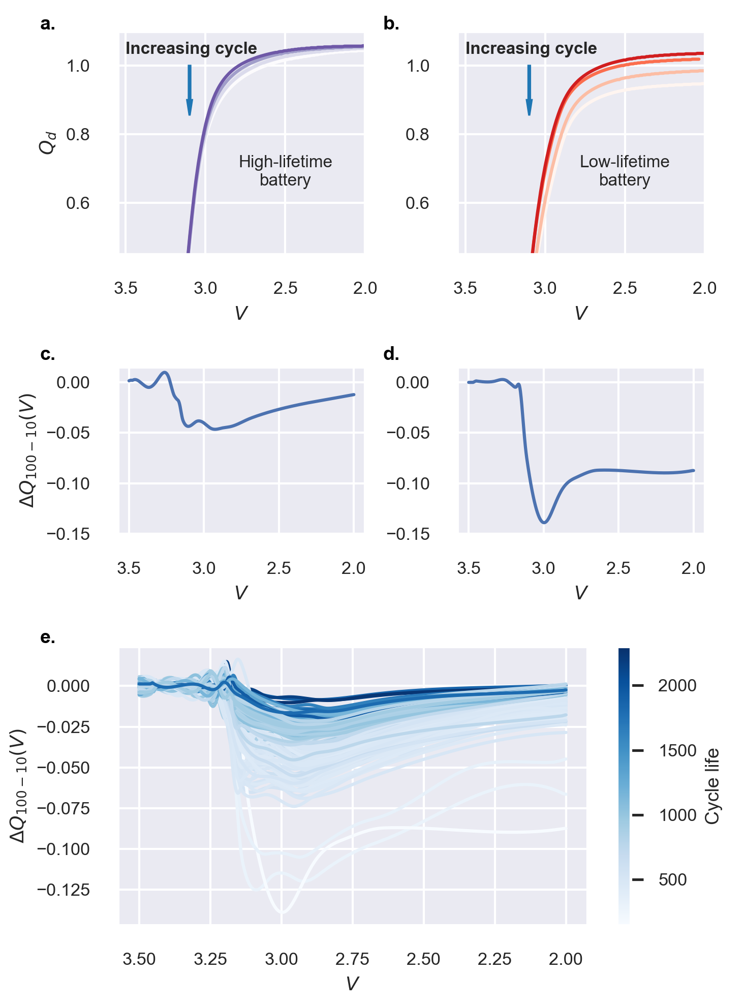
Figure 2: (a, b) Evolution of the discharge-voltage curve over cycles for two batteries with different cycle lives. Curves from cycles evenly spaced between 1 and 100 are plotted and distinguished by saturation. As cycle number increases, the curve progressively sags more for the battery with lower lifetime. (c, d) $\Delta Q_{100-10}(V)$ for the same two batteries. (e) $\Delta Q_{100-10}(V)$ plotted for all batteries in the dataset, with shade corresponding to cycle life.

Now statistical quantities, such as the variance, minimum, and mean, of $\Delta Q_{100-10}(V)$ are calculated to further condense information of cycle life for each battery. A simple variance-based model would, for instance, use $\text{Var}(\Delta Q_{100-10}(V))$ as an input to predict the cycle life for a single battery.

3 Model

3.1 Physics-Based Model

It is well known that as a lithium-ion battery is cycled, other chemical processes occur in the battery that affects long term cyclability. Notably, the SEI (solid electrode interphase) is formed on the surface of the anode within the first five charging cycles, impeding electron movement in the battery. Although poorly understood, it is believed that SEI formation has an impact on capacity loss [17]. Hence it is important to consider the impact of SEI formation when studying capacity loss. In response, we construct a model of the capacity curves in the Severson et al. dataset via an Arrhenius Law, which is commonly associated with chemical processes akin to SEI formation [18, 13, 3].

We now introduce an equation describing the process of capacity loss. Wang et al. (2011) [18] have shown that for different charge rates, the true capacity loss $Q_{\text{loss}}$ can be approximated as

$$\hat{Q}(x)_{\text{loss}}=B\exp\left(-\frac{E_{a}}{RT}\right)x^{z}$$ (2)

for constants $B$ and $z$, where $\hat{Q}_{\text{loss}}$ represents the percentage of capacity loss, $E_{a}$ is the activation energy, $R$ the gas constant, $T$ the absolute temperature, and $x$ the cycle number. Note that the temperature highly resembles an Arrhenius Law, which is commonly associated with a thermally activated chemical process, such as SEI layer formation during cycling [18, 13, 3]. Equation (2) accounts for SEI formation that produces undesired side effects in batteries. In addition, there is also a power law with respect to the cycle number, consistent with previous findings of the rate of lithium consumption at the negative electrode [18, 13, 20, 3]. In short, this equation accounts for SEI formation and is consistent with the resulting mechanism of active lithium consumption in the presence of the SEI layer.

We adapt Equation (2) in three ways. Firstly, we noticed that typical values of the constant $B$ are found to have a very large order of magnitude, which introduces numerical instability and overflow issues in further calculations. We mitigate this by predicting $\ln B$ instead of $B$ itself. Secondly, the average temperatures reached during testing did not vary greatly across cycles. Treating $T$ as invariant allows us to incorporate the original exponential factor from Equation (2) into the previously described constant. This has the subtle advantage that $E_{a}$ need not be known anymore.

We lastly adopt the addition of a constant $C$ by shifting up the predicted curves such that their first point matches the first point of the ground truth capacity loss curve. Specifying such constant reduces one free variable and makes fitting easier. Thus, we may reduce Equation (2) to one of the form

$$\hat{Q}(x)_{\text{loss}}=e^{A}x^{B}+Q(0).$$ (3)

We then fit Severson et al’s capacity loss curves with equations of the form in Equation (3) via least squares regression. Figure 3(a-c) illustrates three capacity loss curves with substantially different cycle lives and their best fit curves. Not only are the curves themselves a good fit, but the cycle lives as predicted by our best fit curves are remarkably similar to the actual cycle lives. Cycle life $\ell$ is the point where $\hat{Q}_{\text{loss}}(\ell)=0.2$, calculated from the best fit curve as

$$\ell=[e^{-A}(0.2-Q(0))]^{1/B},$$ (4)

where 0.2 is used as the threshold capacity loss indicating end of life. Figure 3d plots true cycle life against predicted cycle life for all batteries in the dataset and demonstrates high goodness of fit, with $R^{2}=0.994$ and a RMSE of 28.6.

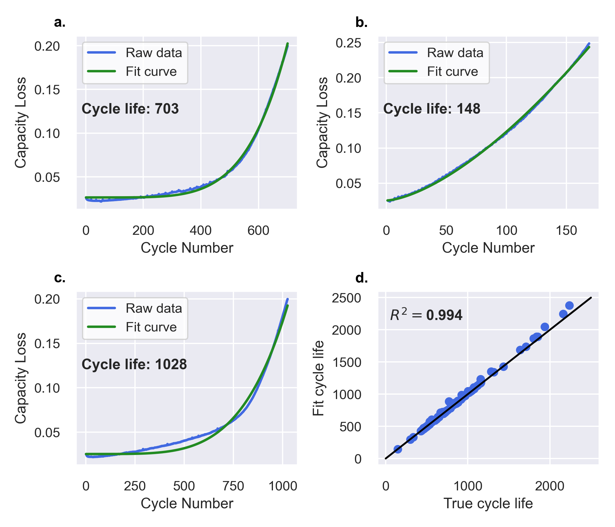
Figure 3: (a-c) Capacity loss model fit to three capacity loss curves using least-squares. The three curves reflect batteries with substantially different lifetimes, demonstrating the ability of the model to generalize. $R^{2}$ for each individual battery is displayed, and average $R^{2}$ across all 124 batteries in the dataset is 0.976. (d) Cycle lives derived from the fitted capacity loss curves, plotted against true cycle lives. We observe $R^{2}=0.994$, demonstrating high goodness of fit.

As seen in Figure 3(d), our equation very accurately models the cycle lives of batteries, and henceforth we assume that the ground truth of capacity loss follows Equation (3), given values of $A$ and $B$. In other words, we assume that our predicted $\hat{Q}_{\text{loss}}\approx Q_{\text{loss}}$. Hence the second half of our hybrid model involves training a self-attention model to predict $\hat{A}$ and $\hat{B}$ from cycle input data of the first 100 cycles. Call this model $f$. Then given a vector $\mathbf{x}$ of early-cycle statistical quantities, our output variables are $(\hat{A},\hat{B})=f(\mathbf{x})$ and our predicted cycle life is $\hat{\ell}=[e^{-\hat{A}}(0.2-C)]^{1/\hat{B}}$. This model is illustrated in Figure 4.

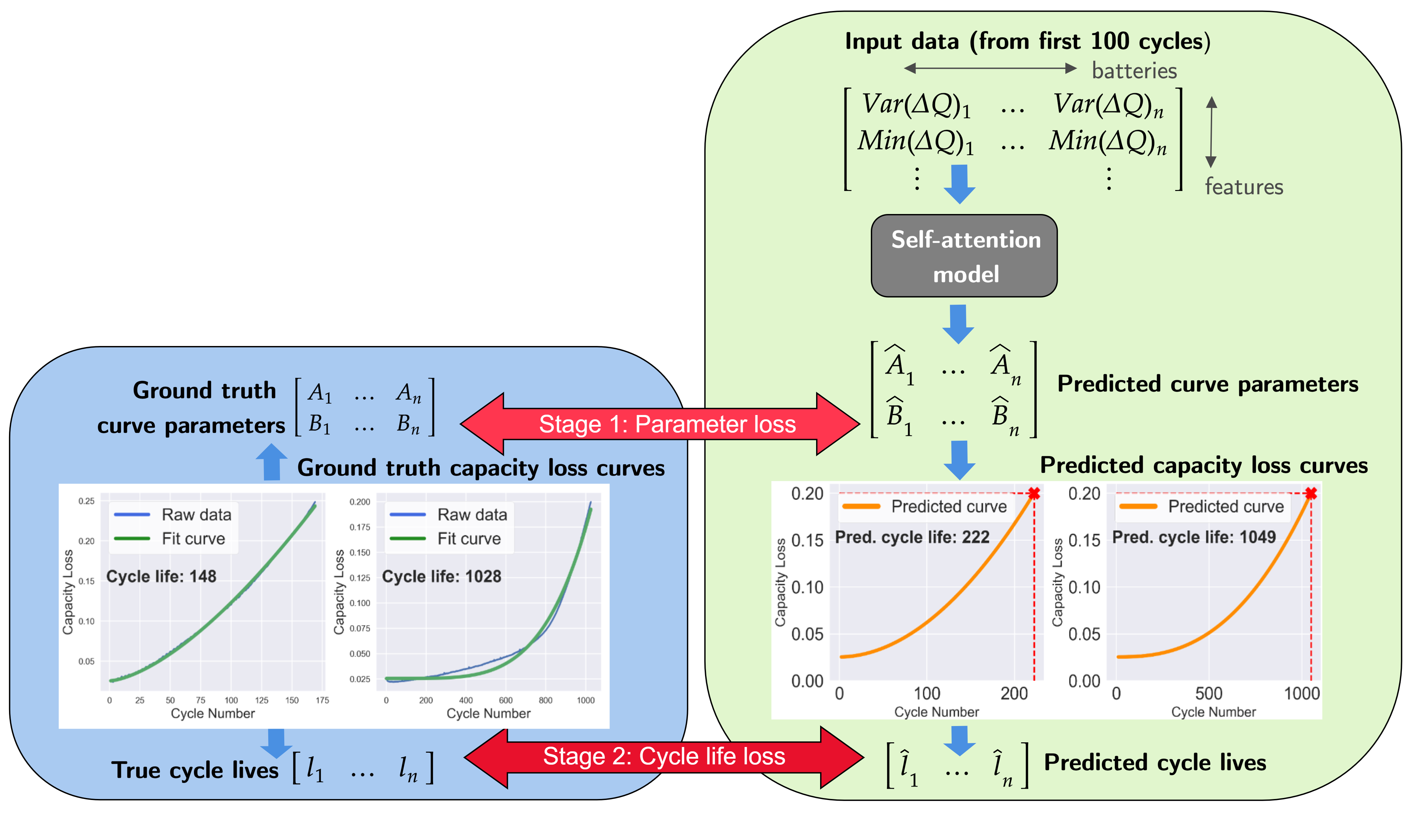
Figure 4: Schematic of the physics-based model. One half utilizes an Arrhenius Law-inspired model to capture capacity loss curves. The other half utilizes self-attention to predict Arrhenius Law parameters from early-cycle data.

3.2 Self-Attention for Regression

We endeavor to predict the parameters of the capacity loss curve based on early-cycle data, when the full capacity loss curve is not known. When limited to early-cycle capacity loss data, we cannot fit and extrapolate the full curve with good fidelity using least squares. Instead, we employ a self-attention mechanism to learn complex, nonlinear relations between the capacity loss curve and other measurements available during a battery’s early operation. As presented in [7], there exists an equivalence between the self-attention mechanism and a support vector regression (SVR) problem formulation. This implies that any problem where an SVR model performs well can potentially be improved by employing an attention-based architecture.

Let the input sequence of $N$ features derived from early-cycle operation data for the $i$-th battery be denoted $\mathbf{x_{i}}:=[x_{i}^{(1)},\dots,x_{i}^{(N)}]^{T}\in\mathbb{R}^{N\times 1}$. We compute the standard query matrix Q, key matrix K, and value matrix V from the self-attention mechanism via the following transformations:

$$\mathbf{Q}_{i}=\mathbf{x}_{i}\mathbf{W}^{T}_{Q}$$

$$\mathbf{K}_{i}=\mathbf{x}_{i}\mathbf{W}^{T}_{K}$$

$$\mathbf{V}_{i}=\mathbf{x}_{i}\mathbf{W}^{T}_{V},$$

where weight matrices $\mathbf{W}_{Q}$, $\mathbf{W}_{K}\in\mathbb{R}^{D\times 1}$ and $\mathbf{W}_{V}\in\mathbb{R}^{D_{v}\times 1}$ are learnable layers, $D$ is a hyperparameter determining the embedding dimension, and $D_{v}$ is the output dimension. Note that for the multi-output regression task of predicting two variables, $D_{v}=2$. We define the self-attention output $\mathbf{H}_{i}$ as:

$$\mathbf{H}_{i}=softmax\left(\frac{\mathbf{Q}_{i}\mathbf{K}_{i}^{T}}{\sqrt{D}}\right)\mathbf{V}_{i}:=\mathbf{A}_{i}\mathbf{V}_{i}$$

where the softmax function above is applied to each row of the matrix $\frac{\mathbf{Q}_{i}\mathbf{K}_{i}^{T}}{\sqrt{D}}$ to obtain the attention matrix $\mathbf{A}_{i}$. To collapse the output $\mathbf{H}_{i}\in\mathbb{R}^{N\times D_{v}}$ to a vector, we append an averaging layer to the self-attention mechanism that takes the mean along the columns of $\mathbf{H}_{i}$:

$$\mathbf{y}_{i}:=\mathbf{H}_{i}^{T}\mathbf{m}=\begin{bmatrix}\hat{A}_{i}\\ \hat{B}_{i}\end{bmatrix}$$

where $\mathbf{m}=[\frac{1}{N}\dots\frac{1}{N}]^{T}\in\mathbb{R}^{N\times 1}$. The result $\mathbf{y}_{i}\in\mathbb{R}^{D_{v}\times 1}$ is the vector of predicted parameters for the capacity loss curve. These parameters are then used to predict cycle life:

$$\hat{l_{i}}=[e^{-\hat{A}_{i}}(0.2-C_{i})]^{1/\hat{B}_{i}}.$$ (5)

3.3 Feature Selection

Finally, we select the best features for prediction. In Supplementary Table 1, we list all the features we obtain from the charge and discharge curves as explained in Section 2. Our main task is to carefully select the features that are most closely related to our target variables, $\hat{A}$ and $\hat{B}$. To accomplish this, we analyze the correlation between each feature and the target variables. We prioritize features with strong positive or negative correlations, as they are more likely to provide accurate predictions.

We use Spearman’s correlation coefficient to ascertain which features are most correlated with $\hat{A}$ and $\hat{B}$. Spearman’s correlation coefficient is a statistical measure that assesses the strength and direction of the monotonic relationship between two variables. It is particularly useful when the relationship between variables is nonlinear. In our analysis, we select the top five features with the highest correlation coefficients. The results of our correlation analysis using this approach are visually represented in Figure 5. Note that these features are DeltaQ_logVars, DeltaQ_logMin, DeltaQ_logMean, slope_capacity_fade_2_100, and slope_capacity_91_100. These five features were used to train the self-attention model as explained in Section 3.2.

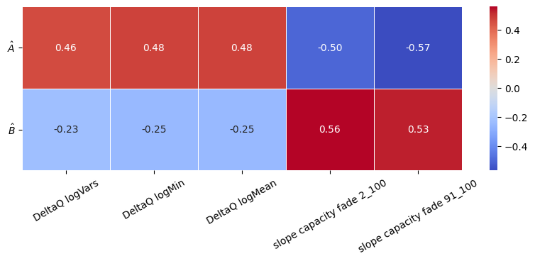
Figure 5: Feature correlation of the selected features with equation parameters.

3.4 Model Training

Our interest lies in minimizing the root mean squared error (RMSE) of cycle life predictions, defined for a set of $n$ batteries as:

$$\text{RMSE}_{l}=\sqrt{\frac{1}{n}\sum_{i=1}^{n}(l_{i}-\hat{l}_{i})^{2}},$$ (6)

where $l_{i}$ is the true cycle life of the $i$-th battery. However, given the complexity of the expression for cycle life, attaining optimal convergence is a nontrivial numerical task. To this end, we employ a two-stage procedure of coarse training on curve parameters followed by fine-tuning on cycle life.

In the first stage, we train on the RMSE of parameter loss, defined as

$$\text{RMSE}_{p}=\sqrt{\frac{1}{n}\sum_{i=1}^{n}\left(w_{A}(A_{i}-\hat{A}_{i})^{2}+w_{B}(B_{i}-\hat{B}_{i})^{2}\right)}.$$ (7)

where $w_{A}$ and $w_{B}$ are tunable hyperparameters. The parameter loss function is smoother and leads to fewer numerical issues than Equation (6), producing stable results when training from a random initialization. In contrast, we observe that training only with the cycle life loss function leads to exploding gradients and inconsistent behavior.

However, parameter loss is not always indicative of the accuracy of cycle life predictions. Due to the high nonlinearity of the capacity loss curve, it is possible for two sets of parameter estimates to incur equal parameter loss but produce dramatically different cycle life predictions (Supplementary Figure 1). Consequently, we follow up coarse training with a fine-tuning stage under low learning rate that trains on cycle life loss.

The two-stage training procedure can be summarized as follows:

1. Coarse training on parameter loss (Equation (7)). This stage guides the model from a random initialization toward approximate parameters, eliminating numerical issues that would otherwise occur in Stage 2.

2. Fine-tuning on cycle life loss (Equation (6)). As many combinations of $\hat{A}$ and $\hat{B}$ can lead to similar parameter losses, this stage tunes the approximate parameters from Stage 1 to produce the most accurate cycle life predictions.

The choice of optimal hyperparameters are based upon the existing literature, and such parameters can be consulted in the Github repository associated with our work, available upon request.

4 Results

We initiate the model training phase with a basic regularized linear framework. The baseline model is similar to the model that performed the best in Severson et al.’s findings and utilizes sklearn’s ElasticNet model [12]. For hyperparameter tuning, we vary alpha and l1_ratio on a logscale over $10^{0}$ and $10^{1}$ and $10^{-5}$ and $10^{2}$, respectively. We find that the best model had a primary test RMSE of 398.98 cycles and a secondary test RMSE of 455.4 cycles.

The results of our model evaluation are presented in Figure 6. We compare the performance of the elastic net baseline with that of the self-attention model in terms of train RMSE, primary test RMSE, and secondary test RMSE. Results from the self-attention model are divided into two stages, Stage 01 and Stage 02, corresponding to the two phases of training.

Note that the errors achieved by self-attention after two stages of training are significantly better than the elastic net baseline; further, they are comparable with Severson et al.’s original errors [12]. After two training stages, we were able to improve primary test RMSE from 398.87 to 127.83 cycles and secondary test RMSE from 455.4 to 179.92 cycles.

Figure 7 illustrates the true versus predicted cycle lives (a) as well as true and predicted capacity curves for sample batteries (b-d) using the fully trained self-attention model. We notice that the predicted capacity loss curves do indeed fit the behavior of the ground truth curves across train, primary test, and secondary test batteries.

Further, recall that Severson et al.’s full model utilizing multiple features achieves a primary test RMSE of 118 and a secondary test RMSE of 214. Our primary test error is quite similar, but our secondary test error improves upon theirs by 30 cycles (over a 15% improvement). Given that our model captures more information on how a battery degrades over time, we conclude that our model serves as an appealing alternative to predict battery cycle life, especially in cases where we wish to have the flexibility to define cycle life differently based on state of health.

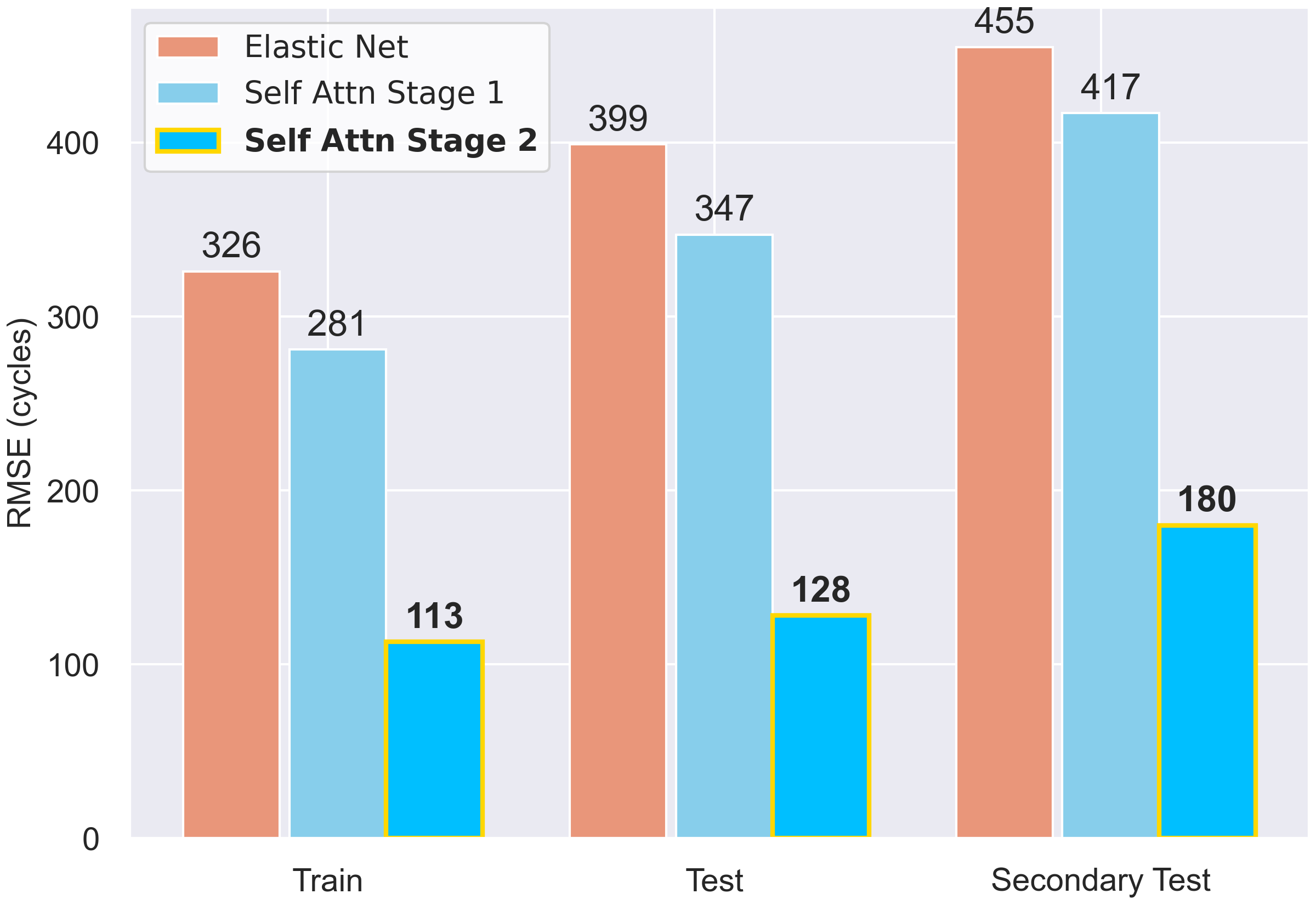
Figure 6: Comparison of RMSE for cycle life predictions made by the elastic net baseline model, the self-attention model after the first stage of training, and the self-attention model after both stages of training.

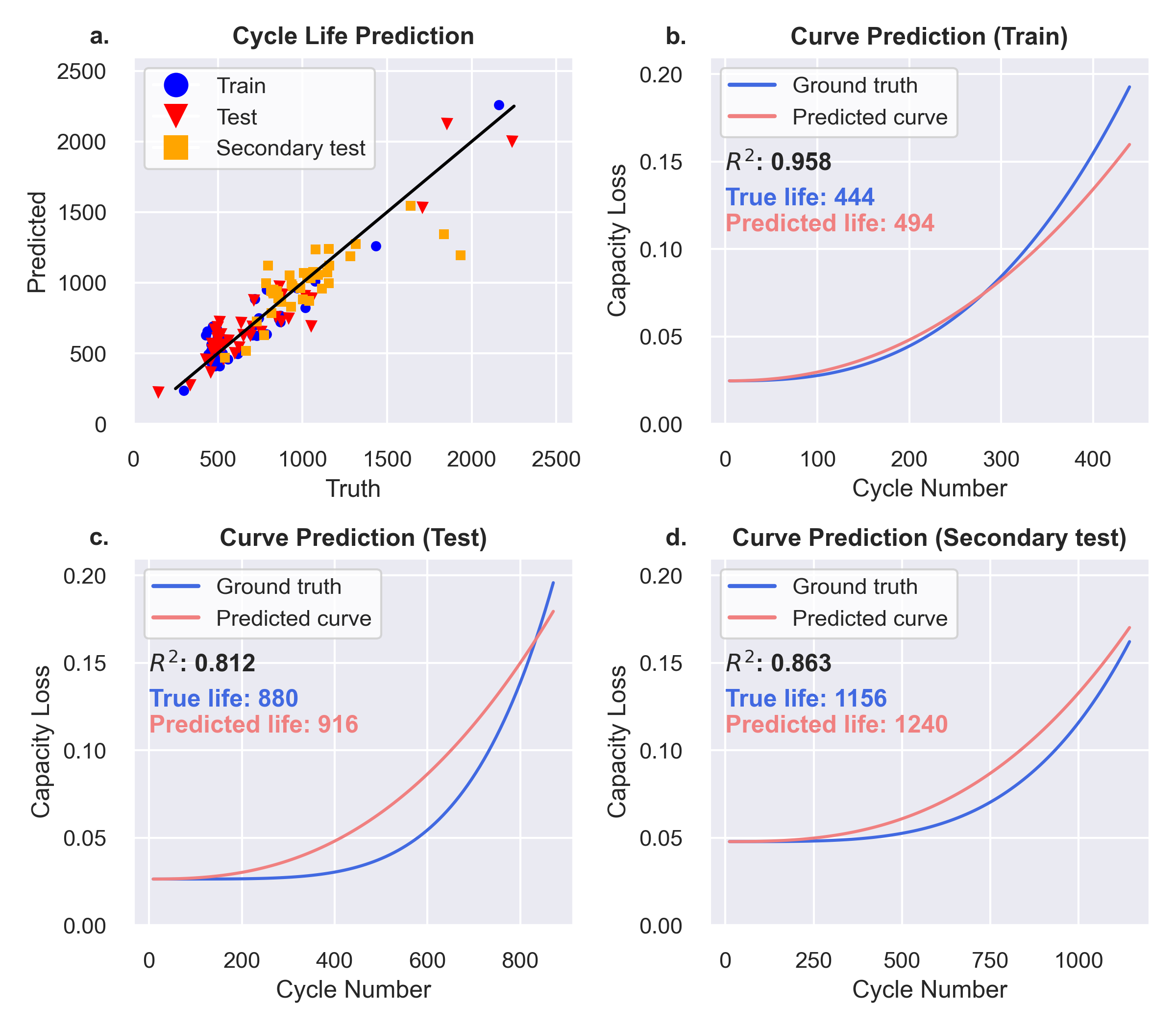
Figure 7: (a) Predicted versus true cycle lives using the self-attention model. (b-d) Predicted versus true capacity curves using the self-attention model for example batteries from the (b) train, (c) test, and (d) secondary test datasets.

5 Conclusion and Future Directions

Our research presents a novel technique of understanding and predicting battery capacity loss curves using a physics-informed model. Our focus on reconstructing these curves rather than on just cycle life prediction offers distinct advantages by providing more robust and interpretable predictions without sacrificing the accuracy achieved in prior work [12]. Parameterizing the ground truth capacity loss curves by fitting an equation inspired from an Arrhenius Law, we train a self-attention model that recovers these parameters and reconstructs the full capacity curves, achieving similar errors to [12]. This approach is flexible to the definition of end of life, offering the advantage of predicting the cycle at which any percent of capacity is lost.

However, there are a few other directions that potentially further improve upon our work. Firstly, we note that battery cycle data is a time series, and hence utilizing entire time series as prediction inputs is one way to incorporate more information and features. This method could potentially improve results given the correct training policy, hyperparameters, and machine learning architectures.

Our method not only provides precise capacity loss forecasts but also incorporates knowledge of the mechanisms underlying battery degradation. The results of this study provide support for the effectiveness of hybrid models, since they combine the best aspects of data-driven and physics-based methodologies. This has the potential to ultimately improve battery life estimation for use in electric vehicles and other socially significant applications.

Data Availability

The datasets used in this paper are available at https://data.matr.io/1.

Code Availability

Data processing and modeling code are available upon request.

Disclosures

C.D Nicolae, S. Sameer, N. Sun, and K. Yan are listed as inventors on a patent application related to this work.

References

- [1] A123 Systems. Battery Pack Design, Validation, and Assembly Guide using A123 Systems Nanophosphate® Cells, 3 2014. Rev. 02.
- [2] M. A. Abu-Seif, A. S. Abdel-Khalik, M. S. Hamad, E. Hamdan, and N. A. Elmalhy. Data-driven modeling for li-ion battery using dynamic mode decomposition. Alexandria Engineering Journal, 61(12):11277–11290, 2022.
- [3] M. Broussely, S. Herreyre, P. Biensan, P. Kasztejna, K. Nechev, and R. Staniewicz. Aging mechanism in li ion cells and calendar life predictions. Journal of Power Sources, 97:13–21, 2001.
- [4] B. Celik, R. Sandt, L. C. P. dos Santos, and R. Spatschek. Prediction of battery cycle life using early-cycle data, machine learning and data management. Batteries, 8(12):266, 2022.
- [5] J. Christensen and J. Newman. A mathematical model for the lithium-ion negative electrode solid electrolyte interphase. Journal of The Electrochemical Society, 151(11):A1977, 2004.
- [6] A. Cordoba-Arenas, S. Onori, Y. Guezennec, and G. Rizzoni. Capacity and power fade cycle-life model for plug-in hybrid electric vehicle lithium-ion battery cells containing blended spinel and layered-oxide positive electrodes. Journal of Power Sources, 278:473–483, 2015.
- [7] T. M. Nguyen, T. M. Nguyen, N. Ho, A. L. Bertozzi, R. Baraniuk, and S. Osher. A primal-dual framework for transformers and neural networks. In The Eleventh International Conference on Learning Representations, 2022.
- [8] B. Pang, L. Chen, and Z. Dong. Data-driven degradation modeling and soh prediction of li-ion batteries. Energies, 15(15):5580, 2022.
- [9] M. B. Pinson and M. Z. Bazant. Theory of sei formation in rechargeable batteries: capacity fade, accelerated aging and lifetime prediction. Journal of the Electrochemical Society, 160(2):A243, 2012.
- [10] A. Rahman and X. Lin. Li-ion battery individual electrode state of charge and degradation monitoring using battery casing through auto curve matching for standard cccv charging profile. Applied Energy, 321:119367, 2022.
- [11] S. Saxena, L. Ward, J. Kubal, W. Lu, S. Babinec, and N. Paulson. A convolutional neural network model for battery capacity fade curve prediction using early life data. Journal of Power Sources, 542:231736, 2022.
- [12] K. A. Severson, P. M. Attia, N. Jin, N. Perkins, B. Jiang, Z. Yang, M. H. Chen, M. Aykol, P. K. Herring, D. Fraggedakis, et al. Data-driven prediction of battery cycle life before capacity degradation. Nature Energy, 4(5):383–391, 2019.
- [13] R. Spotnitz. Simulation of capacity fade in lithium-ion batteries. Journal of Power Sources, 113(1):72–80, 2003.
- [14] C. Strange and G. Dos Reis. Prediction of future capacity and internal resistance of li-ion cells from one cycle of input data. Energy and AI, 5:100097, 2021.
- [15] L. Su, M. Wu, Z. Li, and J. Zhang. Cycle life prediction of lithium-ion batteries based on data-driven methods. ETransportation, 10:100137, 2021.
- [16] A. Vaswani, N. Shazeer, N. Parmar, J. Uszkoreit, L. Jones, A. N. Gomez, Ł. Kaiser, and I. Polosukhin. Attention is all you need. Advances in neural information processing systems, 30, 2017.
- [17] L. von Kolzenberg, A. Latz, and B. Horstmann. Solid–electrolyte interphase during battery cycling: Theory of growth regimes. ChemSusChem, 13(15):3901–3910, 2020.
- [18] J. Wang, P. Liu, J. Hicks-Garner, E. Sherman, S. Soukiazian, M. Verbrugge, H. Tataria, J. Musser, and P. Finamore. Cycle-life model for graphite-lifepo4 cells. Journal of Power Sources, 196(8):3942–3948, 2011.
- [19] R. Wright, J. Christophersen, C. Motloch, J. Belt, C. Ho, V. Battaglia, J. Barnes, T. Duong, and R. Sutula. Power fade and capacity fade resulting from cycle-life testing of advanced technology development program lithium-ion batteries. Journal of Power Sources, 119:865–869, 2003.
- [20] R. B. Wright, C. G. Motloch, J. R. Belt, J. P. Christophersen, C. D. Ho, R. A. Richardson, I. Bloom, S. Jones, V. S. Battaglia, G. Henriksen, et al. Calendar-and cycle-life studies of advanced technology development program generation 1 lithium-ion batteries. Journal of Power Sources, 110(2):445–470, 2002.
- [21] W. W. Xing, A. A. Shah, N. Shah, Y. Wu, Q. Xu, A. Rodchanarowan, P. Leung, X. Zhu, and Q. Liao. Data-driven prediction of li-ion battery degradation using predicted features. Processes, 11(3):678, 2023.
- [22] L. Xu, Z. Deng, Y. Xie, X. Lin, and X. Hu. A novel hybrid physics-based and data-driven approach for degradation trajectory prediction in li-ion batteries. IEEE Transactions on Transportation Electrification, 2022.
- [23] R. Xu, Y. Wang, and Z. Chen. A hybrid approach to predict battery health combined with attention-based transformer and online correction. Journal of Energy Storage, 65:107365, 2023.
- [24] X.-G. Yang, Y. Leng, G. Zhang, S. Ge, and C.-Y. Wang. Modeling of lithium plating induced aging of lithium-ion batteries: Transition from linear to nonlinear aging. Journal of Power Sources, 360:28–40, 2017.
- [25] J. Yao, K. Powell, and T. Gao. A two-stage deep learning framework for early-stage lifetime prediction for lithium-ion batteries with consideration of features from multiple cycles. Frontiers in Energy Research, 10:1059126, 2022.
- [26] J. Zhu, Y. Wang, Y. Huang, R. Bhushan Gopaluni, Y. Cao, M. Heere, M. J. Mühlbauer, L. Mereacre, H. Dai, X. Liu, et al. Data-driven capacity estimation of commercial lithium-ion batteries from voltage relaxation. Nature communications, 13(1):2261, 2022.