S-IQA: IMAGE QUALITY ASSESSMENT WITH COMPRESSIVE SAMPLING

Abstract

No-Reference Image Quality Assessment (IQA) aims at estimating image quality in accordance with subjective human perception. However, most existing NR-IQA methods focus on exploring increasingly complex networks or components to improve the final performance. Such practice imposes great limitations and complexity on IQA methods, especially when they are applied to high-resolution (HR) images in the real world. Actually, most images own high spatial redundancy, especially for those HR data. To further exploit the characteristic and alleviate the issue above, we propose a new framework for Image Quality Assessment with compressive Sampling (dubbed S-IQA), which consists of three components: (1) The Flexible Sampling Module (FSM) samples the image to obtain measurements at an arbitrary ratio. (2) Vision Transformer with the Adaptive Embedding Module (AEM) makes measurements of uniform size and extracts deep features (3) Dual Branch (DB) allocates weight for every patch and predicts the final quality score. Experiments show that our proposed S-IQA achieves state-of-the-art result on various datasets with less data usage.

Index Terms—  Image Quality Assessment, Compressive Sensing, Vision Transformer

1 Introduction

When we access an image from the Internet, it may have passed the following processing stages: captured from a camera, compressed when shared online, spread from people to people, and finally received. Any distortion can be introduced during these stages, which makes our final received image badly degraded from the original one and leaves us annoyed. Low-quality images can also cause deadly problems, especially in autonomous driving. Given these reasons, assessing the quality of images becomes particularly important in our daily lives.

Objective Image Quality Assessment (IQA) employs computational models to provide a quality score of an image from a human’s perspective. Based on the availability of the lossless reference image, objective quality metrics can be divided into full-reference (FR-IQA) and no-reference (NR-IQA) methods. NR-IQA methods are divided mainly into two categories: distortion-based and general-proposed methods. The former aims at predicting quality score towards a certain distortion type, leading to excellent performance but weak generalization. General-proposed methods deal with any kind of distortion but strongly depend on suitable feature extraction. However, as images of high resolution emerge, both methods meet severe computation burden. Actually, instead of the whole image, we might only need a small number of measurements of an image (perhaps 20% measurements) to achieve highly reliable score prediction. In implementation, we employ compressive sensing for sampling.

Compressive sensing (CS) is a novel method that breaks through the limitations of the Nyquist theorem on signal sampling. It demonstrates that a signal can be reconstructed from rather few measurements from the original signal. However, in many applications, such as IQA, the precise reconstructed image isn’t a primary concern. Still, we emphasize more on the final score, which means we can directly perform high-level tasks on the compressed domain, i.e., compressive learning.

The concept of compressive learning (CL) was first proposed by Calderbank et al.[1] and Davenport et al.[2] when they built the inference system directly using measurements without reconstruction. In fact, there are a lot of similarities between measurements and the original image. [3] makes some theoretical works and gradually finds some multidimensional properties of CL. A recent work [4] by Chong Mou et al. employs transformer as the backbone to cope with information loss through element-wise correlations and achieves amazing performance.

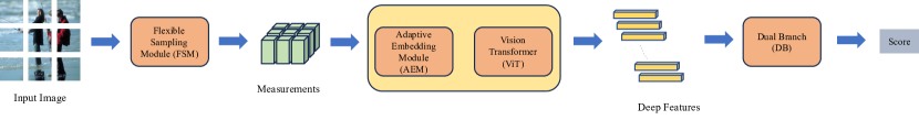
Fig. 1: The architecture of our proposed S-IQA. A distorted image is cropped into non-overlapping 16×16 sized patches. Then the patches are sampled by the FSM to get the compressed measurements. To further extract high-level features, we employ ViT. Moreover, to meet the input shape of transformer, we utilize an Adaptive Embedding Module (AEM) to reshape the measurements. Finally, a dual-branch structure is employed to get the score and weight of each patch and predict the quality score.

Inspired by this work, to make NR-IQA more data-efficient, we propose S-IQA. As shown in Fig.1, S-IQA consists of three parts: A Flexible Sampling Module (FSM), a Vision Transformer with the Adaptive Embedding Module (AEM), and a Dual Branch (DB) for final scoring. The original image is sampled in the flexible sampling module based on the input sampling ratio. Subsequently, the measurements are embedded by an adaptive embedding module and fed into the vision transformer to extract high-level features. Finally, a dual-branch structure is employed for the score prediction.

Our main contributions are as follows: (1) We apply compressive sensing to image quality assessment, enable sampling of images at arbitrary ratios, and achieve amazing performance with a small amount of data. (2) We employ an adaptive embedding module to handle the irregular shape caused by the aforementioned arbitrary sampling ratio. In this way, we can deal with kinds of ratios after training only once. (3) A dual-branch structure is proposed for quality score. In DB, we design scoring and weighting branches for the quality and weight of each patch. We assume that the scores of different parts of the image matter differently, and thus each patch should have its own score and weight.

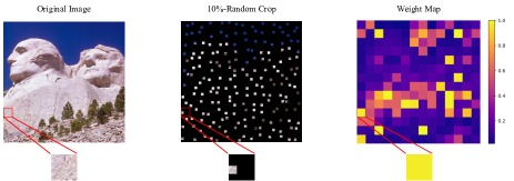
Fig. 2: Random-crop removes pixels from every block despite the importance, leading to severe information loss.

2 RELATED WORK

2.1 Compressive Sensing

Existing CS methods can be classified into two classes: optimization-based and deep-learning-based methods. Traditional optimization-based methods mainly rely on sparsity priors to recover signals from measurements. Some methods attempt to solve it through L1 minimization, such as ISTA, AMP, and BP. There are also data-driven methods that are considered to be more effective than traditional ones, such as [5], [6]. However, the major issue with traditional methods is their extremely high computational complexity due to the iterative calculations. With the development of deep learning, Shi et al.[7] propose a network model called CSNet and show its promising performance. Moreover, some models that mimic traditional methods begin to emerge, such as ISTA-Net and OPINE-Net. Bin Chen et al.[8] use content-aware technique to guide the allocation of sampling ratio and subsequent reconstruction.

2.2 Image Quality Assessment

Unlike FR-IQA, NR-IQA does not have access to reference images. Before the rise of deep learning, traditional methods were mainly divided into natural scene statistics (NSS) metrics and learning-based metrics. The assumption behind this is that the natural scene statistics (NSS) extracted from natural images tend to be highly regular, so distortions to an image would break these statistical regularities and make them detectable. With the success of deep learning and convolution neural networks (CNNs) in computer vision tasks, CNN-based methods have significantly outperformed traditional approaches in handling real-world distortions. Early deep learning NR-IQA methods employed stacked CNNs for feature extraction. [9] proposes a multi-task network where two sub-networks are trained for distortion identification and quality assessment. Hyper-IQA[10] leverages both low-level and high-level features and makes the latter redirect the former. Furthermore, [11] proposes a model that employs meta-learning to capture shared prior knowledge among different distortions.

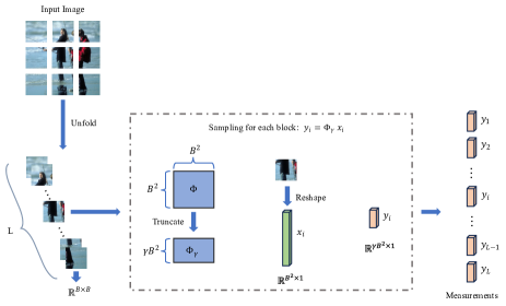
Fig. 3: Process of Flexible Sampling Module (FSM). The input image is split into non-overlapping blocks and then sampled by the same matrix.

3 PROPOSED METHOD

In this section, we elaborate on the details of our framework and integrated model. The whole architecture of our S-IQA is presented in Fig.1, which is mainly composed of a Flexible Sampling Module (FSM), a Vision Transformer with Adaptive Embedding Module (AEM) and a Dual Branch (DB).

Fig. 4: Illustration of Vision Transformer with Adaptive Embedding Module (AEM). The random-shape measurements are embedded into a unified dimension by AEM before fed into ViT for feature extraction.

3.1 Flexible Sampling Module

Among the recent works, there already exist some data-efficient methods for quality assessment, such as FAST-VQA[12] with random-crop. But cropping cannot guarantee that the remained part matters and the removal is almost useless. In Fig.2, we show the original image, 10%-cropped image, and the weight map of the original one. We can observe that even for the block with a large weight, random-crop removes 90% pixels of it. To make full use of the original image and obtain data more reasonably, we introduce compressive sensing.

FSM is employed to compress the image using compressive sensing with sampling matrix $\Phi$, which is learnable. Due to the high computational complexity, previous sampling applications are limited in datasets with low-resolution images like MNIST and CIFAR-10. To extend the model’s applicability to real-world images, we use block-based compressive sensing algorithm (BCS). BCS is able to compress the image block-by-block. As shown in Fig.3, given an image of size $H\times W$ , we split the image into $L=\frac{H}{B}\times\frac{W}{B}$ non-overlapping blocks, with each block sized $B\times B$. To get the measurements, we have a base sampling matrix $\Phi$ sized $B^{2}\times B^{2}$. Noting $\gamma$ as the sampling ratio, we truncate the first $\gamma B^{2}$ rows of $\Phi$ to get $\Phi_{\gamma}$. Finally, to obtain the measurements, the process can be described as follows:

$$y_{i}=\Phi_{\gamma}\cdot x_{i}$$ (1)

where $x_{i}\in\mathbf{R}^{B^{2}}$ represents the flattened block of original image, $y_{i}\in\mathbf{R}^{\gamma B^{2}}$ denotes the corresponding measurement, and $i\in[1,L]$. Throughout the whole process, the only parameter is $\Phi$. To accelerate the computation, we can treat every row of $\Phi_{\gamma}$ as a convolution kernel, which turns matrix multiplication into convolution operation. In each training epoch, by randomly selecting CS ratio, we can get different $\Phi_{\gamma}$ and make it closer to the optimal sampling matrix under ratio $\gamma$. Thus, once trained, we can handle all kinds of arbitrary ratios by only one $\Phi$.

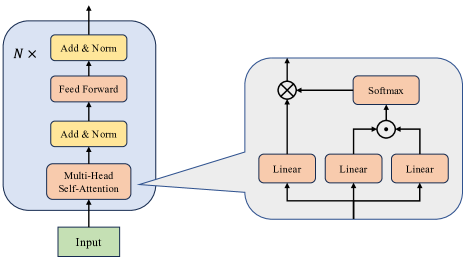
Fig. 5: Flowchart of ViT and multi-head self-attention.

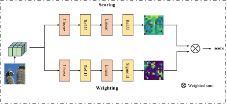
Fig. 6: The dual-branch (DB) structure. Each branch contains two fully connected layers for the score and weight prediction.

Table 1: Comparisons of S-IQA v.s. state-of-the-art NR-IQA algorithms on four standard datasets. The best one is shown in red and the second best in blue.

	LIVE		CSIQ		TID2013		KADID-10K
	PLCC	SRCC	PLCC	SRCC	PLCC	SRCC	PLCC	SRCC
WaDIQaM[13]	0.955	0.960	0.844	0.852	0.855	0.835	0.856	0.851
DBCNN[14]	0.971	0.968	0.959	0.946	0.865	0.816	0.855	0.850
TIQA[15]	0.965	0.949	0.838	0.825	0.858	0.846	0.755	0.762
MetaIQA[11]	0.959	0.960	0.908	0.899	0.868	0.856	0.849	0.840
P2P-BM[16]	0.958	0.959	0.902	0.899	0.856	0.862	0.845	0.852
HyperIQA[10]	0.966	0.962	0.942	0.923	0.858	0.840	0.858	0.915
TReS[17]	0.968	0.969	0.942	0.922	0.883	0.863	0.885	0.872
Re-IQA[18]	0.971	0.970	0.960	0.947	0.861	0.804	0.946	0.944
MANIQA[19]	0.983	0.982	0.968	0.961	0.943	0.937	0.885	0.872
S-IQA-10	0.944	0.936	0.971	0.965	0.930	0.910	0.938	0.933
S-IQA-20	0.975	0.970	0.978	0.970	0.947	0.925	0.942	0.937
S-IQA-50	0.984	0.979	0.983	0.975	0.954	0.944	0.948	0.943

3.2 ViT with Adaptive Embedding Module

Considering that IQA demands a global perception of the whole image, we employ transformer for its excellent performance in constructing long-range correlations. As shown in Fig.4, similar to pure transformer, ViT embeds the input image into the size of $L\times d$, where $d$ denotes the embedding dimension. However, due to the arbitrary CS ratio, the input sequence size $L\times\gamma B^{2}$ is also variable according to the random $\gamma$. To overcome the limitation of the fixed embedding module in ViT, we employ the Adaptive Embedding Module (AEM) to process the measurements. Similar to FSM, we have a base embedding matrix M sized $B^{2}\times B^{2}$. Then, according to the given ratio $\gamma$, we use the first $\gamma B^{2}$ columns of $M$ to form $M_{\gamma}$. Finally, for every measurement $y_{i}$, the embedding process is as follow:

$$t_{i}=M_{\gamma}\cdot y_{i}$$ (2)

Where $t_{i}\in\mathbf{R}^{d}$ represents the sequence that can be handled by ViT. Noting $T=[t_{1},t_{2},…,t_{L}]$ and $P$ as the positional embedding result, the initial input of ViT is constructed by the following formulation:

$$X^{0}=T+P$$ (3)

As illustrated in Fig.5, The standard ViT has the same structure as the transformer encoder, containing a stack of $N$ consecutive blocks. Within each block, the attention mechanism is employed to compute correlations between image patches, finally giving high-level features. The computation process is as follows:

$$\tilde{X}^{i} = Norm(MSA(X^{i-1})+X^{i-1})$$ (4)

$$X^{i} = Norm(FF(\tilde{X}^{i})+\tilde{X}^{i})$$ (5)

Where $MSA$ represents multi-head self-attention, $Norm$ denotes normalization, $FF$ indicates feed forward, $X^{i}$ is the output of the $i$-th block and $i\in[1,N]$.

3.3 Dual Branch

For the final scoring, most of recent IQA methods [10], [11], [17], [18] utilize MLP, i.e., single branch. Nevertheless, when we give a final score of a patch in the image, the clarity is not the only thing of importance, some other factors like aesthetics or the content also matter, which we call weight. To combine the two elements, we design the dual-branch structure for final quality score prediction. As shown in Fig.6, the whole module consists of two independent branches: a scoring branch and a weighting branch. Both branches are rather simple with the same structure except for the last activation function. Given the feature $F=X^{N}$, the final score is obtained by the formula:

$$score=\frac{Sum(S(F)\times W(F))}{Sum(W(F))}$$ (6)

where $S$ indicates scoring branch and $W$ is weighting branch.

4 EXPERIMENTS

4.1 Experimental Settings

We implement our experiments on two NVIDIA GeForce GTX 1080Ti and a computation platform with PyTorch 1.10.0 and CUDA 11.3 version for the whole training, validating, and testing process. We train and evaluate the performance of our proposed model on four datasets: LIVE[20], CSIQ[21], TID2013[22], KADID-10K[23]. Table 2 shows the summary of the datasets that are used in our experiments.

We choose ViT-B/16-224 as our backbone which is pre-trained on ImageNet-21k with patch size set to 16 and image size 224. This base version transformer contains $N$=12 transformer blocks, with the number of heads being 12 in each layer and the dimension of the feature embedding is set to 768. To be consistent with the patch size used in transformer and protect local information correlations, we set the block size in the sampling model also to 16.

Table 2: Summary of IQA datasets.

Dataset	# of DIst. Images	# of Dist Types
LIVE	779	5
CSIQ	866	6
TID2013	3000	24
KADID-10K	10,125	25

In the experiments, we randomly split the dataset into 6:2:2 for training, validating, and testing. During training, we set the batch size to 8. We utilize Adam as the optimizer with learning rate $1\times 10^{-5}$ and weight decay $1\times 10^{-5}$. The training loss we use is Mean Square Error (MSE) loss. During testing, we select the one that performs the best in the validation dataset. For each image in the test dataset, we randomly crop a $224\times 224$ sized patch of it for 5 times and obtain the final score by averaging the results. In our experiments, we evaluate our S-IQA with both fixed CS ratios and arbitrary ratios, and several variants of our model are defined with different names. For instance, “S-IQA-10” represents the variant with a fixed CS ratio of 10%, and “S-IQA-r” denotes the variant that deals with an arbitrary CS ratio.

4.2 Evaluation Criteria

Following the prior works, we employ two commonly used criteria: Spearman’s rank-order correlation coefficient (SRCC) and Pearson’s linear correlation coefficient (PLCC). The SRCC is defined as follows:

$$SRCC=1-\frac{6\sum_{i=1}^{N}(v_{i}-p_{i})}{N(N^{2}-1)}$$ (7)

where $v_{i}$ and $p_{i}$ represent the order of the same image in the ground-truth list and prediction list, and $N$ is the number of images. The PLCC is formulated as:

$$PLCC=\frac{\sum_{i=1}^{N}(y_{i}-\mu_{y_{i}})(\tilde{y}_{i}-\mu_{\tilde{y}_{i}})}{\sqrt{\sum_{i=1}^{N}(y_{i}-\mu_{y_{i}})^{2}}\sqrt{\sum_{i=1}^{N}(\tilde{y}_{i}-\mu_{\tilde{y}_{i}})^{2}}}$$ (8)

where $y_{i}$ and $\tilde{y}_{i}$ indicates the ground-truth and prediction quality score of $i$-th image, and $\mu_{y_{i}}$ and $\mu_{\tilde{y}_{i}}$ denotes the mean of them. Both of the metrics are in [-1, 1]. In our experiments, a higher value means better performance.

Table 3: In the testing stage, ratio-fixed models perform best under the training CS ratio, while S-IQA-r is rather stable.

CS Ratio	PLCC / SRCC
	S-IQA-10	S-IQA-20	S-IQA-50	S-IQA-r
10%	0.971/0.965	0.571/0.550	0.276/0.288	0.962/0.936
20%	0.688/0.629	0.978/0.970	0.772/0.765	0.969/0.953
50%	0.655/0.606	0.822/0.753	0.983/0.975	0.977/0.972
100%	0.751/0.706	0.834/0.780	0.893/0.838	0.976/0.970

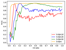
(a) PLCC results.

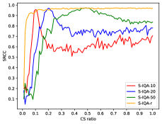
(b) SRCC results.

Fig. 7: PLCC and SRCC of four variants under different CS ratios in CSIQ.

4.3 Comparison with State-of-the-Art Methods

Table 1 shows the overall performance of S-IQA with fixed sampling ratio (10%, 20%, and 50%) on four standard datasets in terms of PLCC and SRCC. We can observe that compared with the methods that utilize the whole image to predict, our proposed S-IQA achieves state-of-the-art performance with much less data. Even if only 10% measurements are available in CSIQ, we can obtain excellent outcomes. Furthermore, one can see that for the same dataset, the performance is getting better with the CS ratio growing, which proves that our sampling module indeed gives more information using a larger CS ratio.

To show the superiority of our FSM, we compare four variants (S-IQA-10/20/50/r) on CSIQ with the CS ratio ranging from 0.01 to 1.0. As shown in Fig.7, except for S-IQA-r, every model with fixed ratio tends to perform better as the CS ratio grows from 0.01. While after the peak, the performance falls fast for the reason that only the first few rows of the sampling matrix are trained (e.g., the first 10% rows of the matrix in S-IQA-10), and as the ratio becomes larger, more and more untrained (i.e., random) parameters participate in calculating and finally destroy the result. In contrast, the whole matrix of FSM in S-IQA-r is trained so it can deal with any ratio once trained. Moreover, the results of S-IQA-r are pretty stable when the CS ratio varies. But Table 3 indicates that despite the flexibility, S-IQA-r cannot beat ratio-fixed variants when the testing ratio exactly equals that of training.

4.4 Visualization

To figure out exactly how the dual-branch structure helps when predicting the quality score, we generate different feature maps using S-IQA-10. As shown in Fig.8, we add White Gaussian Noise to the right half of the image according to different SNRs (10, 1, and 0.1). Similar to what we have assumed, different patches of the image matter differently and the map tends to give more weight to the outline or background. We can observe that with more severe distortion, the score and weight map both give lower values. Among the two, the weight map is dominant and is easier to be affected by noise.

Table 4: Ablation results of ViT and DB at CS ratio=10%.

Module		PLCC / SRCC
ViT	DB	LIVE	CSIQ	TID2013	KADID-10K
2717	2717	0.901/0.890	0.946/0.930	0.897/0.868	0.917/0.911
2713	2717	0.938/0.934	0.966/0.952	0.921/0.897	0.933/0.926
2713	2713	0.944/0.936	0.971/0.965	0.930/0.910	0.938/0.933

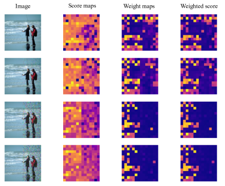
Fig. 8: Dual branch feature maps of an image with different degrees of distortion on the right half. The first row is the pristine image and the SNR from the second row down is 10, 1, and 0.1.

4.5 Ablation Study

In this section, we conduct ablation study on S-IQA-10 to prove the effectiveness of the transformer backbone and the dual branch. For the transformer part, we use ResNet-101 to replace it for feature extraction. In the research of dual branch (DB), we replace it with two layers of CNN and MLP. The result is shown in Table 4. We can observe that each part has a certain effect on the quality prediction. Transformer has the superiority of constructing long-range correlations and the dual-branch can reasonably allocate weight among the patches.

5 CONCLUSION

In this paper, we propose a new data-efficient framework for Image Quality Assessment (IQA) dubbed S-IQA. It first samples the image using the FSM to obtain measurements at any given CS ratio. Then we utilize the AEM to overcome the problem that measurements don’t match the fixed input shape of the transformer. After embedding, the measurements are fed into the Vision Transformer for further feature extraction. Finally, the DB weights every patch of the image and predicts the final quality score. Experimental results demonstrate that with less data usage, our proposed S-IQA outperforms many recent state-of-the-art NR-IQA methods.

References

- [1] Robert Calderbank, Sina Jafarpour, and Robert Schapire, “Compressed learning: Universal sparse dimensionality reduction and learning in the measurement domain,” .
- [2] Mark A. Davenport, Marco F. Duarte, Michael B. Wakin, Jason N. Laska, Dharmpal Takhar, Kevin F. Kelly, and Richard G. Baraniuk, “The smashed filter for compressive classification and target recognition,” in Computational Imaging V, Charles A. Bouman, Eric L. Miller, and Ilya Pollak, Eds. International Society for Optics and Photonics, 2007, vol. 6498, p. 64980H, SPIE.
- [3] Dat Thanh Tran, Mehmet Yamaç, Aysen Degerli, Moncef Gabbouj, and Alexandros Iosifidis, “Multilinear compressive learning,” IEEE Transactions on Neural Networks and Learning Systems, vol. 32, no. 4, pp. 1512–1524, 2021.
- [4] Chong Mou and Jian Zhang, “Transcl: Transformer makes strong and flexible compressive learning,” IEEE Transactions on Pattern Analysis and Machine Intelligence, vol. 45, no. 4, pp. 5236–5251, 2023.
- [5] M. Aharon, M. Elad, and A. Bruckstein, “K-svd: An algorithm for designing overcomplete dictionaries for sparse representation,” IEEE Transactions on Signal Processing, vol. 54, no. 11, pp. 4311–4322, 2006.
- [6] Jian-Feng Cai, Hui Ji, Zuowei Shen, and Gui-Bo Ye, “Data-driven tight frame construction and image denoising,” Applied and Computational Harmonic Analysis, vol. 37, no. 1, pp. 89–105, 2014.
- [7] Wuzhen Shi, Feng Jiang, Shengping Zhang, and Debin Zhao, “Deep networks for compressed image sensing,” in 2017 IEEE International Conference on Multimedia and Expo (ICME), 2017, pp. 877–882.
- [8] Bin Chen and Jian Zhang, “Content-aware scalable deep compressed sensing,” IEEE Transactions on Image Processing, vol. 31, pp. 5412–5426, 2022.
- [9] Kede Ma, Wentao Liu, Kai Zhang, Zhengfang Duanmu, Zhou Wang, and Wangmeng Zuo, “End-to-end blind image quality assessment using deep neural networks,” IEEE Transactions on Image Processing, vol. 27, no. 3, pp. 1202–1213, 2018.
- [10] Shaolin Su, Qingsen Yan, Yu Zhu, Cheng Zhang, Xin Ge, Jinqiu Sun, and Yanning Zhang, “Blindly assess image quality in the wild guided by a self-adaptive hyper network,” in 2020 IEEE/CVF Conference on Computer Vision and Pattern Recognition (CVPR), 2020, pp. 3664–3673.
- [11] Hancheng Zhu, Leida Li, Jinjian Wu, Weisheng Dong, and Guangming Shi, “Metaiqa: Deep meta-learning for no-reference image quality assessment,” in 2020 IEEE/CVF Conference on Computer Vision and Pattern Recognition (CVPR), 2020, pp. 14131–14140.
- [12] Haoning Wu, Chaofeng Chen, Jingwen Hou, Liang Liao, Annan Wang, Wenxiu Sun, Qiong Yan, and Weisi Lin, “Fast-vqa: Efficient end-to-end video quality assessment with fragment sampling,” in European Conference on Computer Vision, 2022.
- [13] Sebastian Bosse, Dominique Maniry, Klaus-Robert Müller, Thomas Wiegand, and Wojciech Samek, “Deep neural networks for no-reference and full-reference image quality assessment,” IEEE Transactions on Image Processing, vol. 27, no. 1, pp. 206–219, 2018.
- [14] Weixia Zhang, Kede Ma, Jia Yan, Dexiang Deng, and Zhou Wang, “Blind image quality assessment using a deep bilinear convolutional neural network,” IEEE Transactions on Circuits and Systems for Video Technology, vol. 30, no. 1, pp. 36–47, 2020.
- [15] Junyong You and Jari Korhonen, “Transformer for image quality assessment,” in 2021 IEEE International Conference on Image Processing (ICIP), 2021, pp. 1389–1393.
- [16] Zhenqiang Ying, Haoran Niu, Praful Gupta, Dhruv Mahajan, Deepti Ghadiyaram, and Alan Bovik, “From patches to pictures (paq-2-piq): Mapping the perceptual space of picture quality,” in 2020 IEEE/CVF Conference on Computer Vision and Pattern Recognition (CVPR), 2020, pp. 3572–3582.
- [17] S. Alireza Golestaneh, Saba Dadsetan, and Kris M. Kitani, “No-reference image quality assessment via transformers, relative ranking, and self-consistency,” in 2022 IEEE/CVF Winter Conference on Applications of Computer Vision (WACV), 2022, pp. 3989–3999.
- [18] Avinab Saha, Sandeep Mishra, and Alan Conrad Bovik, “Re-iqa: Unsupervised learning for image quality assessment in the wild,” 2023 IEEE/CVF Conference on Computer Vision and Pattern Recognition (CVPR), pp. 5846–5855, 2023.
- [19] Sidi Yang, Tianhe Wu, Shu Shi, Shan Gong, Ming Cao, Jiahao Wang, and Yujiu Yang, “Maniqa: Multi-dimension attention network for no-reference image quality assessment,” 2022 IEEE/CVF Conference on Computer Vision and Pattern Recognition Workshops (CVPRW), pp. 1190–1199, 2022.
- [20] H.R. Sheikh, M.F. Sabir, and A.C. Bovik, “A statistical evaluation of recent full reference image quality assessment algorithms,” IEEE Transactions on Image Processing, vol. 15, no. 11, pp. 3440–3451, 2006.
- [21] Eric C. Larson and Damon M. Chandler, “Most apparent distortion: full-reference image quality assessment and the role of strategy,” J. Electronic Imaging, vol. 19, pp. 011006, 2010.
- [22] Nikolay N. Ponomarenko, Lina Jin, Oleg Ieremeiev, Vladimir V. Lukin, Karen, Egiazarian, Jaakko Astola, Benoît Vozel, Kacem Chehdi, Marco Carli, and Federica Battisti, “Image database tid 2013 : Peculiarities , results and perspectives,” 2016.
- [23] Hanhe Lin, Vlad Hosu, and Dietmar Saupe, “Kadid-10k: A large-scale artificially distorted iqa database,” in 2019 Eleventh International Conference on Quality of Multimedia Experience (QoMEX), 2019, pp. 1–3.