Finite volume simulation of a semi-linear
Neumann problem (Keller-Segel model)
on rectangular domains

Abstract

In this study, the finite volume method is implemented for solving the problem of the semi-linear equation: $-d\,\Delta u+u=u^{q}$ ($d,q>0$) with a homogeneous Neumann boundary condition. This problem is equivalent to the known stationary Keller-Segel model, which arises in chemotaxis.After discretization, a nonlinear algebraic system is obtained and solved on the platform Matlab. As a result, many single-peaked and multi-peaked shapes in $3D$ and contour plots can be drawn depending on the parameters $d$ and $q$.

Keywords: Semilinear problem; Neumann condition; Finite volume appraoch; Single-peaked solution; Multipeak solution.

1 Intoduction

In biology, chemotaxis is a type of cell movement that occurs when bodily cells, such as spermatozoa, the tube of pollen grains, bacteria, or other uni- or multicellular organisms, direct themselves or their movements in response to certain chemical species that are present in their environment. It is noteworthy to mention that chemotaxis plays a significant role in the development and physiological functioning of the organism [6, 13].

In 1970, Keller and Segel proposed in [8] a mathematical model in order to represent the process of amoebae transforming into chemotactic aggregates. They introduced a problem for a system of two semi-linear PDEs for the amoeba population $w(x,t)$ and the chemical product concentration $v(x,t)$. This is given as follows:

$$\begin{cases}\;\;\quad\frac{\partial w}{\partial t}=D_{1}\Delta w-\chi\nabla.(w\nabla\phi(v))\qquad x\in\Omega,\;t>0,\\ \;\;\quad\,\frac{\partial v}{\partial t}=D_{2}\Delta v+k(w,v)\qquad\qquad\quad\;x\in\Omega,\;t>0,\\ \;\,\quad\frac{\partial w}{\partial\overrightarrow{n}}=\frac{\partial v}{\partial\overrightarrow{n}}=0\qquad\qquad\qquad\qquad\;\;\;x\in\partial\Omega,\;t>0,\\ w(x,0)=w_{0}(x)>0\qquad\qquad\qquad\quad\;\;\,x\in\Omega,\\ \;v(x,0)=v_{0}(x)>0\qquad\qquad\qquad\qquad x\in\Omega,\end{cases}$$ (1)

where $\Omega$ is a bounded domain in $\mathbb{R}^{N}$ with a regular boundary $\partial\Omega$, $\phi$ a real function such as $\phi^{{}^{\prime}}(r)>0$ for any $r>0$, $k(w,v)$ a real function with $k_{w}\geq 0$, $k_{v}\leq 0$ and $\overrightarrow{n}$ denotes the unit outer normal to $\partial\Omega$, whereas $D_{1}$, $D_{2}$ and $\chi$ are positive given constants. Here, as usual,

$$\Delta={\sum_{i=1}^{N}}\frac{\partial^{2}}{\partial x_{i}^{2}},\quad\nabla=\left[\frac{\partial}{\partial x_{1}}\;\frac{\partial}{\partial x_{2}}\;\ldots\;\frac{\partial}{\partial x_{N}}\right]^{T}.$$

A simple functional transformation reduces problem (1) in its stationary version to the equivalent problem for a single semi-linear PDE (see [11]):

$$\left\{\begin{array}[]{c}-d\,\Delta u+u=u^{q}\ \ \ \ \text{in }\Omega\\ \frac{\partial u}{\partial\overrightarrow{n}}=0\ \ \ \ \ \ \ \ \ \ \ \ \ \ \ \ sur\text{ }\partial\Omega\\ u>0\text{ \ \ \ \ \ \ \ \ \ \ \ \ \ \ \ \ \ }\text{ for}\Omega\end{array}\right.$$ (2)

with $d$ and $q$ being given positive constants. This problem arises in the investigation of steady-state solutions to certain reaction-diffusion systems involved in chemotaxis and morphogenesis. Therefore, it is widely studied to ensure the best understanding of this phenomenon. The existence and uniqueness of the least-energy solution to the problem (2) have been proven in the literature (see, e.g., [4, 9, 11]). However, many studies are focusing on the shape of the solution. In this respect, single-peaked and multi-peaked solutions are theoretically found in [1, 2, 15, 18] and predicting their locations [16]. In addition, the boundary spike layer solutions are obtained and studied in [10, 17, 19]. A numerical study based on the fast Fourier solver has been applied in [7] to the problem (2) in order to investigate various solution forms.

The finite volume method is a well-adapted discretization technique for various types of simulation of conservation laws in elliptic, parabolic, hyperbolic, and other PDE situations like in [3, 5, 14]. During the last two decades, it has been applied in several engineering branches such as fluid mechanics, heat and mass transfer, and petroleum engineering. In the present work, the finite volume technique is applied to the problem (2) on a bi-dimensional domain. As a consequence, a nonlinear system is obtained and directly solved on Matlab to produce single-peaked and multi-peaked discrete solutions.

2 Application of the finite volume method

Consider the problem (2) on the rectangular domain $\Omega=\left]L_{x_{1}},L_{x_{2}}\right[\times\left]L_{y_{1}},L_{y_{2}}\right[$. In addition, the boundary is set as $\partial\Omega=\Gamma_{1}\cup\Gamma_{2}\cup\Gamma_{3}\cup\Gamma_{4}$, with:

$$\Gamma_{1}=\left[L_{x_{1}},L_{x2}\right]\times\left\{L_{y_{1}}\right\},\quad\Gamma_{2}=\left\{L_{x_{1}}\right\}\times\left[L_{y_{1}},L_{y_{2}}\right],\quad\Gamma_{3}=\left\{L_{x_{2}}\right\}\times\left[L_{y_{1}},L_{y}\right],\quad\Gamma_{4}=\left[L_{x_{1}},L_{x_{2}}\right]\times\left\{L_{y_{2}}\right\}.$$ (3)

$\Omega$ is partitioned into $N\times P$ control volumes $\Omega_{i,j}$ with center points $(x_{i},y_{j})$ ($i=1,\ldots,N$ and $j=1,\ldots,P$). By choosing the midpoints: $x_{i+1/2}=\dfrac{x_{i}+x_{i+1}}{2}$, $y_{i+1/2}=\dfrac{y_{i}+y_{i+1}}{2}$, set: $h_{x}=x_{i+1/2}-x_{i-1/2}$ and $h_{y}=y_{j+1/2}-y_{j-1/2}$ as the steps.
Therefore,

$$\Omega_{i,j}=\left]x_{i-\frac{1}{2}},x_{i+\frac{1}{2}}\right[\times\left]y_{j-\frac{1}{2}},y_{j+\frac{1}{2}}\right[.$$ (4)

The boundary of each control volume $\Omega_{i,j}$ is denoted by $\partial\Omega_{i,j}$ with $\partial\Omega_{i,j}=\bigcup_{i=1}^{k}\Gamma_{k}^{i,j}$, and we set:

$$\Gamma_{1}^{i,j}=\left[x_{i-\frac{1}{2}},x_{i+\frac{1}{2}}\right]\times\left\{y_{j-\frac{1}{2}}\right\},\quad\Gamma_{2}^{i,j}=\left\{x_{i-\frac{1}{2}}\right\}\times\left[y_{j-\frac{1}{2}},y_{j+\frac{1}{2}}\right],$$

$$\Gamma_{3}^{i,j}=\left\{x_{i+\frac{1}{2}}\right\}\times\left[y_{j-\frac{1}{2}},y_{j+\frac{1}{2}}\right],\quad\Gamma_{4}^{i,j}=\left[x_{i-\frac{1}{2}},x_{i+\frac{1}{2}}\right]\times\left\{y_{j+\frac{1}{2}}\right\}.$$ (5)

A representative control volume $\Omega_{i,j}$ of the domain discretization is illustrated in Figure 1.

The discrete solution is assumed to be constant in each control volume $\Omega_{i,j}$ and equal to an approximate value $u_{ij}$ of the average $u(x_{i},y_{j})$ in the control volume $\Omega_{i,j}$.

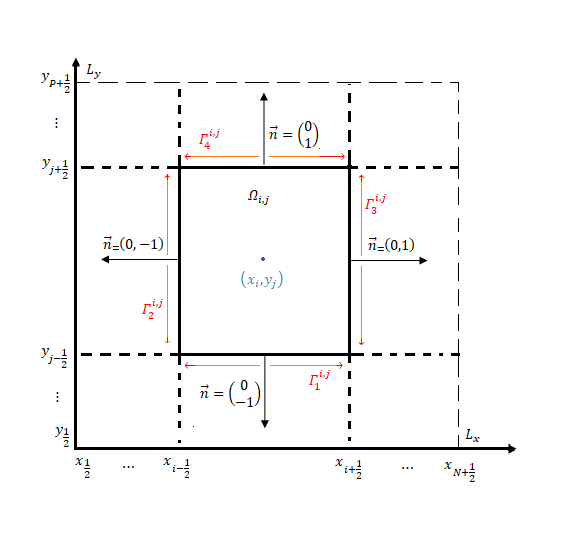
Figure 1: The control volume $\Omega_{i,j}$ in the domain $\Omega$.

Finite volume discretization starts from integrating the PDE of the problem (2) on each control volume. In so doing, we get

$$-d\int_{\Omega_{i,j}}\Delta u(x,y)\text{ }dxdy+\int_{\Omega_{i,j}}u(x,y)\text{ }dxdy=\int_{\Omega_{i,j}}\left[u(x,y)\right]^{q}dxdy,$$ (6)

so that the divergence formula yields

$$-d\int_{\partial\Omega_{i,j}}\nabla u\cdot\overrightarrow{n}\text{ }ds+h_{x}h_{y}u_{i,j}=h_{x}h_{y}\left(u_{i,j}\right)^{q}.$$ (7)

Therefore, we obtain

$$\small-d\int_{\Gamma_{1}^{i,j}}\nabla u\cdot\overrightarrow{n}\text{ }ds-d\int_{\Gamma_{2}^{i,j}}\nabla u\cdot\overrightarrow{n}\text{ }ds-d\int_{\Gamma_{3}^{i,j}}\nabla u\cdot\overrightarrow{n}\text{ }ds-d\int_{\Gamma_{4}^{i,j}}\nabla u\cdot\overrightarrow{n}\text{ }ds+h_{x}h_{y}u_{i,j}=h_{x}h_{y}\left(u_{i,j}\right)^{q}.$$ (8)

Now, let us proceed to fluxes calculation $\int_{\Gamma_{k}^{i,j}}\nabla u.\overrightarrow{n}$ $ds$ for $k=1,2,3,4$. For $k=1$, we have $\overrightarrow{n}=\dbinom{0}{-1}$, so that:

$$\int_{\Gamma_{1}^{i,j}}\nabla u\cdot\overrightarrow{n}\text{ }ds= -\int_{\Gamma_{1}^{i,j}}\frac{\partial u}{\partial y}\text{ \ }ds\text{ }$$ (9)

$$= -\int_{x_{i-\frac{1}{2}}}^{x_{i+\frac{1}{2}}}\frac{\partial u}{\partial y}\left(x,y_{j-\frac{1}{2}}\right)\text{\ }dx.$$

By selecting the average value of $\frac{\partial u}{\partial y}\left(x,y_{j-\frac{1}{2}}\right)$ on the segment $\left[x_{i-\frac{1}{2}},x_{i+\frac{1}{2}}\right]$ as being $\frac{\partial u}{\partial y}\left(x_{i},y_{j-\frac{1}{2}}\right)$, we can find:

$$\int_{\Gamma_{1}^{i,j}}\nabla u\cdot\overrightarrow{n}\text{ }ds=-h_{x}\frac{\partial u}{\partial y}\left(x_{i},y_{j-\frac{1}{2}}\right).$$ (10)

On the other hand, an approximation of $\frac{\partial u}{\partial y}\left(x_{i},y_{j-\frac{1}{2}}\right)$ can be given by:

$$\frac{\partial u}{\partial y}\left(x_{i},y_{j-\frac{1}{2}}\right)\cong\frac{u_{i,j}-u_{i,j-1}}{h_{y}}.$$ (11)

Hence,

$$\int_{\Gamma_{1}^{i,j}}\nabla u\cdot\overrightarrow{n}ds=\frac{h_{x}}{h_{y}}\left(u_{i,j-1}-u_{i,j}\right).$$ (12)

Similar steps can be repeated for evaluating the other integrals in (8). We successively get:

for $k=2$ with $\overrightarrow{n}=\dbinom{-1}{0}$:

$$\int_{\Gamma_{2}^{i,j}}\nabla u.\overrightarrow{n}\text{ }ds=\frac{h_{y}}{h_{x}}(u_{i-1,j}-u_{i,j}),$$ (13)

for $k=3$ with $\overrightarrow{n}=\dbinom{1}{0}$:

$$\int_{\Gamma_{3}^{i,j}}\nabla u.\overrightarrow{n}ds=\frac{h_{y}}{h_{x}}(u_{i+1,j}-u_{i,j}),$$ (14)

for $k=4$ with $\overrightarrow{n}=\dbinom{0}{1}$:

$$\int_{\Gamma_{4}^{i,j}}\nabla u.\overrightarrow{n}ds=\frac{h_{x}}{h_{y}}\left(u_{i,j+1}-u_{i,j}\right).$$ (15)

The substitution of (12)-(15) into (8) yields for all $i=1,\ldots,N$ et $j=1,\ldots,P$:

$$-d\left[\frac{h_{x}}{h_{y}}\left(u_{i,j-1}-u_{i,j}\right)+\frac{h_{y}}{h_{x}}\left(u_{i-1,j}-u_{i,j}\right)+\frac{h_{y}}{h_{x}}\left(u_{i+1,j}-u_{i,j}\right)+\frac{h_{x}}{h_{y}}\left(u_{i,j+1}-u_{i,j}\right)\right]+h_{x}h_{y}\left[u_{i,j}-\left(u_{i,j}\right)^{q}\right]=0.$$ (16)

Next, depending on the control volume $\Omega_{i,j}$, this equation takes different forms because boundary processing requires special attention. First, it is important to note that this equation is valid for any control volume whose boundary does not meet $\partial\Omega$. This concerns control volumes $\Omega_{i,j}$ with $i=2,\ldots,N-1$ and $j=2,\ldots,P-1$. For instance, equation (16) can display a new form for the control volume $\Omega_{1,1}$ using the boundary condition. Therefore, as the Neumann condition is homogeneous on the boundary, it follows that $\int_{\Gamma_{1}^{1,1}}\nabla u\cdot\overrightarrow{n}\,ds=\int_{\Gamma_{2}^{1,1}}\nabla u\cdot\overrightarrow{n}\,=0$, as $u_{1,0}=u_{1,1}$ and $u_{0,1}=u_{1,1}$. In this case, equation (16) can be rewritten in the form:

$$-d\left[\frac{h_{y}}{h_{x}}\left(u_{2,1}-u_{1,1}\right)+\frac{h_{x}}{h_{y}}\left(u_{1,2}-u_{1,1}\right)\right]+h_{x}h_{y}\left[u_{1,1}-\left(u_{1,1}\right)^{q}\right]=0\text{ }$$ (17)

Following the same calculation path, we can obtain the corresponding equation for each control volume neighboring the boundary of the domain. Finally, the discretization by finite volumes is summarized by the following system of nonlinear equations:

$$\left\{\begin{array}[]{c}{\small j=1}\text{ \ \ \ \ \ \ \ \ \ \ \ \ \ \ \ \ \ \ \ \ \ \ \ \ \ \ \ \ \ \ \ \ \ \ \ \ \ \ \ \ \ \ \ \ \ \ \ \ \ \ \ \ \ \ \ \ \ \ \ \ \ \ \ \ \ \ \ \ \ \ \ \ \ \ \ \ \ \ \ \ \ \ \ \ \ \ }\\ \left\{\begin{array}[]{c}{\small i=1}\text{ \ \ \ \ \ \ \ \ \ \ \ \ \ \ \ \ \ \ \ \ \ \ \ \ \ \ \ \ \ \ \ \ \ \ \ \ \ \ \ \ \ \ \ \ \ \ \ \ \ \ \ \ \ \ \ \ \ \ \ \ \ \ \ \ \ \ \ \ \ \ \ \ \ \ \ \ \ \ \ \ \ \ \ \ \ \ \ \ \ }\\ \left[h_{x}h_{y}+d\left(\frac{h_{x}}{h_{y}}+\frac{h_{y}}{h_{x}}\right)\right]{\small u}_{1,1}{\small-d}\frac{h_{y}}{h_{x}}{\small u}_{2,1}{\small-d}\frac{h_{x}}{h_{y}}{\small u}_{1,2}{\small-h}_{x}{\small h}_{y}\left(u_{1,1}\right)^{q}{\small=0}\text{ \ \ \ \ \ \ \ \ \ \ \ \ \ \ \ \ \ \ \ \ \ \ \ \ \ \ \ \ \ \ \ \ \ \ \ \ \ \ \ \ \ \ \ \ \ \ \ \ \ \ \ \ \ \ \ \ \ \ \ \ \ \ \ \ \ \ \ \ \ \ \ \ \ \ \ \ \ \ \ \ \ \ \ \ \ \ \ \ \ \ }\\ {\small i=}\overline{\text{\ }2,N-1}\text{ \ \ \ \ \ \ \ \ \ \ \ \ \ \ \ \ \ \ \ \ \ \ \ \ \ \ \ \ \ \ \ \ \ \ \ \ \ \ \ \ \ \ \ \ \ \ \ \ \ \ \ \ \ \ \ \ \ \ \ \ \ \ \ \ \ \ \ \ \ \ \ \ \ \ \ \ \ \ \ \ \ \ \ \ \ \ \ }\\ {\small-d}\frac{h_{y}}{h_{x}}{\small u}_{i-1,1}{\small+}\left[h_{x}h_{y}+d\left(\frac{h_{x}}{h_{y}}+2\frac{h_{y}}{h_{x}}\right)\right]{\small u}_{i,1}{\small-d}\frac{h_{y}}{h_{x}}{\small u}_{i+1,1}{\small-d}\frac{h_{x}}{h_{y}}{\small u}_{i,2}{\small-h}_{x}{\small h}_{y}\left(u_{i,1}\right)^{q}{\small=0}\text{ \ \ \ \ \ \ \ \ \ \ \ \ \ \ \ \ \ \ \ \ \ \ \ \ \ \ \ \ \ \ \ \ \ \ \ \ \ \ \ \ \ \ \ \ \ \ \ \ \ \ \ \ \ \ \ \ \ \ \ \ \ \ \ \ \ \ \ \ \ \ \ \ \ \ }\\ {\small i=N}\text{\ \ \ \ \ \ \ \ \ \ \ \ \ \ \ \ \ \ \ \ \ \ \ \ \ \ \ \ \ \ \ \ \ \ \ \ \ \ \ \ \ \ \ \ \ \ \ \ \ \ \ \ \ \ \ \ \ \ \ \ \ \ \ \ \ \ \ \ \ \ \ \ \ \ \ \ \ \ \ \ \ \ \ \ \ \ \ \ \ }\\ {\small-d}\frac{h_{y}}{h_{x}}{\small u}_{N-1,1}{\small+}\left[h_{x}h_{y}+d\left(\frac{h_{x}}{h_{y}}+\frac{h_{y}}{h_{x}}\right)\right]{\small u}_{N,1}{\small-d}\frac{h_{x}}{h_{y}}{\small u}_{N,2}{\small-h}_{x}{\small h}_{y}\left(u_{N,1}\right)^{q}{\small=0}\text{ \ \ \ \ \ \ \ \ \ \ \ \ \ \ \ \ \ \ \ \ \ \ \ \ \ \ \ \ \ \ \ \ \ \ \ \ \ \ \ \ \ \ \ \ \ \ \ \ \ \ \ \ \ \ \ \ \ \ \ \ \ \ \ \ \ \ \ \ \ \ \ \ \ \ \ \ \ \ \ \ \ \ \ \ \ }\end{array}\right.\\ {\small j=}\overline{2,P-1}\text{ \ \ \ \ \ \ \ \ \ \ \ \ \ \ \ \ \ \ \ \ \ \ \ \ \ \ \ \ \ \ \ \ \ \ \ \ \ \ \ \ \ \ \ \ \ \ \ \ \ \ \ \ \ \ \ \ \ \ \ \ \ \ \ \ \ \ \ \ \ \ \ \ \ \ \ \ \ \ \ \ \ \ \ }\\ \left\{\begin{array}[]{c}{\small i=1}\text{\ \ \ \ \ \ \ \ \ \ \ \ \ \ \ \ \ \ \ \ \ \ \ \ \ \ \ \ \ \ \ \ \ \ \ \ \ \ \ \ \ \ \ \ \ \ \ \ \ \ \ \ \ \ \ \ \ \ \ \ \ \ \ \ \ \ \ \ \ \ \ \ \ \ \ \ \ \ \ \ \ \ \ \ \ \ \ \ \ }\\ {\small-d}\frac{h_{x}}{h_{y}}{\small u}_{1,j-1}{\small+}\left[h_{x}h_{y}+d\left(2\frac{h_{x}}{h_{y}}+\frac{h_{y}}{h_{x}}\right)\right]{\small u}_{1,j}{\small-d}\frac{h_{y}}{h_{x}}{\small u}_{2,j}{\small-d}\frac{h_{x}}{h_{y}}{\small u}_{1,j+1}{\small-h}_{x}{\small h}_{y}\left(u_{1,j}\right)^{q}{\small=0}\text{ \ \ \ \ \ \ \ \ \ \ \ \ \ \ \ \ \ \ \ \ \ \ \ \ \ \ \ \ \ \ \ \ \ \ \ \ \ \ \ \ \ \ \ \ \ \ \ \ \ \ \ \ \ \ \ \ \ \ \ \ \ \ \ \ \ \ \ \ \ \ }\\ {\small i=}\overline{\text{\ }2,N-1}\text{ \ \ \ \ \ \ \ \ \ \ \ \ \ \ \ \ \ \ \ \ \ \ \ \ \ \ \ \ \ \ \ \ \ \ \ \ \ \ \ \ \ \ \ \ \ \ \ \ \ \ \ \ \ \ \ \ \ \ \ \ \ \ \ \ \ \ \ \ \ \ \ \ \ \ \ \ \ \ \ \ \ \ \ \ \ \ \ }\\ {\small-d}\frac{h_{x}}{h_{y}}{\small u}_{i,j-1}{\small-d}\frac{h_{y}}{h_{x}}{\small u}_{i-1,j}{\small+}\left[h_{x}h_{y}+2d\left(\frac{h_{x}}{h_{y}}+\frac{h_{y}}{h_{x}}\right)\right]{\small u}_{i,j}{\small-d}\frac{h_{y}}{h_{x}}{\small u}_{i+1,j}-\text{ \ \ \ \ \ \ \ \ \ \ \ \ \ \ \ \ \ \ \ \ \ \ \ \ \ \ \ \ \ \ \ \ \ \ \ \ \ \ \ \ \ \ \ \ \ \ \ \ \ \ \ \ \ \ \ \ \ \ \ \ \ \ \ \ \ \ \ \ \ \ \ \ \ \ \ \ \ \ \ \ \ \ \ \ \ \ \ \ \ }\\ {\small d}\frac{h_{x}}{h_{y}}{\small u}_{i,j+1}{\small-h}_{x}{\small h}_{y}\left(u_{i,j}\right)^{q}{\small=0}\text{\ \ \ \ \ \ \ \ \ \ }\\ {\small i=N}\text{ \ \ \ \ \ \ \ \ \ \ \ \ \ \ \ \ \ \ \ \ \ \ \ \ \ \ \ \ \ \ \ \ \ \ \ \ \ \ \ \ \ \ \ \ \ \ \ \ \ \ \ \ \ \ \ \ \ \ \ \ \ \ \ \ \ \ \ \ \ \ \ \ \ \ \ \ \ \ \ \ }\\ {\small-d}\frac{h_{x}}{h_{y}}{\small u}_{N,j-1}{\small-d}\frac{h_{y}}{h_{x}}{\small u}_{N-1,j}{\small+}\left[h_{x}h_{y}+d\left(2\frac{h_{x}}{h_{y}}+\frac{h_{y}}{h_{x}}\right)\right]{\small u}_{N,j}{\small-d}\frac{h_{x}}{h_{y}}{\small u}_{N,j+1}{\small-}\text{ \ \ \ \ \ \ \ \ \ \ \ \ \ \ \ \ \ \ \ \ \ \ \ \ \ \ \ \ \ \ \ \ \ \ \ \ \ \ \ \ \ \ \ \ \ \ \ \ \ \ \ \ \ \ \ \ \ \ \ \ \ \ \ \ \ \ \ \ \ \ \ \ \ \ \ \ \ \ \ \ \ \ \ \ \ \ \ \ }\\ \text{ \ \ \ \ \ \ \ \ \ \ \ \ \ \ \ \ \ \ \ \ \ \ \ \ \ \ \ \ \ \ \ \ \ \ \ \ \ \ \ \ \ \ \ \ \ \ \ \ \ \ \ \ \ \ \ \ \ \ \ \ \ \ \ \ \ \ \ \ \ \ \ \ \ \ \ \ \ \ }{\small h}_{x}{\small h}_{y}\left(u_{N,j}\right)^{q}{\small=0}\text{ \ \ \ \ \ \ \ \ \ \ \ \ \ \ \ \ \ \ \ \ \ \ \ \ \ \ \ \ \ \ \ \ \ \ \ \ \ \ \ \ \ \ \ \ \ \ \ \ \ \ \ \ \ \ \ \ \ \ \ \ \ \ \ \ \ \ \ \ \ \ \ \ \ }\\ \text{\ \ \ \ \ \ \ \ }\end{array}\right.\\ {\small j=P}\text{ \ \ \ \ \ \ \ \ \ \ \ \ \ \ \ \ \ \ \ \ \ \ \ \ \ \ \ \ \ \ \ \ \ \ \ \ \ \ \ \ \ \ \ \ \ \ \ \ \ \ \ \ \ \ \ \ \ \ \ \ \ \ \ \ \ \ \ \ \ \ \ \ \ \ }\\ \left\{\begin{array}[]{c}{\small i=1}\text{ \ \ \ \ \ \ \ \ \ \ \ \ \ \ \ \ \ \ \ \ \ \ \ \ \ \ \ \ \ \ \ \ \ \ \ \ \ \ \ \ \ \ \ \ \ \ \ \ \ \ \ \ \ \ \ \ \ \ \ \ \ \ \ \ \ \ \ \ \ \ \ \ \ \ \ \ \ \ }\\ {\small-d}\frac{h_{x}}{h_{y}}{\small u}_{1,P-1}{\small+}\left[h_{x}h_{y}+d\left(\frac{h_{x}}{h_{y}}+\frac{h_{y}}{h_{x}}\right)\right]{\small u}_{1,P}{\small-d}\frac{h_{y}}{h_{x}}{\small u}_{2,P}{\small-h}_{x}{\small h}_{y}\left(u_{1,P}\right)^{q}{\small=0}\text{ \ \ \ \ \ \ \ \ \ \ \ \ \ \ \ \ \ \ \ \ \ \ \ \ \ \ \ \ \ \ \ \ \ \ \ \ \ \ \ \ \ \ \ \ \ \ \ \ \ \ \ \ \ \ \ \ \ \ \ \ \ \ \ \ \ \ \ \ \ \ \ \ \ \ \ \ \ \ \ \ \ \ \ \ \ }\\ {\small i=}\overline{\text{\ }2,N-1}\text{\ \ \ \ \ \ \ \ \ \ \ \ \ \ \ \ \ \ \ \ \ \ \ \ \ \ \ \ \ \ \ \ \ \ \ \ \ \ \ \ \ \ \ \ \ \ \ \ \ \ \ \ \ \ \ \ \ \ \ \ \ \ \ \ \ \ \ \ \ \ \ \ \ \ \ \ \ }\\ {\small-d}\frac{h_{x}}{h_{y}}{\small u}_{i,P-1}{\small-d}\frac{h_{y}}{h_{x}}{\small u}_{i-1,P}{\small+}\left[h_{x}h_{y}+d\left(2\frac{h_{y}}{h_{x}}+\frac{h_{x}}{h_{y}}\right)\right]{\small u}_{i,p}{\small-d}\frac{h_{y}}{h_{x}}{\small u}_{i+1,P}{\small-}\text{ \ \ \ \ \ \ \ \ \ \ \ \ \ \ \ \ \ \ \ \ \ \ \ \ \ \ \ \ \ \ \ \ \ \ \ \ \ \ \ \ \ \ \ \ \ \ \ \ \ \ \ \ \ \ \ \ \ \ \ \ \ \ \ \ \ \ \ \ \ \ \ \ \ \ \ \ \ \ \ \ \ \ \ \ \ \ \ \ \ }\\ {\small h}_{x}{\small h}_{y}\left(u_{i,P}\right)^{q}=0\text{\ \ \ \ }\\ {\small i=N}\text{ \ \ \ \ \ \ \ \ \ \ \ \ \ \ \ \ \ \ \ \ \ \ \ \ \ \ \ \ \ \ \ \ \ \ \ \ \ \ \ \ \ \ \ \ \ \ \ \ \ \ \ \ \ \ \ \ \ \ \ \ \ \ \ \ \ \ \ \ \ \ \ \ \ \ \ \ \ }\\ {\small-d}\frac{h_{x}}{h_{y}}{\small u}_{N,P-1}{\small-d}\frac{h_{y}}{h_{x}}{\small u}_{N-1,P}{\small+}\left[h_{x}h_{y}+d\left(\frac{h_{y}}{h_{x}}+\frac{h_{x}}{h_{y}}\right)\right]{\small u}_{N,p}{\small-h}_{x}{\small h}_{y}\left(u_{N,P}\right)^{q}{\small=0}\text{ \ \ \ \ \ \ \ \ \ \ \ \ \ \ \ \ \ \ \ \ \ \ \ \ \ \ \ \ \ \ \ \ \ \ \ \ \ \ \ \ \ \ \ \ \ \ \ \ \ \ \ \ \ \ \ \ \ \ \ \ \ \ \ \ \ \ \ \ \ \ \ \ \ \ \ \ \ \ \ \ \ }\end{array}\right.\end{array}\right.$$ (18)

3 Numerical test

In this section, we assume that $L_{x_{1}}=L{y_{1}}$ and $L_{x_{2}}=L_{y_{2}}$ and we suppose a uniform mesh by setting: $h_{x}=h_{y}=h$. As a consequence, we get $N=P$. Introducing a new notation of $u_{i,j}$ (for $i=\overline{1,N}$ and $j=\overline{1,N}$) of the system (2) by $X_{S}$ (for $S=\overline{1,N^{2}}$) such that single-index numbering is performed conventionally from left to right and from bottom to top. We also take $s=(j-1)N+i$ for $j=\overline{1,N}$ and $i=\overline{1,N}$ as in Figure 2.

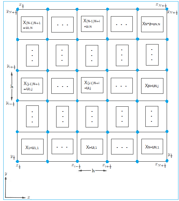
Figure 2: Notation illustration.

For the sake of simplification, we set $a=h^{2}+2d$, $b=h^{2}+3d$, and $c=h^{2}+4d$ in the system (18) to get the following equivalent nonlinear system:

$$\left\{\begin{array}[]{c}j=1\text{ \ \ \ \ \ \ \ \ \ \ \ \ \ \ \ \ \ \ \ \ \ \ \ \ \ \ \ \ \ \ \ \ \ \ \ \ \ \ \ \ \ \ \ \ \ \ \ \ \ \ \ \ \ \ \ \ \ \ \ \ \ \ \ \ \ \ \ \ \ \ }\\ \left\{\begin{array}[]{c}i=1\text{ \ \ \ \ \ \ \ \ \ \ \ \ \ \ \ \ \ \ \ \ \ \ \ \ \ \ \ \ \ \ \ \ \ \ \ \ \ \ \ \ \ \ \ \ \ \ \ \ \ \ \ \ \ \ \ \ \ \ \ \ \ \ \ \ \ \ \ \ \ \ \ \ \ }\\ \left(a-h^{2}X_{1}^{q-1}\right)X_{1}-dX_{2}-dX_{N+1}=0,\text{ \ \ \ \ \ \ \ \ \ \ \ \ \ \ \ \ \ \ \ \ \ \ \ \ \ \ \ \ \ \ \ \ \ \ \ \ \ \ \ \ \ \ \ \ \ \ \ \ \ \ \ \ \ \ \ \ \ \ \ \ \ \ \ \ \ \ \ \ \ \ \ \ \ \ \ \ \ \ \ \ \ \ \ \ \ \ \ \ \ \ \ \ \ \ \ \ \ \ \ \ \ \ \ \ \ \ }\\ i=\overline{2,N-1}\text{ \ \ \ \ \ \ \ \ \ \ \ \ \ \ \ \ \ \ \ \ \ \ \ \ \ \ \ \ \ \ \ \ \ \ \ \ \ \ \ \ \ \ \ \ \ \ \ \ \ \ \ \ \ \ \ \ \ \ \ \ \ \ \ \ \ \ \ \ \ \ \ \ }\\ -dX_{i-1}+\left(b-h^{2}X_{i}^{q-1}\right)X_{i}-dX_{i+1}-dX_{i+N}=0,\text{ \ \ \ \ \ \ \ \ \ \ \ \ \ \ \ \ \ \ \ \ \ \ \ \ \ \ \ \ \ \ \ \ \ \ \ \ \ \ \ \ \ \ \ \ \ \ \ \ \ \ \ \ \ \ \ \ \ \ \ \ \ \ \ \ \ \ \ \ \ \ \ \ \ \ \ \ \ \ \ \ \ \ \ \ \ \ \ \ \ \ }\\ i=N\text{ \ \ \ \ \ \ \ \ \ \ \ \ \ \ \ \ \ \ \ \ \ \ \ \ \ \ \ \ \ \ \ \ \ \ \ \ \ \ \ \ \ \ \ \ \ \ \ \ \ \ \ \ \ \ \ \ \ \ \ \ \ \ \ \ \ \ \ \ \ \ \ \ }\\ -dX_{N-1}+\left(a-h^{2}X_{N}^{q-1}\right)X_{N}-dX_{2N}=0,\text{ \ \ \ \ \ \ \ \ \ \ \ \ \ \ \ \ \ \ \ \ \ \ \ \ \ \ \ \ \ \ \ \ \ \ \ \ \ \ \ \ \ \ \ \ \ \ \ \ \ \ \ \ \ \ \ \ \ \ \ \ \ \ \ \ \ \ \ \ \ \ \ \ \ \ \ \ \ \ \ \ \ \ \ \ \ \ \ \ \ \ \ \ \ \ \ \ \ \ \ \ \ \ }\end{array}\right.\\ j=\overline{2,N-1}\text{ \ \ \ \ \ \ \ \ \ \ \ \ \ \ \ \ \ \ \ \ \ \ \ \ \ \ \ \ \ \ \ \ \ \ \ \ \ \ \ \ \ \ \ \ \ \ \ \ \ \ \ \ \ \ \ \ \ \ \ \ \ \ \ \ \ \ \ \ \ \ \ \ \ }\\ \left\{\begin{array}[]{c}i=1\text{ \ \ \ \ \ \ \ \ \ \ \ \ \ \ \ \ \ \ \ \ \ \ \ \ \ \ \ \ \ \ \ \ \ \ \ \ \ \ \ \ \ \ \ \ \ \ \ \ \ \ \ \ \ \ \ \ \ \ \ \ \ \ \ \ \ \ \ \ \ \ \ \ \ \ \ }\\ -dX_{(j-2)N+1}+\left(b-h^{2}X_{(j-1)N+1}^{q-1}\right)X_{(j-1)N+1}-dX_{(j-1)N+2}-dX_{jN+1}=0,\text{ \ \ \ \ \ \ \ \ \ \ \ \ \ \ \ \ \ \ \ \ \ \ \ \ \ \ \ \ \ \ \ \ \ \ \ \ \ \ \ \ \ \ \ \ \ \ \ \ \ \ \ \ \ \ \ \ }\\ i=\overline{2,N-1}\text{ \ \ \ \ \ \ \ \ \ \ \ \ \ \ \ \ \ \ \ \ \ \ \ \ \ \ \ \ \ \ \ \ \ \ \ \ \ \ \ \ \ \ \ \ \ \ \ \ \ \ \ \ \ \ \ \ \ \ \ \ \ \ \ \ \ \ \ \ \ \ \ \ \ \ \ \ \ \ }\\ -dX_{(j-2)N+i}-dX_{(j-1)N+i-1}+\left(c-h^{2}X_{(N-1)N+i}^{q-1}\right)X_{(j-1)N+i}-dX_{(j-1)N+i+1}-dX_{jN+i}=0,\text{\ \ \ \ \ \ \ \ \ \ \ \ \ \ \ \ \ \ \ \ \ \ \ \ \ \ \ \ \ \ \ \ \ \ \ }\\ i=N\text{ \ \ \ \ \ \ \ \ \ \ \ \ \ \ \ \ \ \ \ \ \ \ \ \ \ \ \ \ \ \ \ \ \ \ \ \ \ \ \ \ \ \ \ \ \ \ \ \ \ \ \ \ \ \ \ \ \ \ \ \ \ \ \ \ \ \ \ \ \ \ \ \ \ \ }\\ -dX_{(j-1)N}-dX_{jN-1}+\left(b-h^{2}X_{jN}^{q-1}\right)X_{jN}-dX_{(j+1)N}=0,\text{ \ \ \ \ \ \ \ \ \ \ \ \ \ \ \ \ \ \ \ \ \ \ \ \ \ \ \ \ \ \ \ \ \ \ \ \ \ \ \ \ \ \ \ \ \ \ \ \ \ \ \ \ \ \ \ \ \ \ \ \ \ \ \ \ \ \ \ \ \ \ \ \ \ \ \ \ }\end{array}\right.\\ j=N\text{ \ \ \ \ \ \ \ \ \ \ \ \ \ \ \ \ \ \ \ \ \ \ \ \ \ \ \ \ \ \ \ \ \ \ \ \ \ \ \ \ \ \ \ \ \ \ \ \ \ \ \ \ \ \ \ \ \ \ \ \ \ \ \ \ \ \ \ \ \ }\\ \left\{\begin{array}[]{c}i=1\text{ \ \ \ \ \ \ \ \ \ \ \ \ \ \ \ \ \ \ \ \ \ \ \ \ \ \ \ \ \ \ \ \ \ \ \ \ \ \ \ \ \ \ \ \ \ \ \ \ \ \ \ \ \ \ \ \ \ \ \ \ \ \ \ \ \ \ \ \ \ \ \ \ \ }\\ -dX_{(N-2)N+1}+\left(a-h^{2}X_{(N-1)N+1}^{q-1}\right)X_{(N-1)N+1}-dX_{(N-1)N+2}=0,\text{ \ \ \ \ \ \ \ \ \ \ \ \ \ \ \ \ \ \ \ \ \ \ \ \ \ \ \ \ \ \ \ \ \ \ \ \ \ \ \ \ \ \ \ \ \ \ \ \ \ \ \ \ \ \ \ \ \ \ \ \ \ \ \ \ \ \ \ }\\ i=\overline{2,N-1}\text{ \ \ \ \ \ \ \ \ \ \ \ \ \ \ \ \ \ \ \ \ \ \ \ \ \ \ \ \ \ \ \ \ \ \ \ \ \ \ \ \ \ \ \ \ \ \ \ \ \ \ \ \ \ \ \ \ \ \ \ \ \ \ \ \ \ \ \ \ \ \ \ \ }\\ -dX_{(N-2)N+i}-dX_{(N-1)N+i-1}+\left(b-h^{2}X_{(N-1)N+i}^{q-1}\right)X_{(N-1)N+i}-dX_{(N-1)N+i+1}=0,\text{ \ \ \ \ \ \ \ \ \ \ \ \ \ \ \ \ \ \ \ \ \ \ \ \ \ \ \ \ \ \ \ \ \ \ \ \ \ \ \ \ \ \ \ }\\ i=N\text{ \ \ \ \ \ \ \ \ \ \ \ \ \ \ \ \ \ \ \ \ \ \ \ \ \ \ \ \ \ \ \ \ \ \ \ \ \ \ \ \ \ \ \ \ \ \ \ \ \ \ \ \ \ \ \ \ \ \ \ \ \ \ \ \ \ \ \ \ \ \ \ \ }\\ -dX_{(N-1)N}-dX_{N^{2}-1}+\left(a-h^{2}X_{N^{2}}^{q-1}\right)X_{N^{2}}=0.\text{ \ \ \ \ \ \ \ \ \ \ \ \ \ \ \ \ \ \ \ \ \ \ \ \ \ \ \ \ \ \ \ \ \ \ \ \ \ \ \ \ \ \ \ \ \ \ \ \ \ \ \ \ \ \ \ \ \ \ \ \ \ \ \ \ \ \ \ \ \ \ \ \ \ \ \ \ \ \ \ \ \ \ \ \ \ \ \ \ \ \ \ }\end{array}\right.\end{array}\right.$$ (19)

The nonlinear system (19) is then solved numerically using the software Matlab. In addition, we have selected the values of $d$ in accordance with the theory presented in [11] where, among other results, it is established that for $d<d_{0}$, the problem (2) has a positive solution for an open ball domain. Therefore, in the case of the domain $\Omega\subset\mathbb{R}^{2}$, the value of $d_{0}$ can be found as a function of $q$ and the domain volume $|\Omega|$:

$$d_{0}=|\Omega|\left(\left(\frac{2\pi}{\left(q+2\right)\left(q+3\right)}\right)^{2}\left(\frac{6}{7\pi}\right)^{q+1}\right)^{\frac{1}{q-1}}$$ (20)

The numerical simulation allows to obtain different shapes of the solution depending on the chosen values of $q$ and $d$. The results are displayed in Figures [3-11] as $3$D graphs, $2$D-section and contour plots. We have succeeded in finding the single-peaked and multi-peaked solutions as mentioned in the literature [1, 2, 18, 19, 12, 15, 16].

Now, let us proceed to the graphical discussion and analysis. Figure 3 shows the upper multi-peaked solution for the domain $\Omega=[-1,1]^{2}$, a uniform mesh with $N=45$, and the values $q=3$, $d=0.004$. For the initial vector, we suppose $(X_{0})_{S}=1/Si(S),\,S=\overline{1,N^{2}}$. In addition, we observe that these peaks have peculiar locations; they are located in interacted curved lines, as revealed in Figures 3(b), 3(c). For getting Figure 4, we choose the domain $\Omega=[-20,20]^{2}$, a uniform mesh with $N=55$, and the values $q=1.8,\,d=0.015$, whereas the initial vector is taken as $(X_{0})_{S}=|\sec(S)|,\,S=\overline{1,N^{2}}$. This produces a regular downward multi-peak located on parallel straight lines as displayed in Figures 4(b), 4(c). Furthermore, Figure 5 reveals an upper multi-peaked solution, located around a big hole, that is obtained for the domain $\Omega=[-1,1]^{2}$, a uniform mesh with $N=55$ , and the values $q=5,\,d=0.01$. The initial vector is stated as $(X_{0})_{S}=|\cos(S)|,\,S=\overline{1,N^{2}}$. An upper multi-peaked solution appears on the higher side of the background. This is shown in Figure 6, where the domain is $\Omega=[-20,20]^{2}$, with the selected values: $q=5$, $d=8$, $N=55$. The initial vector is $(X_{0})_{S}=|\cos(S)|,S=\overline{1,N^{2}}$. However, when the domain is changed to $\Omega=[-5,5]^{2}$ with a newly computed $d_{0}\backsimeq 0.5$ and selecting the value $d=0.4$ to get the multi-peaked solution shown in Figure 7 with upward and downward peaks.

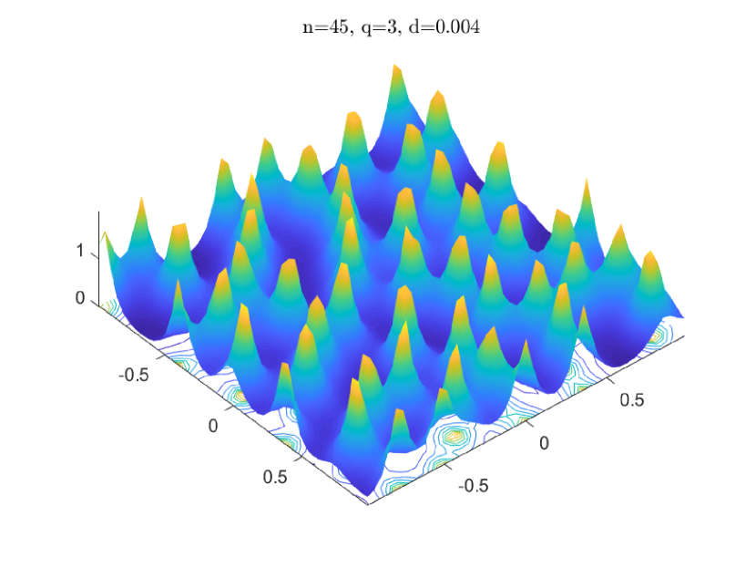
(a)

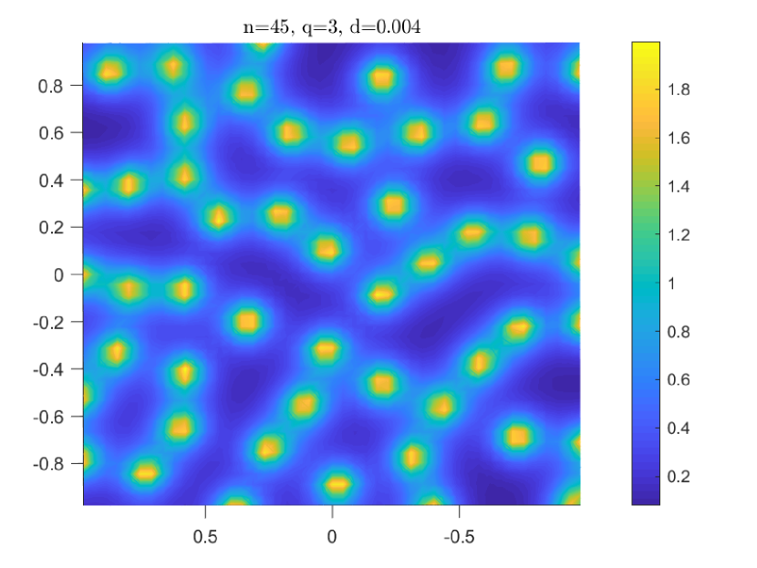
(b)

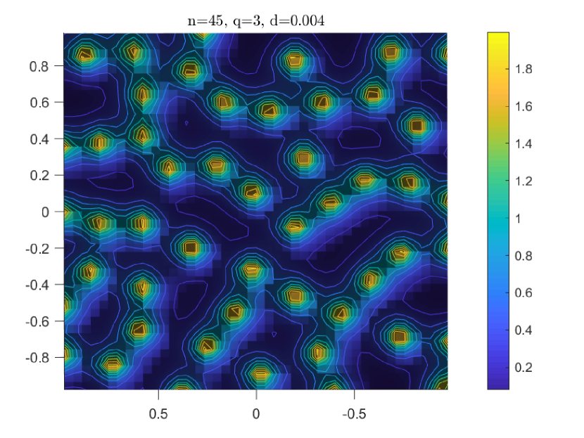
(c)

Figure 3: Numerical simulation of problem (2) with $q=3$, $d=0.004$, and $N=45$

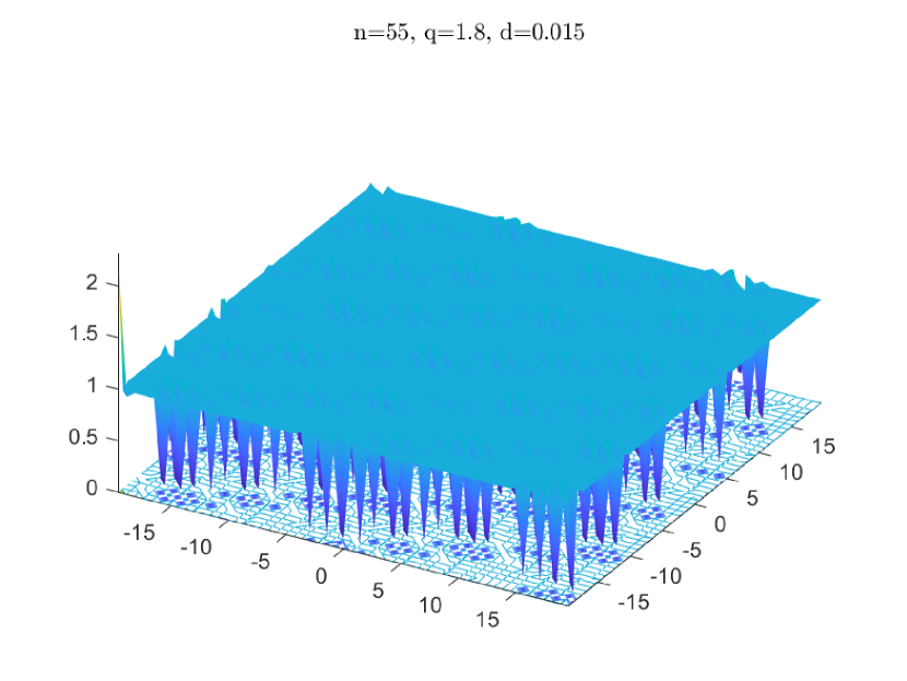
(a)

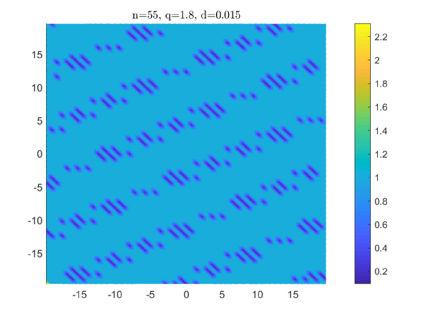
(b)

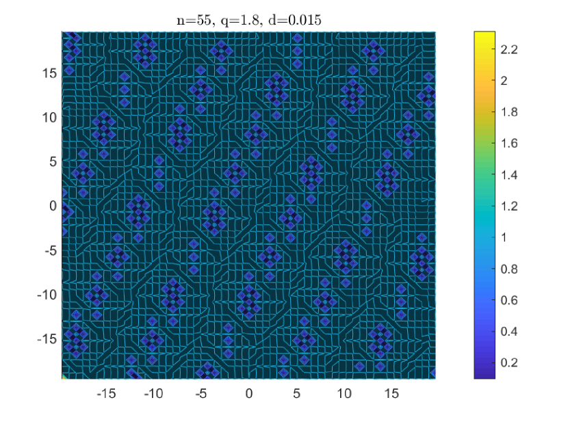
(c)

Figure 4: Numerical simulation of problem (2) with $q=1.8$, $d=0.015$, and $N=55$

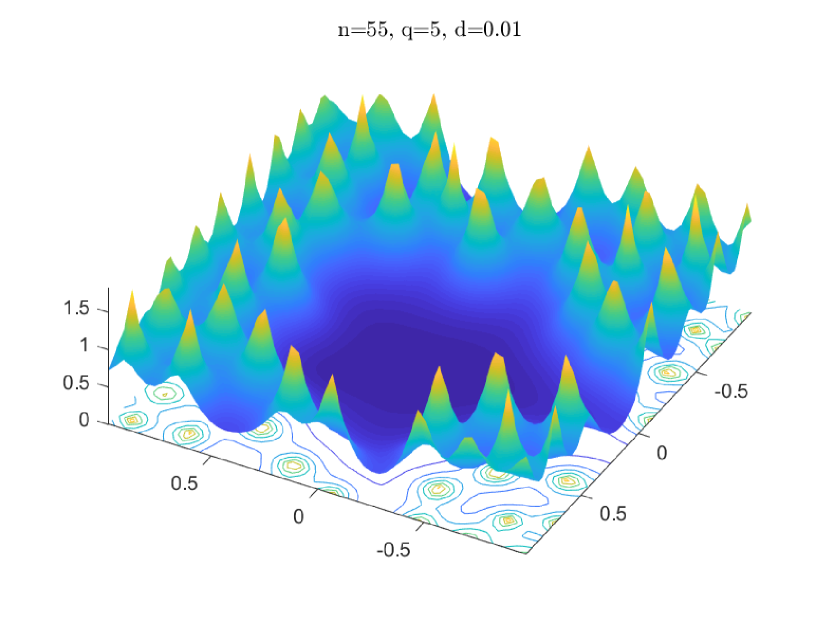
(a)

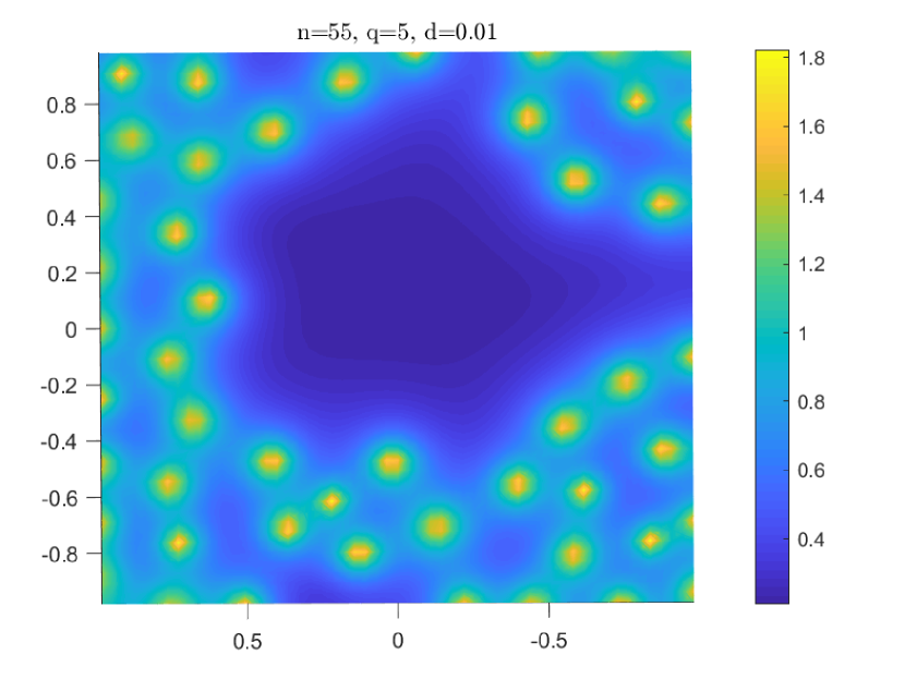
(b)

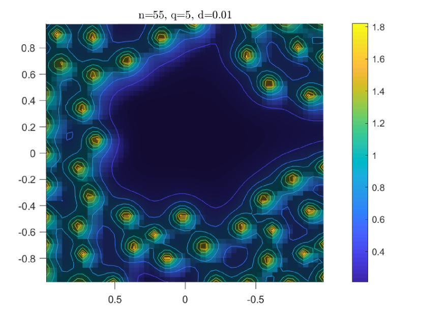
(c)

Figure 5: Numerical simulation of problem (2) with $q=5$, $d=0.01$, and $N=55$

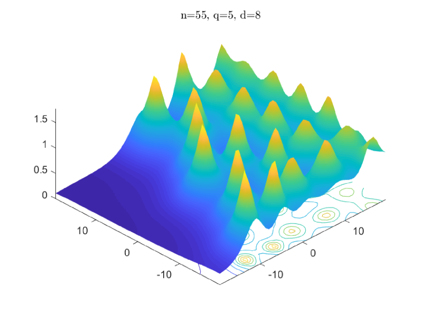
(a)

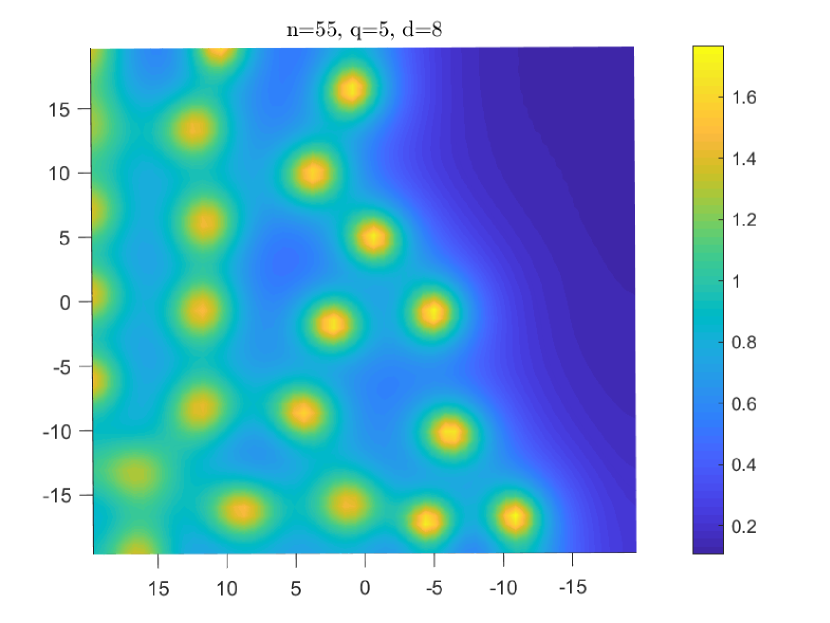
(b)

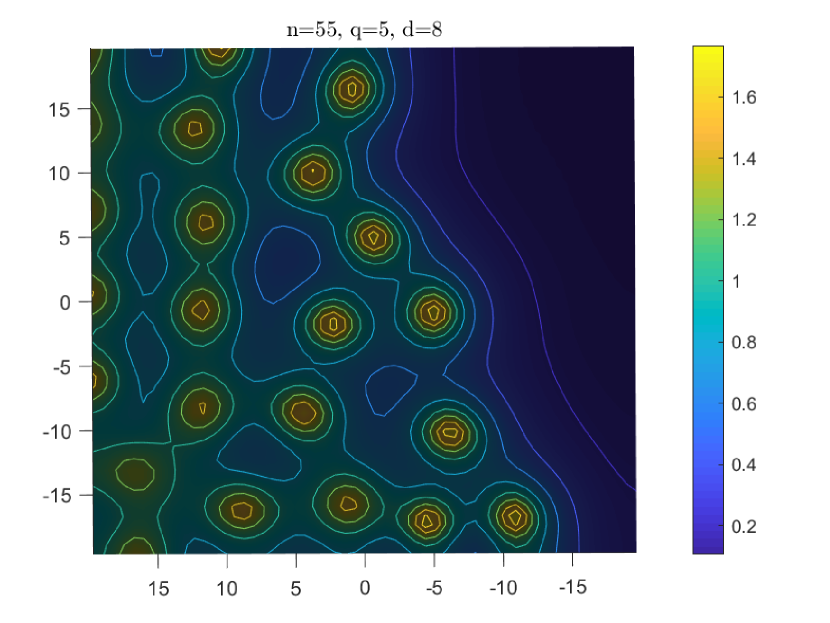
(c)

Figure 6: Numerical simulation of problem (2) with $q=5$, $d=8$, and $N=55$

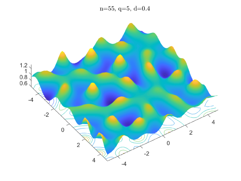
(a)

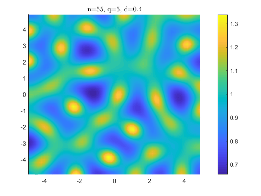
(b)

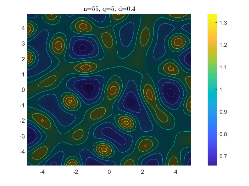
(c)

Figure 7: Numerical simulation of problem (2) with $q=5$, $d=0.4$, and $N=55$

On the other hand, Figure 8 shows a singular solution for $q=10$, $N=45$, and the initial vector $(X_{0})_{S}=|\cos(S)|,\,S=\overline{1,N^{2}}$. The domain $\Omega$ is successively selected as $[-10,10]^{2}$, $[-5,5]^{2}$, and $[-2,2]^{2}$ that lead to choosing the values of $d$ as $5.4$, $1.3$, and $0.21$ respectively. A single-peaked solution has been obtained for the parameters $q=55.6$, $d=0.13$, in the domain $\Omega=[-1,1]^{2}$ with a uniform mesh $N=22$; the initial vector has been taken as $(X_{0})_{S}=1/|\operatorname{Ssi}(S)|,\,S=\overline{1,N^{2}}$. The simulation solution is presented in Figure 9. It should be mentioned that the peak ridge reaches approximately $2.12\times 10^{5}$ at the point $(0.5,0.2273)$. By contrast, Figure 10 exhibits a simulation solution with nine peaks, four of which are located on a straight line in the diagonal center of the domain $\Omega=[-10,10]^{2}$ and the other ones are found on parallel straight lines on the left and right sides of the diagonal line. This graph has been computed for $q=100,d=14$ with a uniform mesh $N=20$, and the initial vector $(X_{0})_{S}=|\operatorname{cd}(S,10)|,\,S=\overline{1,N^{2}}$. Finally, a down multi-peaked solution is obtained in Figure 11 for the values $q=200$, $d=16$, and a uniform mesh $N=20$ of the domain $\Omega=[-10,10]^{2}$, whereas the initial vector is taken as $(X_{0})_{S}=1/|\operatorname{cn}(S,20)|,\,S=\overline{1,N^{2}}$.

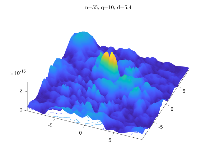
(a)

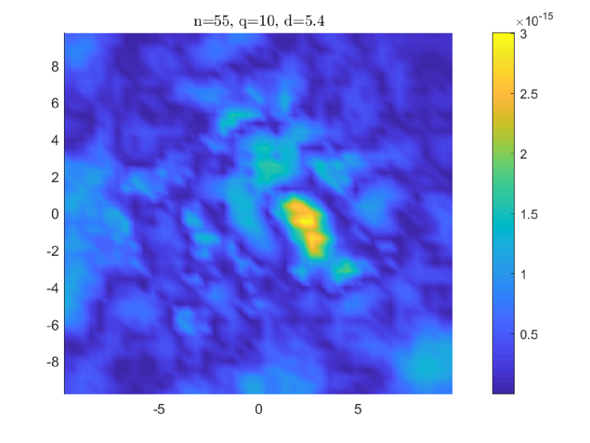
(b)

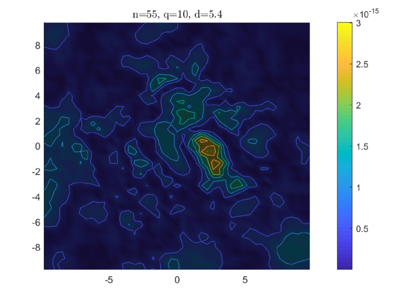
(c)

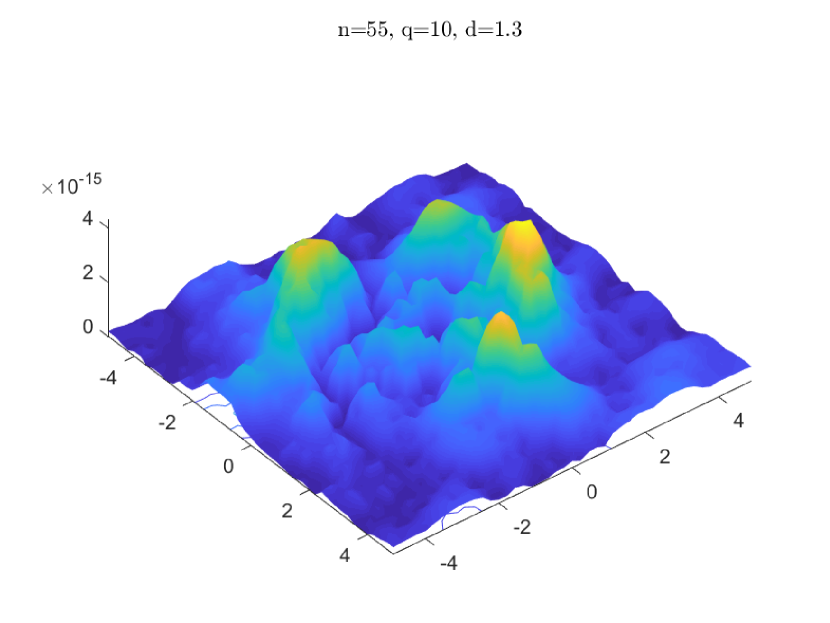
(d)

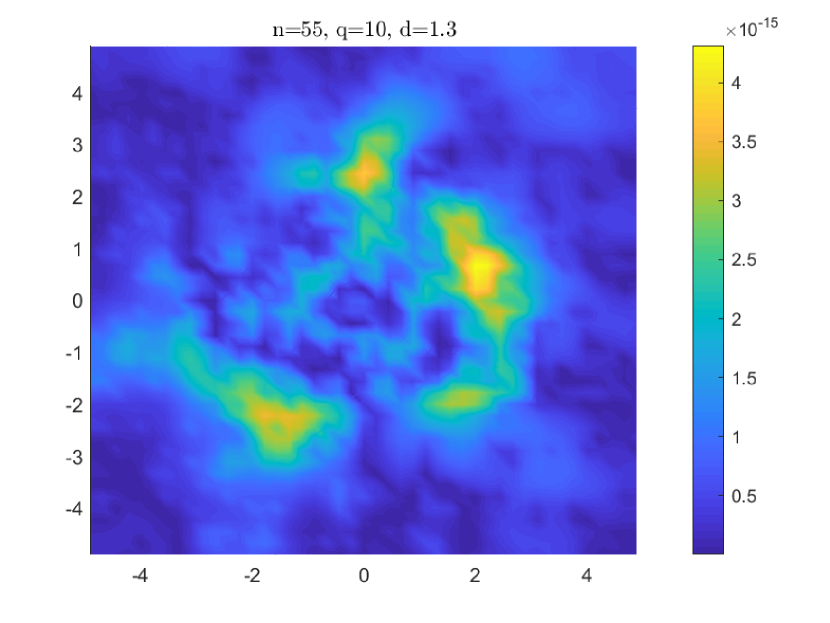
(e)

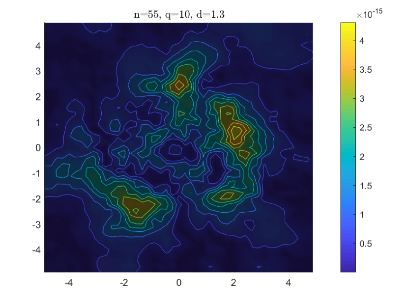
(f)

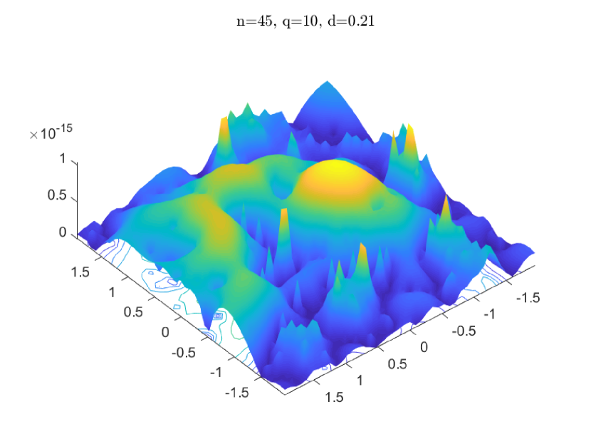
(g)

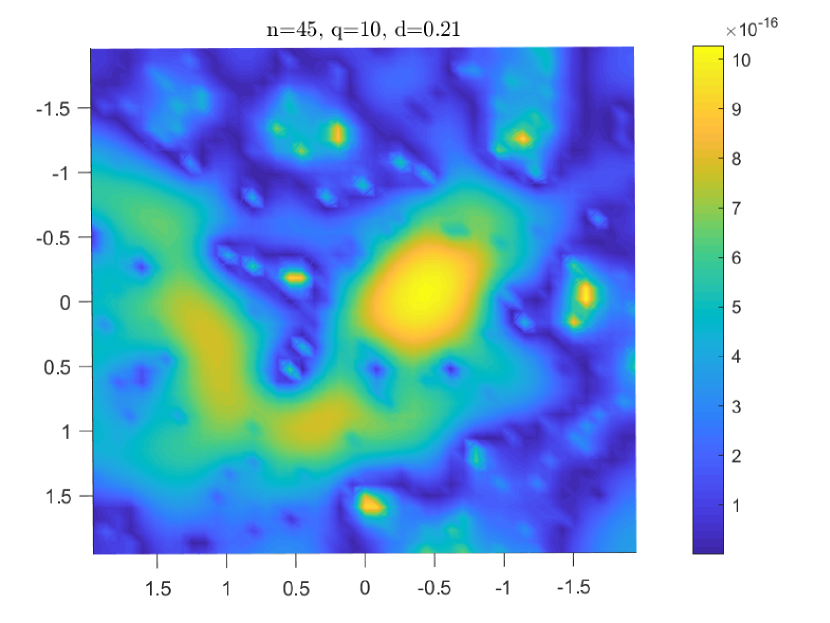
(h)

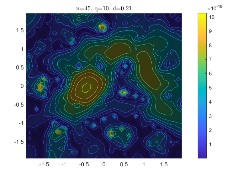
(i)

Figure 8: Numerical simulation of problem (2) with $q=10$, $n=45$, and different domains.

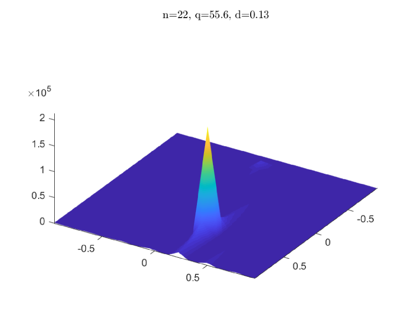
(a)

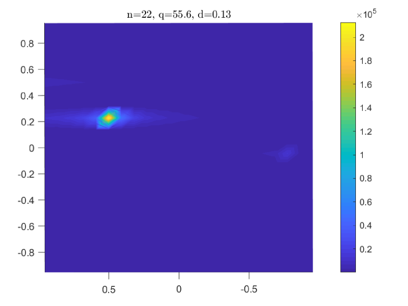
(b)

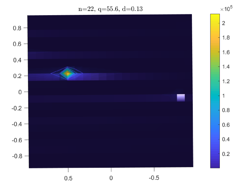
(c)

Figure 9: Numerical simulation of problem (2) for $q=55.6$, $d=0.13$, and $n=22$

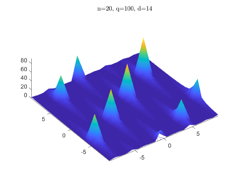
(a)

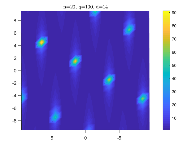
(b)

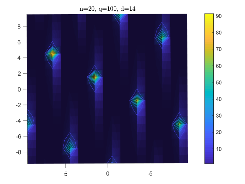
(c)

Figure 10: Numerical simulation of problem (2) for $q=100$, $d=14$, and $n=20$

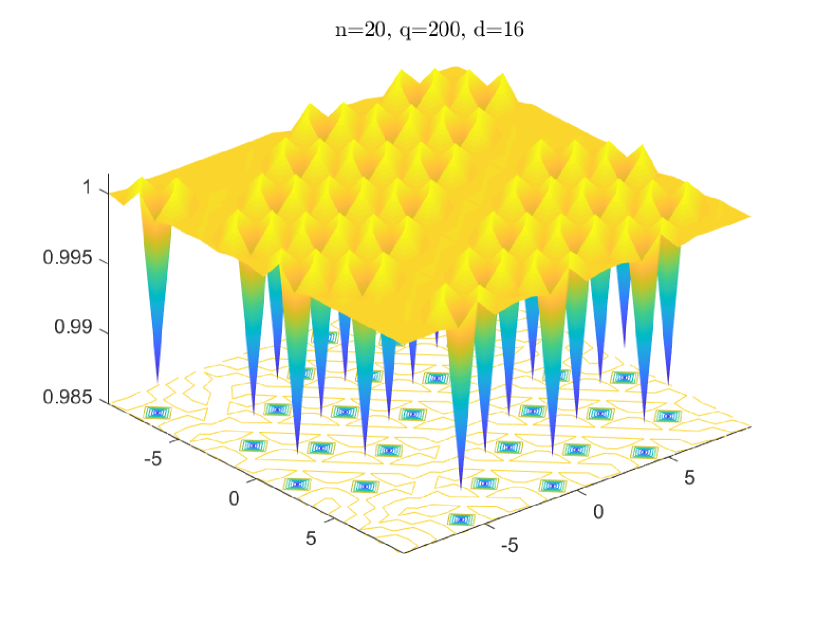
(a)

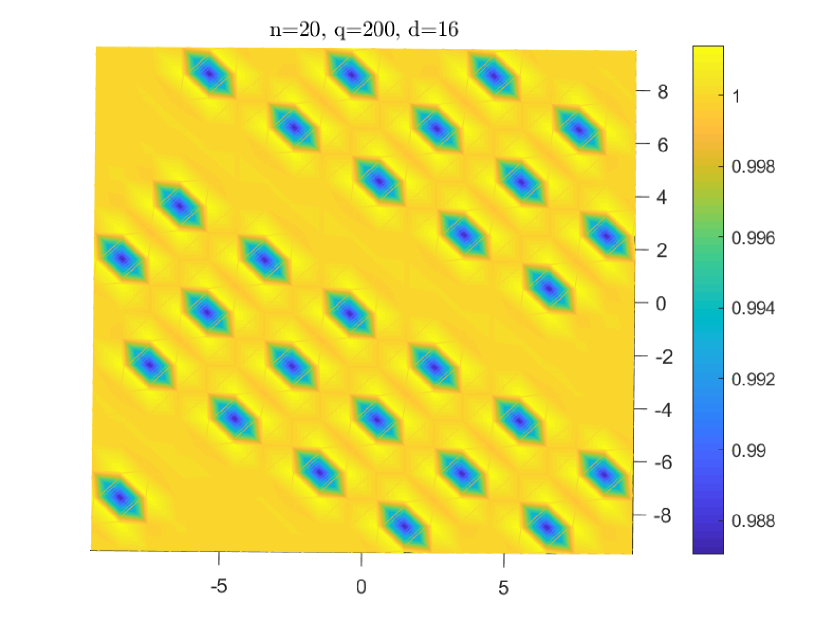
(b)

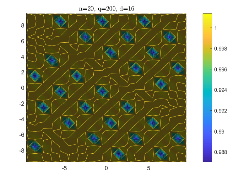
(c)

Figure 11: Numerical simulation of problem (2) for $q=200$, $d=16$, and $n=10$

4 Conclusion

In this paper, our primary aim was to create a proficient numerical algorithm for solving the problem (2), to investigate the discrete solution and to represent the solutions in $3$D and contour plots. To achieve this objective, we introduced a discrete iterative technique using the finite volume approach. The novel computed results that show single-peaked and multi-peaked solutions are concurred with the theoretical predictions in the literature. Our results will motivate future analytical and numerical results on the problem.

Data availability statement

Not applicable.

funding statement

Not applicable.

conflict of interest disclosure

No conflict of interest disclosure.

References

- [1] N. Ackermann, Multiple single-peaked solutions of a class of semilinear Neumann problems via the category of the domain boundary, Calc. Var. Partial Differential Equations, 7, 263–292, 1998.
- [2] D. Cao, and T. Küpper, On the existence of multi-peaked solutions to a semilinear Neumann problem, Duke Math. J., 97, 261–300, 1999.
- [3] R. Eymard, T. Gallouët, and R. Herbin, Finite volume methods, in Handbook of numerical analysis, Vol. VII, 713-1020, Handb. Numer. Anal., VII, North-Holland, Amsterdam, 2000.
- [4] M. Grossi, Uniqueness of the least-energy solution for a semilinear Neumann problem, Proc. Amer. Math. Soc., 128, 1665–1672, 1999.
- [5] C. Grossmann, H.G. Roos, and M. Stynes, Numerical treatment of partial differential equations, Springer, 2005.
- [6] T. Hillen, and K.J. Painter, A user’s guide to PDE models for chemotaxis, J. Math. Biol., 58, 183–217, 2009.
- [7] T.M. Hwang, and W. Wang, Analyzing and visualizing a discretized semilinear elliptic problem with Neumann boundary conditions, Numer. Methods Partial Differential Equations, 18, 261–279, 2002.
- [8] E.F. Keller, and L.A. Segel, Initiation of slime mold aggregation viewed as an instability, J. Theoret. Biol., 26, 399–415, 1970.
- [9] M.K. Kwong, Uniqueness of positive solutions of in , Arch. Ration. Mech. Anal., 105, 243–266, 1989.
- [10] C.C. Lee, Z.A. Wang, and W. Yang, Boundary-layer profile of a singularly perturbed nonlocal semi-linear problem arising in chemotaxis, Nonlinearity, 33, 5111–5141, 2020.
- [11] C.S. Lin, W. M. Ni, and L. Takagi, Large amplitude stationary solutions to a chemotaxis system, J. Differential Equations, 72, 1–27, 1988.
- [12] F.H. Lin, W. M. Ni, and J.C. Wei, On the number of interior peak solutions for a singularly perturbed Neumann problem, Commun. Pure Appl. Math., 60, 252–281, 2007.
- [13] H. Meinhardt, Models of Biological Pattern Formation, Academic Press, 1982.
- [14] F. Moukalled, L. Mangani, and M. Darwish, The Finite Volume Method in Computational Fluid Dynamics-An Advanced Introduction with OpenFOAM® and Matlab, Fluid Mechanics and Its Applications, Springer, 2016.
- [15] W.M. Ni, and I. Takagi, On the shape of least-energy solutions to a semilinear Neumann problem, Commun. Pure Appl. Anal., 44, 819–851, 1991.
- [16] W.M. Ni, and I. Takagi, Locating the peaks of least-energy solutions to a semilinear Neumann problem, Duke Math. J., 70, 247–281, 1993.
- [17] W.M. Ni, and I. Takagi, Diffusion, cross-diffusion, and their spike-layer steady states, Notices Amer. Math. Soc., 70, 9–18, 1998.
- [18] Z.Q. Wang, On the existence of multiple, single-peaked solutions for a semilinear Neumann problem,Arch. Ration. Mech. Anal., 120, 375–399, 1992.
- [19] J. Wei, On the interior spike layer solutions to a singularly perturbed Neumann problem, Tohoku Math. J. (2), 50, 159–178, 1998.