Converging TDDFT calculations in 5 iterations with minimal auxiliary preconditioning

Abstract

Eigenvalue problems and linear systems of equations involving large symmetric matrices are commonly solved in quantum chemistry using Krylov space methods, such as the Davidson algorithm. The preconditioner is a key component of Krylov space methods that accelerates convergence by improving the quality of new guesses at each iteration. We systematically design a new preconditioner for time-dependent density functional theory (TDDFT) calculations based on the recently introduced TDDFT-ris semiempirical model by re-tuning the empirical scaling factor and the angular momenta of a minimal auxiliary basis. The final preconditioner produced includes up to $d$-functions in the auxiliary basis and is named “rid”. The rid preconditioner converges excitation energies and polarizabilities in 5-6 iterations on average, a factor of 2-3 faster than the conventional diagonal preconditioner, without changing the converged results. Thus, the rid preconditioner is a broadly applicable and efficient preconditioner for TDDFT calculations.

1 Introduction

Eigenvalue problems and linear systems of equations involving large symmetric matrices are ubiquitous in quantum chemistry. By large, we refer to matrices that are too large to be explicitly stored in memory or on disk. Such problems appear as rate-limiting steps in a variety of contexts. For example, correlation energies within configuration interaction methods are obtained as eigenvalues of a large Hamiltonian matrix with dimensions of up to trillions of Slater determinants.^{1, 2, 3, 4, 5} Within response theory, excitation energies are obtained as eigenvalues of a response operator and (non)linear properties require the solution of linear systems of equations with respect to the response matrix; this response matrix has linear dimensions that scale at the least as $\mathcal{O}(N^{2})$ where $N$ is some measure of system size, such that storage of the full response matrix would require at least $\mathcal{O}(N^{4})$ storage. ^{6, 7, 8} Similarly, stability analyses of self-consistent-field solutions reduce to computing eigenvalues of orbital rotation Hessians.^{9, 10, 11}

The Krylov subspace approach is one of the most widely used and most successful strategies for iteratively computing a few extremal eigenpairs or solving linear equations in quantum chemistry.¹² Methods based on Krylov subspace approaches forego the need to store large matrices by centering the algorithm on matrix-vector products, $\mathbf{A}\mathbf{V}$, which can be computed on-the-fly and can be highly optimized for specific methods.¹² The eigenpairs are then written in terms of a small subspace, referred to as the Krylov subspace, which is expanded in each iteration. For most applications in quantum chemistry, the largest bottleneck by far is the calculation of matrix-vector products. Hence, significant effort has gone into accelerating these matrix-vector product routines, including through screening techniques,^{13, 14, 15} tensor decomposition techniques,^{16, 17} and hardware acceleration.^{18, 19}

The number of matrix-vector products needed is determined by how the Krylov subspace is expanded in each iteration. This step is referred to as the preconditioning step, and the efficiency of a Krylov subspace method is largely determined by the efficiency of the preconditioner. However, comparatively less effort has gone into designing efficient preconditioners. The major advantage to improving the preconditioner is that it does not change the final converged result of the Krylov subspace method. In addition, it remains compatible with other approaches to accelerating the matrix-vector product routines mentioned above. Thus, in this paper, we will focus on accelerating the Krylov subspace method by designing powerful preconditioners.

For quantum chemistry applications, we seek preconditioners that i) are significantly less expensive to apply than the original matrix to ensure that the overall computational cost is reduced, and ii) do not require system-specific tuning (although they will inevitably be method specific). In our previous research, we showed that semiempirical models are attractive preconditioners because they are typically several orders of magnitude cheaper than corresponding ab initio methods, can be broadly applicable, and often contain the most essential ingredients of the underlying physics.²⁰ We demonstrated this by using the semiempirical simplified Tamm-Dancoff²¹ (sTDA) and simplified time-dependent density functional theory (sTDDFT) models as preconditioners for computing excitation energies and polarizabilities with ab initio TDDFT, which led to a factor of 1.6 speed up on average for excitation energies and a factor of 1.2 speed up on average for polarizabilities.²⁰ Although the speedup of excitation energies with sTDA/sTDDFT is already significant, we believe the modest speedup of the polarizabilities suggests that further improvements are possible with a semiempirical model that more accurately reproduces transition densities.

In this paper, we systematically design a preconditioner for TDDFT excitation energies and polarizability calculations based on the minimal auxiliary basis approach for TDDFT, TDDFT-ris, recently introduced by us.²² The TDDFT-ris model has the same basic structure as the sTDA model, but significantly outperforms the sTDA model in the accuracy of the excitation energies, with just 0.06 eV error relative ab initio TDDFT compared to 0.24 eV error for the sTDA model. In addition, the TDDFT-ris model shows exceptional accuracy in the UV-vis absorption spectra for small to medium-sized organic molecules, indicating the oscillator strengths (and hence transition densities) are more accurately captured than in sTDA/sTDDFT. Furthermore, the TDDFT-ris model has additional flexibility in its structure that enables a greater degree of design than would be possible with the sTDA model.

Thus, on account of its superior accuracy and flexibility, we anticipate that TDDFT-ris will be a powerful preconditioner for TDDFT excitation energies and polarizability calculations. The final preconditioner proposed in this paper, termed rid, converges excitation energies in 5-6 iterations on average and converges linear equations in about 6 iterations on average, compared to 12-17 iterations for excitation energies and 12-13 iterations for linear equations using the conventional diagonal preconditioner. Furthermore, the rid preconditioner all but erases the difference in the number of iterations needed to converge excitation energies with global hybrid vs range-separated hybrid functionals. We note that although it has been suggested that improving the preconditioner can paradoxically worsen the convergence of the algorithm,^{23, 24} we observe no such deterioration in practice.

This paper is organized as follows: In section 2, we briefly review the preconditioned Krylov subspace algorithm, as well as the working equations for ab initio TDDFT and the semiempirical TDDFT models used in this work. In section 3, we systematically design the rid preconditioner. In section 4, we evaluate the rid preconditioner by comparing its performance to the diagonal preconditioner and sTDA preconditioner when computing the excitation energies or polarizability. Finally, we conclude in section 5 by offering our perspective on how to make broadly applicable preconditioners for Krylov subspace methods.

2 Theory and Methods

2.1 Krylov Subspace Methods

Here, we briefly describe the framework of the semiempirical preconditioned Krylov subspace method, taking the Davidson algorithm as a representative example.¹² The goal of the Davidson algorithm is to find the $N_{\text{states}}$ lowest eigenvalues and corresponding eigenvectors of a Hermitian matrix $\mathbf{A}$. The Davidson algorithm works by iteratively expanding a subspace (called the Krylov subspace) spanned by a set of basis vectors until it contains the desired eigenpairs to a specified threshold. At the $k$-th iteration, the Krylov subspace is spanned by the columns of the matrix $\mathbf{V}^{(k)}$. Here, we assume the columns of $\mathbf{V}^{(k)}$ form an orthonormal basis, but that is not required.¹⁴ To accelerate convergence, the Davidson algorithm makes use of an approximation to $\mathbf{A}$—called the preconditioner and denoted here using $\mathbf{T}$—which will be used to i) generate the initial subspace, $\mathbf{V}^{(0)}$, and ii) generate expansion directions at each iteration. In conventional implementations, $\mathbf{T}=\mathbf{A}^{\text{diag}}$ is the diagonal approximation of $\mathbf{A}$. In this paper we will consider semiempirical models for $\mathbf{T}$.

The Davidson algorithm begins by generating the initial subspace, usually by using the low-lying eigenvectors of $\mathbf{T}$. In principle, so long as the true eigenvectors have a nonzero overlap with the initial subspace, then the Davidson algorithm will arrive at the correct solution. To help ensure this, additional initial vectors are often included in the initial subspace, i.e., $N_{\text{init}}>N_{\text{states}}$, where $N_{\text{init}}$ is the number of initial guesses. Regardless of how many initial vectors are used, in each iteration, the subspace projection of $\mathbf{A}$ is computed as

$$\mathbf{a}^{(k)}=\mathbf{V}^{(k),\dagger}\mathbf{A}\mathbf{V}^{(k)}.$$ (1)

The approximate eigenvalues are obtained from $\mathbf{a}^{(k)}$ by diagonalizing,

$$\mathbf{a}^{(k)}\mathbf{x}_{n}^{(k)}=\Omega_{n}^{(k)}\mathbf{x}_{n}^{(k)},$$ (2)

and the approximate eigenvectors are obtained from

$$\mathbf{X}^{(k)}=\mathbf{V}^{(k)}\mathbf{x}^{(k)}.$$ (3)

Next, for each root, the residual is computed according to

$$\mathbf{R}_{n}^{(k)}=\mathbf{A}\mathbf{X}^{(k)}_{n}-\mathbf{X}^{(k)}_{n}\Omega_{n}^{(k)}.$$ (4)

If the residual norm, $|R_{n}^{(k)}|$, is smaller than a user-defined threshold then that eigenpair is considered converged. For each unconverged eigenpair, the residual is preconditioned to generate new search directions,

$$\mathbf{v}_{n}^{(k+1)}=(\mathbf{T}-\Omega_{n}^{(k)})^{-1}\mathbf{R}_{n}^{(k)}.$$ (5)

Thus, the $\mathbf{T}$ should be chosen such that applying a shifted inverse is inexpensive relative to matrix multiplications of $\mathbf{A}$. When $\mathbf{T}$ is a diagonal matrix, the preconditioning step reduces to element-wise division. When $\mathbf{T}$ is a semiempirical model, we solve Eq. (5) using an inner Krylov subspace method. Finally, the new search directions are orthogonalized against $\mathbf{V}^{(k)}$ and each other using the modified Gram-Schmidt procedure, and then appended to $\mathbf{V}^{(k)}$ to form $\mathbf{V}^{(k+1)}$. The algorithm is depicted schematically in Fig. 1.

It has been argued that the step in Eq. (5) should not be considered a preconditioning step because if we replace $\mathbf{T}$ with $\mathbf{A}$, then no update vector is produced.²³ This can be seen by inserting Eq. (4) into (5), which gives $\mathbf{v}_{n}^{(k+1)}=\mathbf{X}_{n}^{(k)}$. This result has been used to argue that improving the preconditioner in the Davidson algorithm can lead to stagnation, not acceleration.^{23, 24, 3} Indeed, the Jacobi-Davidson algorithm was proposed to avoid the stagnation of the Davidson algorithm.^{23, 24} However, despite these strong theoretical arguments, observation of this stagnation in practical quantum chemistry calculations remains elusive.^{25, 26} The solution to this apparent paradox comes from the choice to initiate the algorithm with an eigenvector of $\mathbf{T}$, which has two consequences for the stability of the algorithm. First, somewhat trivially, if $\mathbf{T}$ was indeed identical to $\mathbf{A}$, then the residual would be zero in the first step and there would be no need to precondition. Second, including low-lying eigenvectors of $\mathbf{T}$ in the initial subspace guarantees that the $\mathbf{T}-\Omega_{n}^{(k)}$ is not singular, and leads to nearly identical behavior between the Davidson and Jacobi-Davidson algorithms in practice.²⁷

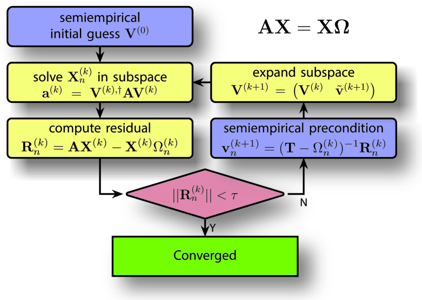
Figure 1: The scheme of Davidson algorithm with semiempirical preconditioning.

2.2 Time-dependent density functional theory

For the remainder of this paper, labels $i,j$ will be used to denote occupied orbitals, and $a,b$ will be used to denote virtual orbitals, and $p,q,r,s$ will be used to denote generic orbitals.

2.2.1 ab initio TDDFT

Excitation energies within linear response TDDFT are found by solving the symplectic eigenvalue problem

$$\begin{pmatrix}\mathbf{A}&\mathbf{B}\\ \mathbf{B}&\mathbf{A}\end{pmatrix}\begin{pmatrix}\mathbf{X}_{n}\\ \mathbf{Y}_{n}\end{pmatrix}=\Omega_{n}\begin{pmatrix}\mathbf{1}&\mathbf{0}\\ \mathbf{0}&\mathbf{-1}\end{pmatrix}\begin{pmatrix}\mathbf{X}_{n}\\ \mathbf{Y}_{n}\end{pmatrix},$$ (6)

where

$$(A+B)_{ia,jb}= (\varepsilon_{a}-\varepsilon_{i})\delta_{ab}\delta_{ij}+2f^{\text{xc}}_{iajb}+2(ia|jb)$$

$$-c_{x}[(ib|ja)+(ij|ab)],$$ (7a)

$$(A-B)_{ia,jb}= (\varepsilon_{a}-\varepsilon_{i})\delta_{ab}\delta_{ij}+c_{x}[(ib|ja)-(ij|ab)],$$ (7b)

are the electric and magnetic orbital rotation Hessians, respectively, $\varepsilon_{p}$ is the Kohn-Sham eigenvalue associated with Kohn-Sham orbital $\phi_{p}$, $f^{\text{xc}}_{iajb}$ is a matrix element of the exchange-correlation kernel,

$$(pq|rs)=\iint dxdx^{\prime}\phi_{p}(x)\phi_{q}(x)\frac{1}{|x-x^{\prime}|}\phi_{r}(x^{\prime})\phi_{s}(x^{\prime})$$ (8)

is an electron repulsion integral (ERI), and $c_{x}$ denotes the Hartree–Fock mixing coefficient. The eigenvectors, $|X_{n},Y_{n}\rangle$, represent transition densities.

In this paper, we focus on excitation energies within the Tamm–Dancoff Approximation, which is obtained by setting $\mathbf{B}=0$ in the above, thus reducing to the Hermitian eigenvalue problem

$$\mathbf{A}\mathbf{X}_{n}^{\text{TDA}}=\Omega_{n}^{\text{TDA}}\mathbf{X}_{n}^{\text{TDA}}.$$ (9)

The TDDFT dynamic polarizability at frequency $\omega$ is computed as

$$\alpha_{vu}^{\text{TDDFT}}(\omega)=\begin{pmatrix}\boldsymbol{\mu}^{v}_{\text{vo}}\\ \boldsymbol{\mu}^{v}_{\text{ov}}\end{pmatrix}^{\dagger}\left[\begin{pmatrix}\mathbf{A}&\mathbf{B}\\ \mathbf{B}&\mathbf{A}\end{pmatrix}-\omega\begin{pmatrix}\mathbf{1}&\mathbf{0}\\ \mathbf{0}&\mathbf{-1}\end{pmatrix}\right]^{-1}\begin{pmatrix}\boldsymbol{\mu}^{u}_{\text{vo}}\\ \boldsymbol{\mu}^{u}_{\text{ov}}\end{pmatrix},$$ (10)

where the $\boldsymbol{\mu}_{\text{vo}}^{v}$ and $\boldsymbol{\mu}_{\text{ov}}^{v}$ are the virtual-occupied and occupied-virtual blocks matrix representation of the dipole moment operator in the $v$ direction, respectively.

2.2.2 Semiempirical TDDFT models

In recent years several semiempirical models have been developed to approximate TDDFT that retain the ab initio Kohn-Sham reference but use semiempirical approximations to the linear response function. Here, we focus on the simplified TDA/TDDFT^{21, 28} (sTDA/TDDFT) and the TDDFT-ris models as these were explicitly designed for use with hybrid density functionals. The results here are expected to apply to semiempirical models that focus on semilocal density functionals as well, such as TDDFT+TB²⁹ and TDDFT-as.³⁰

TDDFT-ris and sTDA are both constructed similarly by i) neglecting the exchange-correlation kernel, i.e., setting $f^{\text{xc}}=0$, and ii) approximating the 4-index ERIs with a contraction of 2-index and 3-index tensors in Eq. (8),

$$(pq|rs)\approx\sum_{PQ}K_{pq}^{P}J_{PQ}K_{rs}^{Q}.$$ (11)

It is the definition of these three tensors that distinguishes the TDDFT-ris and sTDA.

In TDDFT-ris, ERIs are approximated using the resolution of the identity (RI) approximation with a minimal auxiliary basis such that

$$K_{pq}^{P}=(pq|P),\quad J_{PQ}=(P|Q)^{-1},$$ (12)

where $P$, $Q$ label auxiliary basis functions and $(pq|P)$ and $(P|Q)$ are the three-center and two-center ERIs, respectively.^{31, 32, 33, 16, 34, 35, 36, 37, 38} The auxiliary basis functions are Gaussians with exponents defined by the element type, $A$, as

$$\alpha_{A}=\frac{\theta}{R_{A}^{2}},$$ (13)

where $R_{A}$ is the atomic radius tabulated by Ghosh et al,³⁹ and $\theta$ is a global scaling factor. Previously, we chose $\theta=0.2$ by minimizing the error in excitation energies and absorption spectra.²² In our previous work, we exclusively used $s$-type functions in the auxiliary basis, but here we will explore the impact of including higher angular momentum functions as well.

In sTDA, the ERIs are approximated using parametrized transition monopoles with

$$K_{pq}^{A}=\sum_{\nu\in A}C^{\prime}_{\nu p}C^{\prime}_{\nu q},\quad J_{AB}=\Gamma_{AB}$$ (14)

where $\nu\in A$ indicates atomic orbitals centered on atom $A$, $\mathbf{C}^{\prime}$ is the Löwdin orthogonalized molecular orbital coefficient matrix, and $\Gamma_{AB}$ is a damped Coulomb operator between atoms $A$ and $B$ of the form

$$\Gamma_{AB}=\left((R_{AB})^{y}+(c_{y}\eta_{AB})^{-y}\right)^{-\frac{1}{y}}$$ (15)

where $R_{AB}$ is the distance between the two atoms $A$ and $B$, $y$ is an empirically tuned parameter, $c_{y}$ is either 1 or the HFX mixing coefficient, and $\eta_{AB}$ is the average chemical hardness. Separate $\Gamma$ functions are used for the Coulomb and exchange terms with independently tuned empirical parameters. Here we only use the default suggested parameters for the density functionals used.^{21, 40} To be clear, by sTDA/sTDDFT model here, we specifically refer to the approximation to the $\mathbf{A}$ and $\mathbf{B}$ matrices used in sTDA/sTDDFT. We note that the sTDA method as implementd in the sTDA program includes additional innovations, such as a configuration state function selection algorithm and perturbative corrections.²¹

2.3 Implementation details

We implemented the algorithms described above in a pilot python code. In our implementation, the ground-state Kohn-Sham reference, matrix-vector product subroutines with density fitting, and all ERIs are provided by PySCF 2.3.0.⁴¹ The matrix-vector products for sTDA and ris-type preconditioners are implemented in Python.²²

3 Systematic Design of the rid Preconditioner

One of the strong advantages of the TDDFT-ris method over competing semiempirical methods is that it can be straightforwardly extended to include atomic multipoles by adding higher angular momentum functions (e.g., $p$ and $d$ functions) to the auxiliary basis.²² In this section, we exploit the flexibility of the TDDFT-ris model to systematically design an optimal TDDFT preconditioner. The TDDFT-ris model has two essential design choices: i) the global scale factor $\theta$ used to determine the exponents for the auxiliary basis, and ii) the maximum angular momentum used in the auxiliary basis. In our previous work, we chose $\theta=0.2$ and used only $s$-type functions. However, we do not expect the same parameters to necessarily be optimal for preconditioning as well. Furthermore, we expect these two design choices to be correlated. For example, the appearance of an optimal $\theta$ was previously attributed to engineered error cancellation between the approximated Coulomb contribution and the neglected exchange-correlation kernel.²² Thus, improving the description of the Coulomb energy may require a different $\theta$ to maintain the error cancellation. Finally, we have the additional constraint that the semiempirical $\mathbf{T}$ must remain significantly less expensive to apply than $\mathbf{A}$ so that the computational time saved by preconditioning is not simply spent in the preconditioner instead.

We proceed by first exploring strategies to contain the cost of the preconditioners without sacrificing efficacy. Next, we will explore the performance of preconditioners with different maximum angular momenta, while tuning $\theta$ within the range of 0.1–10. As a benchmark, we compute the lowest 5 excited states using the PBE0 density functional⁴² with the def2-SVP basis set⁴³ for the TUNE8 set, which is a subset of the PRECOND19 set defined previously²⁰ and repeated in the Supporting Information. We choose a convergence threshold of $10^{-5}$ for the residual norm. As a figure of merit in this section we focus on the average number of ab initio matrix-vector products, $N_{\text{mv}}$.

3.1 Controlling the preconditioning cost

To avoid the preconditioner becoming the bottleneck of the algorithm, we target a preconditioning cost on the order of 1-2% of the overall wall time, meaning that one matrix-vector multiplication using $\mathbf{T}$ needs to be about $10^{3}$ times faster than a matrix-vector multiplication using $\mathbf{A}$. We focus our efforts on the exchange terms because for both TDDFT-ris and sTDA, the exchange contribution of the matrix-vector products scale as $\mathcal{O}(N^{4})$, where $N$ is the number of basis functions. We introduce an energy cutoff for the exchange ERIs, $t_{\text{cut}}$, and neglect all ERIs involving virtual molecular orbitals (MOs) higher in energy than $\epsilon_{\text{HOMO}}+t_{\text{cut}}$ or occupied MOs lower in energy than $\epsilon_{\text{LUMO}}-t_{\text{cut}}$, where HOMO stands for highest occupied molecular orbital and LUMO, lowest unoccupied molecular orbital. We find that $t_{\text{cut}}=40$ eV allows us to dramatically reduce the cost of applying $\mathbf{T}$ without significantly increasing the $N_{\text{mv}}$. We do not truncate any MOs for the Coulomb terms because they are much less expensive than the exchange terms, scaling as $\mathcal{O}(N^{3})$, and because truncation deteriorates the preconditioning efficiency. Finally, we reduce the time spent in the iterative preconditioning steps by using a loose convergence threshold of $10^{-2}$ and by setting a maximum number of iterations of 20. The convergence threshold for initial guesses is set to $10^{-3}$.

3.2 The impact of the maximum angular momentum

In this section we test the performance of a series of 6 ris-type preconditioners with maximum angular momentum up to d functions on non-hydrogen atoms. In addition, we test using different maximum angular momentum values for Coulomb and for exchange bases. The preconditioners are labeled as $(\ell_{J},\ell_{K})$, where $\ell_{J}$ and $\ell_{K}$ are the maximum angular momenta used for the Coulomb and exchange terms, respectively. For example, the $(p,d)$ preconditioner uses up to $p$ functions for the Coulomb terms and up to $d$ functions for the exchange terms. The average $N_{\text{iter}}$ across TUNE8 is shown for all 6 preconditioners as a function of $\theta$ in Fig. 2. As comparison, the average $N_{\text{mv}}$ using the diagonal preconditioner is 50.5. From this figure, we first see that there is indeed a slight dependence of the optimal $\theta$ on the maximum angular momentum. The preconditioner with only $s$ functions is relatively insensitive to the value of $\theta$ but has maximum performance with $\theta=4$. By contrast, the optimal $\theta$ found by tuning the energetics and spectra was 0.2.²² Preconditioners with up to $p$ functions, on the other hand, have an optimal $\theta$ of 2.0, while preconditioners with up to $d$ functions have an optimal $\theta$ of 0.6. Next, we see that the performance of the preconditioners tends to improve with the addition of angular momentum. The optimal $s$-only preconditioner has an average $N_{\text{mv}}$ of 31.5, while the best $p$-type and $d$-type preconditioners reduce this to 26.6 and 24.8, respectively. Finally, we find, somewhat fortuitously, that the preconditioning performance is essentially ambivalent about the angular momentum used for the exchange terms. For example, the optimal $(p,s)$ type and $(p,p)$ type preconditioners use $N_{\text{mv}}$ of 26.6 and 26.8, respectively. Similarly, the optimal $(d,s)$, $(d,p)$, and $(d,d)$ preconditioners have $N_{\text{mv}}$ of 25.0, 24.8, and 24.8, essentially identical performance.

We do not consider higher angular momentum functions because the $d$-type preconditioners are already nearly optimal. To demonstrate this, we used the full auxiliary basis as a preconditioner. The full auxiliary basis would be an impractical preconditioner, but it can show the upper limit of what can be achieved with a preconditioner that neglects $f^{\text{xc}}$. With the full auxiliary basis, the test suite converges with $N_{\text{mv}}=23$ (see Fig. 2), only reducing the $(d,s)$ result by 2 matrix-vector products or 8%.

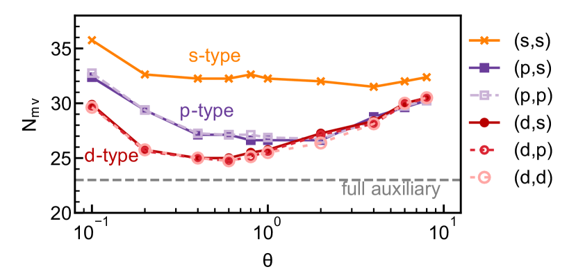
Figure 2: The average $N_{\text{mv}}$ obtained from computing lowest 5 states with PBE0/def2-SVP on TUNE8 set using different ris-type preconditioners. The label $(\ell_{J},\ell_{K})$ indicates a preconditioner using up to $\ell_{J}$ functions for the Coulomb terms and up to $\ell_{K}$ functions for the Exchange terms. For comparison, the dashed horizontal line shows the average $N_{\text{mv}}$ obtained using the full auxiliary basis as a preconditioner.

Based on these results, we propose the $(d,s)$ preconditioner with $\theta=0.6$ as our best performing preconditioner, and name it rid. With this structure, the total cost of preconditioning is much less than 1% of the overall algorithm. As a last step for creating the rid preconditioner, we re-tune the number of initial guesses used to initiate the Davidson algorithm. We find that the performance of the rid preconditioner is maximized when using up to 3 additional initial guesses. That is, we generate $N_{\text{init}}=N_{\text{states}}+\text{min}(N_{\text{states}},3)$ initial guesses for the Davidson algorithm. The diagonal and sTDA preconditioners, by contrast, are most effective when using 8 additional initial guesses. The detailed results of this tuning are shown in Fig. S1 in Supporting Information.

4 Evaluating the Rid Preconditioner

In this section, we benchmark the performance of the rid preconditioner in computing excitation energies and polarizabilities for small to medium sized molecules. We compare its efficacy to that of the diagonal preconditioner and the sTDA preconditioner using the PBE0⁴² and $\omega$B97X⁴⁴ density functionals with the def2-TZVP basis set.⁴³ For consistency, we employ the same set of 19 molecules from our previous study, referenced as PRECOND19.²⁰ This set comprises nanoparticle, organic dyes, chemical probes, and bioluminescent molecules (see the Supporting Information for the complete list of molecules in PRECOND19). For clarity, TUNE8 is a subset of PRECOND19. We use as figures of merit the number of iterations, $N_{\text{iter}}$, as well as the number of ab initio matrix-vector products, $N_{\text{mv}}$. The speedup factor, $\zeta_{\text{iter}}$ or $\zeta_{\text{mv}}$, is defined as the ratio of $N_{\text{iter}}$ or $N_{\text{mv}}$ for the diagonal preconditioner to that for the rid preconditioner. For example, $\zeta^{\text{rid}}_{\text{iter}}=N^{\text{diag}}_{\text{iter}}/N^{\text{rid}}_{\text{iter}}$. For tables with all the results shown in this section, see the Supporting Information.

The complete results of these benchmarks are summarized in Fig. 3, which shows a violin plot of all the observed speedups using the rid preconditioner relative to the diagonal preconditioner for both excitation energies and polarizabilities.

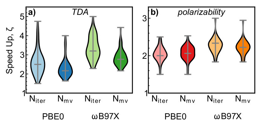
Figure 3: Violin plot of all observed speedups using the rid preconditioner for computing a) TDA excitation energies and b) polarizabilities. For each dataset, the median, minimum, and maximum observations are marked with a line.

4.1 TDA Excitation Energies

To benchmark excitation energies, we compute the lowest 1, 5, and 20 states, which are intended to mimic typical use cases of computing the optical gap, low-lying states, and a UV-vis spectrum, respectively. The complete results are shown in Fig. 4 and summarized in Table 1. For more detailed results, see the Supporting Information. Results using the full TDDFT equations (i.e., without the TDA) are similar and are collected in Fig. S2 of the Supporting Information.

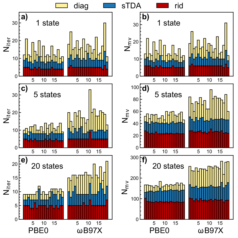
Figure 4: Performance of the diagonal, sTDA, and rid preconditioners for computing TDA excitation energies. Left three panels show the number of iterations ($N_{\text{iter}}$), while the right three panels show the matrix-vector products ($N_{\text{mv}}$) required to converge 1, 5 or 20 states.

Fig. 4 shows that the rid preconditioner systematically outperforms both the diagonal and the sTDA preconditioners. For every molecule considered here, the rid preconditioner converges faster than the sTDA preconditioner and the diagonal preconditioner. Using PBE0, all excitation energies converge in at most 6 iterations, and only 4.5 iterations on average. By contrast, all excitation energies required at least 7 iterations using the sTDA preconditioner (8.0 on average) and at least 9 iterations for the diagonal preconditioner (11.6 on average), meaning the worst-case performance of the rid preconditioner is better than the best-case performance of the conventional and sTDA preconditioners. The rid preconditioner reduces the number of iterations by a factor of 2.6 on average and up to a factor of 4.8, compared to a factor of 1.5 on average and 2.7 at best for the sTDA.

The results are similar using $\omega$B97X: the rid preconditioner converges in 5.2 iterations on average, compared to 9.8 for sTDA and 17.4 for the diagonal preconditioner. Thus, the rid preconditioner reduces the number of iterations by a factor of 3.4 on average and up to a factor of 5.0, compared to a factor of 1.8 on average and 3.3 at best for the sTDA. Moreover, the rid preconditioner all but erases the difference in the number of iterations required to converge $\omega$B97X compared to PBE0. For example, using the diagonal preconditioner, $\omega$B97X requires an additional 5.8 iterations than PBE0 on average, whereas with the rid preconditioner, only an additional 0.7 iterations is required.

Table 1: The range and the average number of iterations, $N_{\text{iter}}$, required to compute TDA excitation energies using the PBE0 and $\omega$B97X density functionals with diagonal, sTDA and rid preconditioners.

		PBE0			$\omega$B97X
precond.		diag	sTDA	rid	diag	sTDA	rid
$N_{\text{iter}}$	min.	9	7	4	11	8	4
	max.	21	11	6	33	14	9
	avg.	11.6	8.0	4.5	17.4	9.8	5.2
$\zeta_{\text{iter}}$	min.	–	1.1	1.5	–	1.2	2.3
	max.	–	2.7	4.8	–	3.3	5.0
	avg.	–	1.5	2.6	–	1.8	3.4

For a more detailed analysis of the convergence behavior, we consider the calculation of the first 5 excitation energies of fluorescein (5 in PRECOND19) using the $\omega$B97X functional. The maximum residual norm at each iteration of the Davidson algorithm is shown in Fig. 5. For this example, the rid preconditioner requires 5 iterations, the sTDA preconditioner requires 9 iterations, and the diagonal 18. From Fig. 5, we see that compared to the diagonal preconditioner, the rid algorithm is benefiting from both an improved initial guess and from a faster convergence rate. Consider the initial guesses first. In Fig. 5, we see that the diagonal preconditioner stagnates for the first 8 iterations before the residual norm begins to decrease exponentially (note the log scale), indicating that the algorithm is still searching for a suitable starting vector. By contrast, the sTDA and rid initial guesses show no such stagnation, because they immediately find suitable initial guesses. Furthermore, the rid initial guess has a sharply reduced initial residual norm (0.020) compared to sTDA (0.118) and the diagonal (0.139).

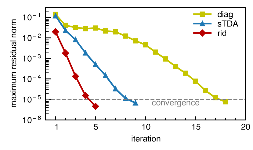
Figure 5: The convergence behavior of computing the lowest 5 TDA excitation energies of fluorescein using $\omega$B97X/def2-TZVP with the diagonal, sTDA, and rid preconditioners. The horizontal line at $10^{-5}$ shows the convergence threshold.

Next, consider the convergence rate. Each algorithm in Fig. 5 converges essentially exponentially once the residual norm falls below $10^{-2}$. We use this to estimate rates of convergence for each algorithm by fitting a line to the base 10 logarithm of the residual norm while it is in the range $10^{-2}$ to $10^{-5}$. The rid preconditioner has a remarkable slope of $-1.03$, meaning that the residual norm decreases by a factor of $10^{-1.03}=0.092$ in every iteration. By contrast, the sTDA preconditioner has a slope of $-0.57$ ($10^{-0.57}=0.27$), and the diagonal preconditioner has a slope of $-0.35$ ($10^{-0.35}=0.44$).

While the improvement of sTDA over the diagonal preconditioner is nearly equal parts due to the initial guess and the preconditioner, we find that the improvement of the rid preconditioner over sTDA is almost entirely due to the preconditioner. The second iteration of sTDA has a residual norm below the rid initial guess, meaning that the sTDA initial guess “catches up” to the rid initial guess in one step. However, the rid preconditioner still converges in 4 fewer iterations than sTDA. This means that the rid preconditioner will retain its advantage over both the sTDA and the diagonal preconditioners even if better initial guesses are used, for example by using solutions from previous geometries in an optimization or in dynamics. Furthermore, the advantage of the rid preconditioner will grow as the convergence threshold is tightened, as the rid preconditioner has a faster convergence rate.

Finally, these fluorescein calculations illustrate the low cost of the preconditioning step. The calculations using the rid preconditioner in Fig. 5 required a total of 850 seconds of wall time on 16 CPUs, of which 11 seconds or about 1.2% were spent in the preconditioning step even though the preconditioning step is not yet parallelized.

4.2 Polarizability

To benchmark polarizability calculations, we compute the static and dynamic (using 800 nm light) polarizability tensors. The complete results shown in Fig. 6 and Table 2.

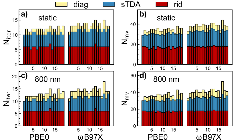
Figure 6: Performance of semiempirical preconditioning for computing static and dynamic (800 nm) dipole polarizabilities. The top row shows a) $N_{\text{iter}}$ and b) $N_{\text{mv}}$ for static polarizabilities, and the bottom row shows c) $N_{\text{iter}}$ and d) $N_{\text{mv}}$ for dynamic polarizabilities.

Similar to the excitation energy case, Fig. 6 shows that the rid preconditioner systematically improves over both the diagonal and the sTDA preconditioners, with similar behavior for both the static and dynamic polarizabilities. For PBE0, the rid preconditioner converges in 6.0 iterations on average, compared to 12.2 for the diagonal and 10.4 for the sTDA. This leads to speed ups of a factor of 2.0 and 1.2 for rid and sTDA, respectively. For $\omega$B97X, the rid preconditioner converges in 6.1 iterations on average, compared to 13.7 for the diagonal and 11.6 for the sTDA. This gives speed ups of a factor of 2.3 and 1.2 for rid and sTDA, respectively. Again, the rid preconditioner erases the difference in number of iterations needed between PBE0 and $\omega$B97X. We emphasize that the rid preconditioner fixes the disappointing performance of the sTDA preconditioner for the polarizability problem.

Table 2: The range and the average number of iterations, $N_{\text{iter}}$, required to converge static and dynamic (800 nm) polarizability calculations with the PBE0 and $\omega$B97X density functionals using diagonal, sTDA, and rid preconditioners.

		PBE0			$\omega$B97X
precond.		diag	sTDA	rid	diag	sTDA	rid
$N_{\text{iter}}$	min.	9	10	5	11	10	6
	max.	15	12	7	18	13	7
	avg.	12.2	10.4	6.0	13.7	11.6	6.1
$\zeta_{\text{iter}}$	min.	–	0.9	1.5	–	1.1	1.8
	max.	–	1.4	2.5	–	1.4	3.0
	avg.	–	1.2	2.0	–	1.2	2.3

5 Conclusions

TDDFT excitation energy and polarizability calculations are computationally expensive for large systems. Semiempirical models, like the TDDFT-ris model, are often designed to replace the need for ab initio calculations. However, we show that semiempirical models and ab initio models can be synergistically combined to accelerate ab initio calculations without any loss in accuracy.

We used the TDDFT-ris model as a starting point to systematically design a highly performant and broadly applicable preconditioner for calculations of excitation energies and polarizabilities within TDDFT. The final preconditioner, rid, uses an auxiliary basis with up to $d$ functions for the Coulomb terms and $s$ functions for the exchange terms, and a global scale factor of $\theta$=0.6. By construction, the rid preconditioner has virtually no additional cost compared to the ab initio matrix-vector products, and is applicable across the entire periodic table.

The rid preconditioner significantly outperforms both the diagonal and sTDA preconditioners for excitation energy and polarizability calculations. We find that the rid preconditioner converges in just 5-6 iterations on average for excitation energies and polarizabilities. In other words, the rid preconditioner speeds up excitation energy calculations by a factor of 2-5 compared to the diagonal preconditioner and speeds up polarizability calculations by a factor of 1.3-2.2. This makes the rid preconditioner the best performing preconditioner for TDDFT excitation energies and polarizabilities that we are aware of.

We emphasize two further points about the rid preconditioner. First, the rid preconditioner all but erases the difference in the number of iterations required to converge PBE0 compared to $\omega$B97X, indicating that it retains high performance across different density functionals. Second, the rid preconditioner successfully speeds up the polarizability calculations, thus fixing the disappointing performance of the sTDA preconditioner for the polarizability problem.

The excellent performance of the rid preconditioner may appear surprising in light of the common view that the Davidson algorithm can stagnate if the approximate matrix used in the preconditioner, $\mathbf{T}$, becomes “too close” to the exact matrix, $\mathbf{A}$.^{3, 23, 45} However, this “deficiency” in the Davidson algorithm turns out have little relevance to practical applications in quantum chemistry. As shown by Notay, when the Davidson algorithm is initiated with eigenvectors of $\mathbf{T}$—as we do here and as is common practice—then no stagnation occurs and both Davidson and Jacobi-Davidson provide similar convergence rates.²⁷ Our results support this conclusion, as we find no evidence at all of any deterioration in the performance of the Davidson algorithm when using increasingly accurate preconditioners.

Thus, the rid preconditioner is a general purpose preconditioner that can be used to accelerate the iterative calculation of TDDFT excitation energies and polarizabilities. In addition, because rid is fundamentally based on a transferrable approximation to the electron repulsion integrals, the same idea could be used to design preconditioners in other contexts. A rid-type preconditioner should be beneficial for any method where computing electron repulsion integrals are the bottleneck. We are especially eager to use the rid preconditioner in scenarios where the electronic Hessian are intensively called, such as non-adiabatic molecular dynamics, and excited state geometry optimization. We also envision the rid preconditioner proving invaluable when applied to vibrational frequency calculations, and in generating large datasets for machine learning models.

See the Supporting Information for definitions of the TUNE8 and PRECOND19 benchmark sets, results from tuning the number of initial guesses, the performance of the rid preconditioner for TDDFT eigenvalues, and the detailed set of results for all benchmark calculations.

This work was supported by a startup fund from Case Western Reserve University. This work made use of the High Performance Computing Resource in the Core Facility for Advanced Research Computing at Case Western Reserve University.

Data Availability

All code for this paper is available on Github under the MIT license.⁴⁶ The data supporting this study are openly available on the Open Science Framework under the Creative Commons license.⁴⁷

References

- Siegbahn 1977 Siegbahn, P. E. M. The Direct Configuration Interaction Method with a Contracted Configuration Expansion. Chem. Phys. 1977, 25, 197–205
- Knowles and Handy 1984 Knowles, P. J.; Handy, N. C. A New Determinant-Based Full Configuration Interaction Method. Chem. Phys. Lett. 1984, 111, 315–321
- Olsen et al. 1990 Olsen, J.; Jørgensen, P.; Simons, J. Passing the One-Billion Limit in Full Configuration-Interaction (FCI) Calculations. Chem. Phys. Lett. 1990, 169, 463–472
- Mitrushenkov 1994 Mitrushenkov, A. O. Passing the Several Billions Limit in FCI Calculations on a Mini-Computer. Chem. Phys. Lett. 1994, 217, 559–565
- Gao et al. 2024 Gao, H.; Imamura, S.; Kasagi, A.; Yoshida, E. Distributed Implementation of Full Configuration Interaction for One Trillion Determinants. J. Chem. Theory Comput. 2024, 20, 1185–1192
- Olsen and Jørgensen 1985 Olsen, J.; Jørgensen, P. Linear and Nonlinear Response Functions for an Exact State and for an MCSCF State. J. Chem. Phys. 1985, 82, 3235–3264
- Christiansen et al. 1998 Christiansen, O.; Jørgensen, P.; Hättig, C. Response Functions from Fourier Component Variational Perturbation Theory Applied to a Time-Averaged Quasienergy. Int. J. Quantum Chem. 1998,
- Parker and Furche 2018 Parker, S. M.; Furche, F. In Frontiers of Quantum Chemistry; Wójcik, M. J., Nakatsuji, H., Kirtman, B., Ozaki, Y., Eds.; Springer Singapore, 2018; pp 69–86
- Thouless 1960 Thouless, D. J. Stability Conditions and Nuclear Rotations in the Hartree-Fock Theory. Nuc. Phys. 1960, 21, 225–232
- Čížek and Paldus 1967 Čížek, J.; Paldus, J. Stability Conditions for the Solutions of the Hartree—Fock Equations for Atomic and Molecular Systems. Application to the Pi-Electron Model of Cyclic Polyenes. J. Chem. Phys. 1967, 47, 3976–3985
- Bauernschmitt and Ahlrichs 1996 Bauernschmitt, R.; Ahlrichs, R. Stability Analysis for Solutions of the Closed Shell Kohn–Sham Equation. J. Chem. Phys. 1996, 104, 9047
- Davidson 1975 Davidson, E. R. The Iterative Calculation of a Few of the Lowest Eigenvalues and Corresponding Eigenvectors of Large Real-Symmetric Matrices. J. Comput. Phys. 1975, 17, 87–94
- Weiss et al. 1993 Weiss, H.; Ahlrichs, R.; Häser, M. A Direct Algorithm for Self-consistent-field Linear Response Theory and Application to C60: Excitation Energies, Oscillator Strengths, and Frequency-dependent Polarizabilities. J. Chem. Phys. 1993, 99, 1262–1270
- Furche et al. 2016 Furche, F.; Krull, B. T.; Nguyen, B. D.; Kwon, J. Accelerating Molecular Property Calculations with Nonorthonormal Krylov Space Methods. J. Chem. Phys. 2016, 144, 174105
- Parrish et al. 2016 Parrish, R. M.; Hohenstein, E. G.; Martínez, T. J. “Balancing” the Block Davidson–Liu Algorithm. J. Chem. Theory Comput. 2016, 12, 3003–3007
- Bauernschmitt et al. 1997 Bauernschmitt, R.; Häser, M.; Treutler, O.; Ahlrichs, R. Calculation of Excitation Energies within Time-Dependent Density Functional Theory Using Auxiliary Basis Set Expansions. Chem. Phys. Lett. 1997, 264, 573–578
- Hu et al. 2020 Hu, W.; Liu, J.; Li, Y.; Ding, Z.; Yang, C.; Yang, J. Accelerating Excitation Energy Computation in Molecules and Solids within Linear-Response Time-Dependent Density Functional Theory via Interpolative Separable Density Fitting Decomposition. J. Chem. Theory Comput. 2020, 16, 964–973
- Ufimtsev and Martínez 2008 Ufimtsev, I. S.; Martínez, T. J. Quantum Chemistry on Graphical Processing Units. 1. Strategies for Two-Electron Integral Evaluation. J. Chem. Theory Comput. 2008, 4, 222–231
- Isborn et al. 2011 Isborn, C. M.; Luehr, N.; Ufimtsev, I. S.; Martínez, T. J. Excited-State Electronic Structure with Configuration Interaction Singles and Tamm–Dancoff Time-Dependent Density Functional Theory on Graphical Processing Units. J. Chem. Theory Comput. 2011, 7, 1814–1823
- Zhou and Parker 2021 Zhou, Z.; Parker, S. M. Accelerating molecular property calculations with semiempirical preconditioning. J. Chem. Phys. 2021, 155, 204111
- Grimme 2013 Grimme, S. A Simplified Tamm-Dancoff Density Functional Approach for the Electronic Excitation Spectra of Very Large Molecules. J. Chem. Phys. 2013, 138, 244104
- Zhou et al. 2023 Zhou, Z.; Della Sala, F.; Parker, S. M. Minimal Auxiliary Basis Set Approach for the Electronic Excitation Spectra of Organic Molecules. J. Phys. Chem. Lett. 2023, 1968–1976
- Sleijpen and Van der Vorst 1996 Sleijpen, G. L.; Van der Vorst, H. A. A Jacobi–Davidson Iteration Method for Linear Eigenvalue Problems. SIAM Journal on Matrix Analysis and Applications 1996, 17, 401–425
- Hochstenbach and Notay 2006 Hochstenbach, M.; Notay, Y. The Jacobi–Davidson Method. GAMM-Mitteilungen 2006, 29, 368–382
- Van Dam et al. 1996 Van Dam, H.; Van Lenthe, J.; Sleijpen, G.; Van Der Vorst, H. An Improvement of Davidson’s Iteration Method: Applications to MRCI and MRCEPA Calculations. J. Comp. Chem. 1996, 17, 267–272
- Rappoport et al. 2023 Rappoport, D.; Bekoe, S.; Mohanam, L. N.; Le, S.; George, N.; Shen, Z.; Furche, F. Libkrylov: A Modular Open-Source Software Library for Extremely Large on-the-Fly Matrix Computations. J. Comp. Chem. 2023, 44, 1105–1118
- Notay 2004 Notay, Y. Is Jacobi–Davidson Faster than Davidson? SIAM Journal on Matrix Analysis and Applications 2004, 26, 522–543
- Bannwarth and Grimme 2014 Bannwarth, C.; Grimme, S. A Simplified Time-Dependent Density Functional Theory Approach for Electronic Ultraviolet and Circular Dichroism Spectra of Very Large Molecules. Comput. Theor. Chem. 2014, 1040-1041, 45–53
- Asadi-Aghbolaghi et al. 2020 Asadi-Aghbolaghi, N.; Rüger, R.; Jamshidi, Z.; Visscher, L. TD-DFT+TB: An Efficient and Fast Approach for Quantum Plasmonic Excitations. J. Phys. Chem. C 2020, 124, 7946–7955
- Giannone and Della Sala 2020 Giannone, G.; Della Sala, F. Minimal auxiliary basis set for time-dependent density functional theory and comparison with tight-binding approximations: Application to silver nanoparticles. J. Chem. Phys. 2020, 153, 084110
- Baerends et al. 1973 Baerends, E.; Ellis, D.; Ros, P. Self-consistent molecular Hartree—Fock—Slater calculations I. The computational procedure. Chem. Phys. 1973, 2, 41
- Dunlap et al. 1979 Dunlap, B. I.; Connolly, J. W. D.; Sabin, J. R. On Some Approximations in Applications of X Theory. J. Chem. Phys. 1979, 71, 3396–3402
- Eichkorn et al. 1995 Eichkorn, K.; Treutler, O.; Öhm, H.; Häser, M.; Ahlrichs, R. Auxiliary basis sets to approximate Coulomb potentials. Chem. Phys. Lett. 1995, 240, 283
- Heinze et al. 2000 Heinze, H. H.; Görling, A.; Rösch, N. An efficient method for calculating molecular excitation energies by time-dependent density-functional theory. J. Chem. Phys. 2000, 113, 2088
- Neese and Olbrich 2002 Neese, F.; Olbrich, G. Efficient use of the resolution of the identity approximation in time-dependent density functional calculations with hybrid density functionals. Chem. Phys. Lett. 2002, 362, 170–178
- Pedersen et al. 2009 Pedersen, T.; Aquilante, F.; Lindh, R. Density fitting with auxiliary basis sets from Cholesky decompositions. Theor. Chem. Acc. 2009, 124, 1
- Weigend et al. 2009 Weigend, F.; Kattannek, M.; Ahlrichs, R. Approximated electron repulsion integrals: Cholesky decomposition versus resolution of the identity methods. J. Chem. Phys. 2009, 130, 164106
- Stoychev et al. 2017 Stoychev, G. L.; Auer, A. A.; Neese, F. Automatic generation of auxiliary basis sets. J. Chem. Theory Comput. 2017, 13, 554
- Ghosh et al. 2008 Ghosh, D. C.; Biswas, R.; Chakraborty, T.; Islam, N.; Rajak, S. K. The wave mechanical evaluation of the absolute radii of atoms. Journal of Molecular Structure: THEOCHEM 2008, 865, 60–67
- Risthaus et al. 2014 Risthaus, T.; Hansen, A.; Grimme, S. Excited States Using the Simplified Tamm–Dancoff-Approach for Range-Separated Hybrid Density Functionals: Development and Application. Phys. Chem. Chem. Phys. 2014, 16, 14408–14419
- Sun et al. 2018 Sun, Q.; Berkelbach, T. C.; Blunt, N. S.; Booth, G. H.; Guo, S.; Li, Z.; Liu, J.; McClain, J. D.; Sayfutyarova, E. R.; Sharma, S.; Wouters, S.; Chan, G. K.-L. PySCF: The Python-Based Simulations of Chemistry Framework. WIREs Comput. Mol. Sci. 2018, 8, e1340
- Perdew et al. 1996 Perdew, J. P.; Ernzerhof, M.; Burke, K. Rationale for Mixing Exact Exchange with Density Functional Approximations. J. Chem. Phys. 1996, 105, 9982–9985
- Weigend and Ahlrichs 2005 Weigend, F.; Ahlrichs, R. Balanced Basis Sets of Split Valence, Triple Zeta Valence and Quadruple Zeta Valence Quality for H to Rn: Design and Assessment of Accuracy. Phys. Chem. Chem. Phys. 2005, 7, 3297–3305
- Chai and Head-Gordon 2008 Chai, J.-D.; Head-Gordon, M. Systematic Optimization of Long-Range Corrected Hybrid Density Functionals. J. Chem. Phys. 2008, 128, 084106
- Windom and Bartlett 2023 Windom, Z. W.; Bartlett, R. J. On the Iterative Diagonalization of Matrices in Quantum Chemistry: Reconciling Preconditioner Design with Brillouin–Wigner Perturbation Theory. J. Chem. Phys. 2023, 158, 134107
- 46 Minimal auxiliary basis preconditioned Davidson implementation available at github.com/John-zzh/Davidson
- Zhou and Parker 2023 Zhou, Z.; Parker, S. M. Minimal auxiliary basis set approach for the electronic excitation spectra of organic molecules; DOI: 10.17605/OSF.IO/X5BSV. 2023; osf.io/x5bsv