Improving flux ratio anomaly precision by measuring gravitational lens multipole moments with extended arcs

Abstract

In a strong gravitational lens, perturbations by low-mass dark matter halos can be detected by differences between the measured image fluxes relative to the expectation from a smooth model for the mass distribution which contains only the gravitational effects of the main deflector. The abundance of these low-mass structures can be used to constrain the properties of dark matter. Traditionally only the lensed quasar positions have been to predict the smooth-model flux ratios. We demonstrate that significant additional information can be gained by using the lensed quasar host galaxy which appears as an extended arc and constrains the smooth-model over a much larger angular area. We simulate Hubble Space Telescope-quality mock observations based on the lensing system WGD2038-4008 and we compare the model-predicted flux ratio precision and accuracy for two cases; one of which the inference is based only on the lensed quasar image positions, and the other based on the extended arcs as well as lensed quasar image positions. For our mock lens systems we include both elliptical, and higher order $m=3$ and $m=4$ multipole terms in the smooth-mass distributions with amplitudes based on the optically measured shapes of massive elliptical galaxies. We find that the extended arcs improve the precision of the model-predicted flux ratios by a factor of 6-8, depending on the strength of the multipole terms. Furthermore, with the extended arcs, we are also able to accurately recover the $m=3,4$ mass multipole strengths and angles $a_{3}\!/\!a$, $a_{4}\!/\!a$, $\phi_{3}-\phi_{0}$, and $\phi_{4}-\phi_{0}$ to a precision of 0.002, 0.002, $3^{\circ}$ and $3^{\circ}$, respectively. This work implies that lensed arcs can constrain deviations from ellipticity in strong lens systems, and potentially lead to more robust constraints on substructure properties from flux ratios.

1 Introduction

Dark matter is the major matter component of the Universe [1]. Despite extensive efforts to directly detect dark matter particles, there has been no confirmed detection. As a result, the detailed properties of dark matter are still in the realm of theoretical modeling and conjecture.

Gravity is the only known observable tracer of dark matter. Thus, gravitational lensing, a phenomenon where light path is bent along the warped spacetime due to gravity, serves as a unique probe of the dark matter mass distribution. This methodology is considered unique because it does not require to observe baryonic components (such as stars and gas) within dark matter halos.

Different dark matter models predict different abundances and mass profiles of low-mass dark matter halos, and gravitationally lensed images can be used to distinguish between a variety of dark matter models [see 2, and references therein].

Flux ratio anomalies of gravitationally lensed quasars are the disparity between the observed flux ratios of lensed images and the flux ratios expected from a smooth mass distribution which represents the large-scale distribution of lensing galaxy’s mass (a.k.a. “macromodel”). The smooth, large-scale mass distribution is primarily responsible for causing multiple images of the background source to appear and determining their positions. Low-mass dark matter halos within the lensing galaxy and along the line of sight (a.k.a. “substructures”) make relatively little impact to the image positions relative to measurement uncertainties, but can introduce perturbations to the lensed image magnifications relative to the smooth-mass distribution alone, which results in ‘flux-ratio anomalies’ [see 3, 4, 5, 2, and references therein]. Such anomalies demonstrate the existence of low-mass substructures and have been used to infer population level statistics of their mass function and mass distribution [6, 7, 8].

Because the flux ratio anomaly method depends on the flux measurements relative to smooth-model’s prediction, accurate representation of the smooth model is essential for the inference of dark matter characteristics. Traditionally, only the lensed point source positions have been used to constrain the smooth-mass distribution. This yields large uncertainties of order 10-50% in the underlying smooth-model flux ratios which are comparable to or larger than the measurement uncertainties of the actual flux ratios themselves [see, e.g. 9]. Existing measurements of lens flux ratios from HST reach, on average, 6% precision [9], while mid-IR flux ratios measured with JWST can reach precisions of 1% [10]. Improving the precision of the smooth-model flux ratio predictions would therefore make a significant impact on the constraining power of gravitational lenses.

While many past flux ratio anomaly studies modelled the smooth-mass distribution as an elliptical mass profile with external shear, recent studies have begun investigating the potential impact from lens mass distribution that deviates from a perfect elliptical shape [e.g. 11]. Multipoles describe higher order perturbations to the mass distribution that cannot be captured by an elliptical profile [12, 13, 14, 15, 5, 16, 17, 18]. Of particular interest are multipoles of order $m\!=\!3$ and $m\!=\!4$ as these are prominent deviations from ellipticity observed in the light distribution of field elliptical galaxies [19].

Existing constraints on dark matter from [20, 21, 22, 23] include an $m=4$ multipole term, which adds boxyness and diskyness to the main deflector mass profile. The amplitude of this mass component is constrained by image positions and flux ratios jointly with the substructure properties. A recent simulation work [24] presented the dark matter analysis pipeline with both $m=3$ and $m=4$ multipoles. Warm dark matter constraint using the JWST data is also given in [25].

In this work, we explore how the flux ratios of a gravitational lens are affected by multipoles in the absence of substructure, and secondly, how much the precision and accuracy of smooth-model-predicted flux ratios can be improved by including the lensed quasar host galaxy (“extended arcs”, or simply “arcs” hereafter). As the arcs wraps around the main deflector, it provides constraints on the mass profile of the main deflector over larger angular scales than the quasar image positions and their flux ratios [26, 27]. This work is a complement to the work presented in [24], which included multipoles, imaging data with lensed arcs, and low mass dark matter substructures in their analysis. Note that, in this work, we do not assume dark matter substructures in the system such that the impact of multipoles and lensed arcs can be clearly demonstrated without complications from substructures.

The structure of this paper is as follows: In Section 2 we describe how we model the quadruply imaged quasar lens. In Section 3 we discuss priors of multipoles based on the optical multipole measurements. Section 4 addresses the simulated observation and inference processes. Section 5 explains the inference process and the measurement of parameters. Section 6 outlines the inference result and in Section 7 we discuss the results and conclusions. lenstronomy [28, 29] is used for lens modeling and fitting processes.

2 Quadruply lensed quasar modeling

Our goal is to determine how accurately and precisely we can recover the smooth model predicted flux ratios under various assumptions about the available data, and the modelling choices. We do this by generating mock data sets with varying properties. Here we describe the model components used to simulate, and to infer the properties of the quasar lenses.

2.1 Light components

There are three light components included in the light model as described below. Table 5 gives specific parameter values for these model components.

Quasar The lensed quasar images are modeled as point sources because the angular scales of target quasars are micro-arcseconds and thus unresolved by optical telescopes. The quasar point sources are present in all mock images.

Source light This is the surface brightness model of the host galaxy of the quasar. The extended arcs come from the lensing of the extended quasar host galaxy. When present, we model this component as an elliptical Sérsic profile [30].

Lens light The surface brightness model of the lens galaxy. We model this as an elliptical Sérsic profile. This is present in all mock images.

2.2 Smooth-mass components

There are two components included in the smooth-mass model as follows. The mass model parameters used to generate the mock data are given in Tables 1 and 4. Note that dark matter substructures are not included in this work to clearly demonstrate the impact of multipoles and lensed arcs without substructure lensing.

Multipole Scenario	Parameter Name	Simulation Truth	Fitting Prior
No Multipoles	$a_{3}/a$	$0$	$\mathcal{N}(0,0.006)$
	$\phi_{3}-\phi_{0}$	$0$	$U(-\pi/6,\pi/6)$
	$a_{4}/a$	$0$	$\mathcal{N}(0.005,0.013)$
	$\phi_{4}-\phi_{0}$	$0$	Fixed to $0$
Mild & Aligned $m=4$	$a_{3}\!/\!a$	$-0.006$	$\mathcal{N}(0,0.006)$
	$\phi_{3}-\phi_{0}$	$-0.05$ ($-3.0^{\circ}$)	$U(-\pi/6,\pi/6)$
	$a_{4}/a$	$0.01$	$\mathcal{N}(0.005,0.013)$
	$\phi_{4}-\phi_{0}$	$0$	Fixed to $0$
Strong & Aligned $m=4$	$a_{3}\!/\!a$	$-0.006$	$\mathcal{N}(0,0.006)$
	$\phi_{3}-\phi_{0}$	$-0.05$ ($-3.0^{\circ}$)	$U(-\pi/6,\pi/6)$
	$a_{4}/a$	$0.03$	$\mathcal{N}(0.005,0.013)$
	$\phi_{4}-\phi_{0}$	$0$	Fixed to $0$
Mild & Misaligned $m=4$	$a_{3}\!/\!a$	$-0.006$	$\mathcal{N}(0,0.006)$
	$\phi_{3}-\phi_{0}$	$-0.05$ ($-3.0^{\circ}$)	$U(-\pi/6,\pi/6)$
	$a_{4}/a$	0.01	$\mathcal{N}(0.005,0.013)$
	$\phi_{4}-\phi_{0}$	$0.17\ (10^{\circ})$	$U(-\pi/8,\pi/8)$

Table 1: $m\!=\!3,4$ multipole parameters with four different scenarios. The priors of $a_{3}\!/\!a$ and $a_{4}\!/\!a$ are set using the distribution shown in Figure 3.

Base mass model For all mock lenses, and inferences, we use an underlying Elliptical Power Law (EPL) mass profile [31]. We also include external shear which can be caused by external sources such as galaxy clusters or large-scale structure [32, 33, 34].

Multipole mass profiles Multipole mass profiles add azimuthal perturbation to the mass profile of the lens, on top of the elliptical profile. In order to test our results under different mass multipoles, we vary multipole parameters as described in Table 1. Note that there are different conventions on how to define multipoles and we follow the convention of [35, 36, 18]. In Appendix B we provide relations between this and other commonly used conventions.

When an order-$m$ multipole is added to an elliptical profile, the isodensity (i.e. constant convergence $\kappa$) contours are deformed from a purely elliptical isodensity contours. The deviation of the new isodensity contour from the ellipse can be expressed with a cosine function $\delta\theta=a_{m}\cos(m(\phi-\phi_{m}))$, where $\phi_{m}$ is the angle of the multipole profile’s orientation. Note that the deviation amplitude $a_{m}$ depends on which contour is chosen. When geometric similarity is assumed between the contours on different scales, the radial deviation is proportional to the size of the ellipse; i.e. $a_{m}\propto a$, where $a$ is the semi-major axis of the ellipse and satisfies $a=\frac{1}{2\kappa}{\theta_{E}}/\!{\sqrt{q}}$. The ratio $a_{m}\!/\!a$ is the key parameter that determines the shape of the deformed isodensity contour.

Choosing the standard isodensity contour with $\kappa\!=\!\frac{1}{2}$ gives the semi-major axis of the ellipse as the effective Einstein radius $a\mbox{\footnotesize$(\kappa\!=\!\frac{1}{2})$ }=\theta_{E}/\!\sqrt{q}$. The deviation amplitude there, $a_{m}\mbox{\footnotesize$(\kappa\!=\!\frac{1}{2})$}$ , is used for setting the deflection potential. The deviation of the isodensity contours from the standard ellipse with $\kappa\!=\!\frac{1}{2}$ is

$$\delta\theta\rvert_{\kappa=\frac{1}{2}}=a_{m}\mbox{\footnotesize$(\kappa\!=\!\frac{1}{2})$}\ \cos(m(\phi-\phi_{m})).$$ (2.1)

We let $a_{m}\mbox{\footnotesize$(\kappa\!=\!\frac{1}{2})$}$ be either positive or negative, and $\phi_{m}$ be limited to $(-\frac{\pi}{2m},\frac{\pi}{2m}]$ to avoid angular multiplicity (see Appendix B). The multipole deflection potential that satisfies the desired radial deviation is as follows (see [15, 36]) .

$$\psi_{m}(\theta)=\theta\ \frac{a_{m}\mbox{\footnotesize$(\kappa\!=\!\frac{1}{2})$}}{1-m^{2}}\cos(m(\phi-\phi_{m}))$$ (2.2)

Note that, with a given value of $a_{m}\!/\!a$, the $a_{m}\scriptstyle(\kappa=\frac{1}{2})$ value is calculated by

$$a_{m}\mbox{\footnotesize$(\kappa\!=\!\frac{1}{2})$}=a_{m}\!/\!a\ a\mbox{\mbox{\footnotesize$(\kappa\!=\!\frac{1}{2})$}}=\ a_{m}\!/\!a\ \frac{\theta_{E}}{\sqrt{q}}.$$ (2.3)

Thus, the deflection potential can be set up based on either $a_{m}\!/\!a$ or $a_{m}\mbox{\footnotesize$(\kappa\!=\!\frac{1}{2})$}$. In this paper, we stick to $a_{m}\!/\!a$ convention.

We included $m\!=\!3$ (hexapole) and $m\!=\!4$ (octapole) multipoles in both the simulation and inference. The $m\!=\!3$ and $m\!=\!4$ multipoles measure the triangle-like and quadrangle-like deformation on the isodensity contour, respectively. They are paramaterized with their multipole strength $a_{m}\!/\!a$ and their angle relative to the elliptical profile $\phi_{m}-\phi_{0}$, where $\phi_{0}$ refers to the angle of the elliptical profile (see Figure 1). In Section 3 we explain how we select values for the multipole parameters.

The $m\!=\!4$ multipole is also known as boxy/diskyness, because it makes an elliptical profile either boxy (a.k.a. peanut-shaped) or disky. When the orientation of the multipole profile and the elliptical profile are well aligned (i.e. $\phi_{m}\approx\phi_{0}$, where $\phi_{0}$ is the angle of the elliptical profile), $a_{4}\!/\!a>0$ results in a disky profile and $a_{4}\!/\!a<0$ a boxy profile. Meanwhile, the sign of $a_{3}\!/\!a$ does not change the overall shape but the orientation (see Figure 2).

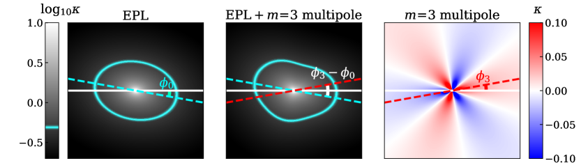
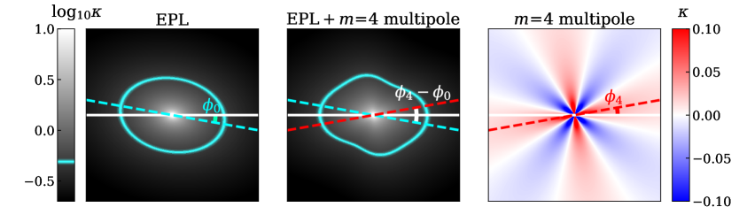
Figure 1: Impact of misaligned ($\phi_{m}\!\neq\!\phi_{0}$) $m\!=\!3$ (upper) and $m\!=\!4$ (lower) multipole profile on the convergence with the angular conventions $\phi_{0}$ and $\phi_{m}$. The isodensity curve is shown in cyan. (Left) Convergence of EPL-only lens mass model with $\phi_{0}=-0.175\ (-10^{\circ})$. (Middle) Convergence of EPL+multipole. (Right) Convergence of $m\!=\!3$ and $m\!=\!4$ multipole with $a_{m}\!/\!a=0.05$ and $\phi_{m}=0.175\ (10^{\circ})$. For better visualization, $|a_{m}/a|$ is set to be larger than expected in typical systems.

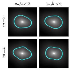
Figure 2: Impact of aligned ($\phi_{m}\!=\!\phi_{0}$) $m\!=\!3$ (upper) and $m\!=\!4$ (lower) multipole profile on the convergence with different signs of $a_{m}\!/\!a$. (Left) Convergence of EPL+multipole with $a_{m}\!/\!a=+0.05$. (Right) Convergence of EPL+multipole with $a_{m}\!/\!a=-0.05$. For better visualization, $|a_{m}\!/\!a|$ is set to be larger than expected in typical systems.

2.3 Data quality

We create mock observations based on Hubble Space Telescope’s WFC3 imaging data from programs GO-15320 and GO-15652, which carried out a uniform multi-band imaging campaign of 31 quadruply imaged quasars. We base our simulations on the observations with F814W which had the best combination of sensitivity and PSF width.

The exposure time is set to be 920 seconds, the pixel size is set to be $0.04$ arcseconds, and the background noise level is set to be $0.006$ photons/second for each pixel. We modeled the point spread function (PSF) as a two dimensional Gaussian with full-width-half-max of 0$.\!\!^{\prime\prime}$1. Note that this choice of PSF is a simplification; in real observational data, the PSF is more complicated than a Gaussian and needs to be inferred from the data.

3 Multipole parameter values

In this section we explore what reasonable priors are for the multipole parameters of the mass distribution. The multipole parameters of the lens mass profiles have not been well constrained from the observation so far. However, surveys of the optical profiles of elliptical galaxies can be used as a reference and may provide an upper limit on the expected multipole amplitudes. The optical $a_{m}$ and $a$ are defined the same way as the mass profile’s isodensity contours, but instead using isophote contours. The ratio of deformation amplitude and the semi-major axis, $a_{m}\!/\!a$, has been measured with different galaxies and different radii [37, 19, 38, 39]

It has been shown that $m=4$ multipole amplitude is larger than $m=3$ multipole amplitude, and that the $m=4$ multipole tends to align with the axis of the ellipse [19]. See Figure 3 for the distribution of $a_{3}\!/\!a$ and $a_{4}\!/\!a$ measured from the isophotes of 823 E/S0 galaxies, of which the original data is provided by [19]. We selected a subset of galaxies with $q>1/2$. This is to ensure that the galaxies are representative of strong gravitational lenses which are used to infer the properties of dark matter [9]. The original number of galaxies is 847, and the selection removed 24 of them. The marginal distributions are calculated with a weighting of ${v_{dis}}^{4}$; see the bottom left of Figure 3 for the velocity dispersion distribution .

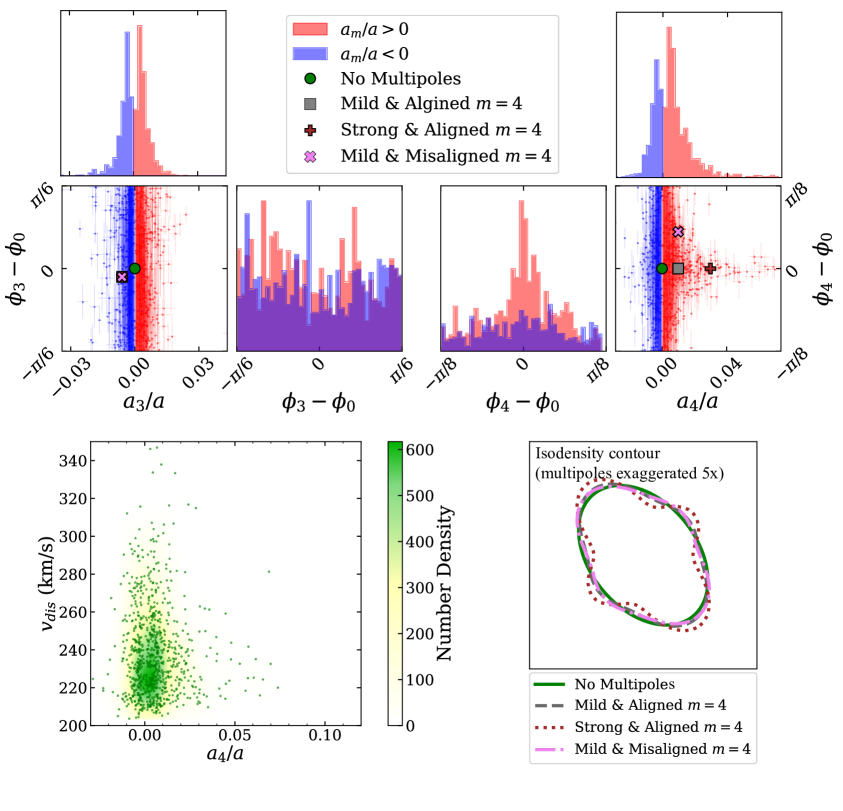
Figure 3: (Upper half) The optical multipole amplitude ($a_{m}\!/\!a$) and the multipole-ellipse misalignment angle ($\phi_{m}-\phi_{0}$) for $m=3,\ 4$ of 823 elliptical (E) and lenticular (S0) galaxies, together with each data point’s uncertainty. The original data is from the isophote curve survey [19]. Samples with $a_{m}\!/\!a>0$ and $a_{m}\!/\!a<0$ are plotted separately with red and blue, respectively. Note that multipole profiles with positive $a_{4}\!/\!a$ (diskyness) tend to align with the elliptical profile ($\phi_{4}\approx\phi_{0}$), and this tendency is stronger when $a_{4}\!/\!a$ is greater. Data points are weighted by 4-th power of velocity distribution, ${v_{dis}}^{4}$. (Bottom left) The optical $m=4$ multipole amplitude ($a4\!/\!a$) and velocity dispersion ($v_{dis}$) of the samples. (Bottom right) The isodensity contour of four multipole scenarios, where the multipole amplitude is exaggerated by five times for noticeable visualization. Green circles and solid line, gray squares and dashed line, crimson pluses and dotted line, and pink cross and dash-dotted line correspond to ‘No Multipole’, ‘Mild & Aligned $m=4$’, ‘Strong & Aligned $m=4$’, and ‘Mild & Misaligned $m=4$’ scenarios, respectively. For $m\!=\!3$ multipole, all scenarios except ‘No Multipoles’ assume the same strength and orientation. For $m\!=\!4$ multipole, the strength and orientation values are varied. Refer to Table 1 for exact multipole values of the scenarios.

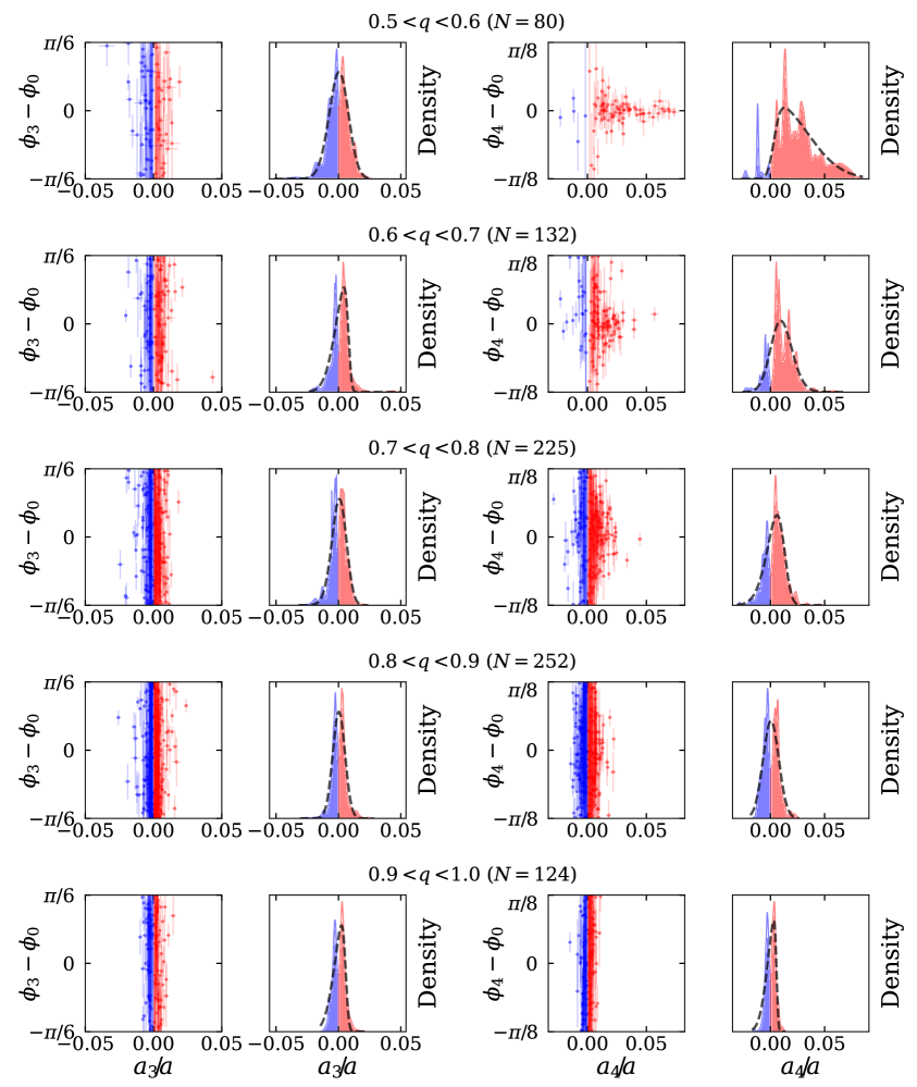
Figure 4: The distribution of the optical $a_{m}\!/\!a$ and $\phi_{m}-\phi_{0}$ and the marginal density distribution of $a_{m}\!/\!a$ with gray dashed lines being skewed normal distribution fit for different range of the axis ratio $q$ for $m=3$ (left) and $m=4$ (right). The marginal density distribution is plotted and fitted after smoothing with each data point’s uncertainty. From the top to the bottom, the range of $q$ changes from $(0.5,0.6)$ to $(0.9,1.0)$ incrementally, as noted in the figure. The skewed normal distribution fit parameters are shown in Table 2. The original data is from the isophote curve survey by [19]. Data points are weighted by 4-th power of velocity distribution.

Plotting the amplitude ratio $a_{m}\!/\!a$ together with the angle misalignment between the optical multipole with the optical ellipse $\phi_{m}-\phi_{0}$ shows an important correlation; the misalignment is small for $a_{4}\!/\!a>0$ only, and the greater $a_{4}\!/\!a$ is, the smaller the misalignment (see Figure 3). In other words, the ‘diskyness’ tends to align with the ellipse, whereas the ‘boxyness’ and $m=3$ multipoles do not. We use these trends when selecting parameters for our simulated lenses as described in Section 4.

Figure 4 shows the distribution of $a_{m}\!/\!a$ and $\phi_{m}-\phi_{0}$ in different ranges of axis ratio $q$. It is notable that highly disky galaxies (e.g. $a_{4}\!/\!a>0.03$) are likely to be highly elliptical galaxies (e.g. $q<0.7$). In other words, if a lensing galaxy has a high ellipticity, its $a_{4}\!/\!a$ prior should be assumed broader. Table 2 provides the best-fit skewed normal distribution parameters for $a_{m}\!/\!a$ for different ranges of $q$.

	$a_{3}\!/\!a$ best fit			$a_{4}\!/\!a$ best fit
	$\alpha$	$\xi$	$\omega$	$\alpha$	$\xi$	$\omega$
$0.5<q<0.6$	$-0.9061$	$0.0050$	$0.0093$	$6.5002$	$0.0031$	$0.0307$
$0.6<q<0.7$	$-4.7989$	$0.0080$	$0.0096$	$1.1810$	$0.0028$	$0.0127$
$0.7<q<0.8$	$-1.1501$	$0.0047$	$0.0074$	$-2.3081$	$0.0125$	$0.0127$
$0.8<q<0.9$	$-0.4360$	$0.0020$	$0.0052$	$-0.1258$	$0.0011$	$0.0074$
$0.9<q<1.0$	$-4.1022$	$0.0058$	$0.0082$	$-5.8448$	$0.0056$	$0.0078$

Table 2: Skewed normal distribution best-fit parameters for $a_{m}\!/\!a$ for $m=3$ and $m=4$. Here, $\alpha$ is the skeweness parameter and represents how skewed the distribution is. $\xi$ is the location parameter and denotes where the peak is. $\omega$ is the scale parameter and indicates how wide the distribution is.

4 Mock observation

To simulate a realistic HST-quality image of quads, we chose a reference quad system WGD2038-4008 because it has clear extended arcs [41]. This system has a source redshift of $z_{\text{source}}=0.777$, $z_{\text{lens}}=0.230$ [42, 43]. We selected the model parameters for our mock observations by fitting the original HST F814W image of this system with our model including the lensed quasar point sources and host galaxy as well as the base mass model. This ensures that in addition to realistic signal to noise, our mock lenses will have typical properties of gravitational lenses including potential contamination from the deflector light and realistic extended quasar host galaxy brightness. The values of the light model parameters are given in Table 5, and the base mass parameters values are given in Table 4.

We also include higher order multipole perturbations in our mass models, as described in Section 2. We base our parameter choices on the observations of Hao et al. [19] of elliptical galaxy isophotes, as described in Section 3. This choice implicitly assumes that the shape of the light profile would trace the shape of the underlying projected mass profile. However, the dark matter distribution is thought to be purely elliptical and thus most of the multipole component would be from the baryonic mass. For that reason, we expect that the absolute value of the amplitude of the multipole mass term $|a_{m}\!/\!a|$ will be smaller than that observed in the light. Thus, the light multipole absolute amplitudes provide the upper bounds for the mass multipole absolute amplitudes.

We consider four scenarios for the multipoles of the main deflector as described in Table 1. The multipole parameters of each scenario are marked on Figure 3 compared to the optical survey from [19]. The first scenario, ‘No Multipoles’ has $a_{3}\!/\!a=0,\ a_{4}\!/\!a=0$. The other three scenarios have $m=3$ and $m=4$ multipoles. The $m=3$ multipoles are set to be the same for all three scenarios ($a_{3}\!/\!a=-0.006$, $\phi_{3}-\phi_{0}=-0.05$), whereas the $m=4$ multipole settings differ. They are named ‘Mild & Aligned $m=4$’, ‘Strong & Aligned $m=4$’, and ‘Mild & Misaligned $m=4$’. ‘Mild’ and ‘Strong’ correspond to the multipole amplitude of $a_{4}\!/\!a=0.01$ and $a_{4}\!/\!a=0.03$, respectively. ‘Aligned’ and ‘Misaligned’ correspond to $\phi_{4}-\phi_{0}=0$ and $\phi_{4}-\phi_{0}=0.17\ (10^{\circ})$. Note that there is no ‘Strong & Misaligned $m=4$’ scenario because such a configuration is not common, as Figure 3 and 4 show.

These multipole scenarios are selected as they are representative of realistic combinations of parameter values seen in galaxy isophotes, and they span a possible range of perturbations to the lens models. Considering the axis ratio of the lensing galaxy $q=0.58$, these $a_{4}\!/\!a$ values are reasonable test cases based on the optical multipole survey, as shown in Figure 4 and Table 2.

For each multipole scenario described above, we made two simulated observations of the lens system; one in which only point sources were detected, and the other with point sources and arcs. The mock observation data was generated using lenstronomy. Figure 5 gives an example of two of our mock data sets. Note that the change from one multipole scenario to another is quite subtle (e.g. slight shift of point sources and arcs), and thus not displayed here.

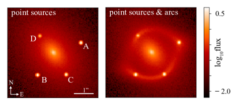
Figure 5: Comparison of simulations of HST-quality quadruply imaged quasars with point sources only (left) and point sources and extended arcs (right). The four quasar images are marked as A, B, C, and D. Note that the ‘point sources only’ case uses limited information (point source positions) only, whereas the ‘point sources and extended arcs’ case corresponds to an analysis using complete information with extended arcs. This way we can measure how much of improvement comes when the full observation with extended arcs is modeled, compared to using images positions only.

5 Inference and measurements

5.1 Model scenarios

For each simulated observation described in Section 4, we set up the lens modeling priors as described in Table 1, 4 and 5. For the three scenarios ‘No Multipoles’, ‘Mild and Aligned $m=4$’, and ‘Strong and Aligned $m=4$’ we keep $\phi_{4}=0$ fixed in the modelling. For the case ‘Mild and Misaligned $m=4$’ we allow $\phi_{4}-\phi_{0}$ to vary during the modelling. Other parameter priors are kept the same.

5.2 Inference

For each simulated observation with different multipole scenarios, we perform the inference. The lensed quasar image fluxes are not used as a constraint in the model because at the wavelengths of HST optical broad-band imaging the flux is dominated by emission from the quasar accretion disk which is contaminated by stellar microlensing. To avoid this potential source of contamination, for each proposed set of model parameters, we use a linear inversion to solve for the value of the point source image fluxes that provides the best fit to the imaging data and do not use the fluxes to constrain the lens model (i.e. we do not compare the model fluxes with the true fluxes in the fitting process), as done by other studies of lensed quasars using HST [e.g. 27, 42]. To clarify, the purpose of this scheme is not to fit the lens model using all available data but to understand the maximum improvement on the smooth mass model and its predicted flux ratios from additional arc information. Thus, flux ratios are not used to constrain the lens model.

We then infer the lens model parameters from the mock data following the standard lenstronomy fitting procedure [28, 29]. We begin with particle swarm optimization (PSO) to find an approximate solution that maximizes the likelihood of the model followed by Markov Chain Monte Carlo (MCMC) sampling to estimate the probabilistic distribution of parameters based on a Bayesian approach. After each MCMC sampling chain converges, the initial samples before convergence are discarded (burn-in). From the remaining part of the chain, 500,000 samples were randomly drawn and used to evaluate the probabilistic distribution of the sampled parameters as well as the model-predicted flux ratios.

The model-predicted flux ratios of each MCMC sample were calculated by the ratio of magnification values at the lensed quasar points, where the magnification at a given point is given as

$$\mu(\vec{\theta})=\frac{1}{(1-\kappa)^{2}-({\gamma_{1}}^{2}+{\gamma_{2}}^{2})},$$ (5.1)

where $\kappa=\frac{1}{2}\left[\frac{\partial^{2}\psi}{\partial{\theta_{1}}^{2}}+\frac{\partial^{2}\psi}{\partial{\theta_{2}}^{2}}\right]$, $\gamma_{1}=\frac{1}{2}\left[\frac{\partial^{2}\psi}{\partial{\theta_{1}}^{2}}-\frac{\partial^{2}\psi}{\partial{\theta_{2}}^{2}}\right]$, and $\gamma_{2}=\frac{\partial^{2}\psi}{\partial{\theta_{1}}\partial\theta_{2}}$. For instance, the flux ratio of the point source $B$ to $A$, $B/A$, is calculated as follows.

$$B/A=\mu(\vec{\theta}_{B})/\mu(\vec{\theta}_{A})$$ (5.2)

For each multipole scenario, we define the with-arcs precision improvement factor, $\mathcal{F}_{(p)}$, as the ratio between the 68% confidence interval uncertainties of a variable $p$ for ‘point source only’ case, $\Delta p|_{\text{point sources}}$, and that of ‘point sources and arcs’ case, $\Delta p|_{\text{point sources \& arcs}}$.

$$\mathcal{F}_{(p)}\equiv\frac{\Delta p|_{\text{point sources}}}{\Delta p|_{\text{point sources \& arcs}}}.$$ (5.3)

For example, the with-arcs precision improvement factor of ${B/A}$ is $\mathcal{F}_{(B\!/\!A)}=\frac{\Delta(B/A)|_{\text{point sources}}}{\Delta(B/A)|_{\text{point sources \& arcs}}}.$

6 Result

Multipole Scenario	Value Type	$B/A$	$C/A$	$D/A$	$a_{3}\!/\!a$	$\phi_{3}-\phi_{0}$	$a_{4}\!/\!a$	$\phi_{4}-\phi_{0}$
No Multipoles	Truth	$1.197$	$0.874$	$0.412$	$0$	N/A	$0$	$0$
	Point sources	$1.20_{-0.04}^{+0.04}$	$0.85_{-0.13}^{+0.14}$	$0.42_{-0.06}^{+0.05}$	$0.000_{-0.005}^{+0.005}$	$0.00_{-0.39}^{+0.37}$	$0.003_{-0.012}^{+0.012}$	$0$ (fixed)
	Point sources & arcs	$1.21_{-0.01}^{+0.01}$	$0.86_{-0.01}^{+0.01}$	$0.41_{-0.00}^{+0.01}$	$0.000_{-0.002}^{+0.002}$	$-0.01_{-0.35}^{+0.36}$	$0.003_{-0.002}^{+0.002}$	$0$ (fixed)
	With-arcs precision improvement factor	$4.54$	$11.25$	$10.83$	$3.06$	N/A	$6.45$	N/A
		Average improvement factor: $8.2$
Mild & Aligned $m=4$	Truth	$1.211$	$0.838$	$0.385$	$-0.006$	$-0.016$	$0.010$	$0$
	Point sources	$1.19_{-0.04}^{+0.04}$	$0.79_{-0.14}^{+0.16}$	$0.38_{-0.06}^{+0.07}$	$0.000_{-0.005}^{+0.006}$	$-0.05_{-0.32}^{+0.41}$	$0.004_{-0.013}^{+0.012}$	$0$ (fixed)
	Point sources & arcs	$1.23_{-0.01}^{+0.01}$	$0.83_{-0.01}^{+0.01}$	$0.38_{-0.01}^{+0.01}$	$-0.009_{-0.002}^{+0.002}$	$-0.04_{-0.04}^{+0.04}$	$0.014_{-0.002}^{+0.002}$	$0$ (fixed)
	With-arcs precision improvement factor	$3.43$	$12.18$	$11.46$	$3.41$	$10.11$	$6.37$	N/A
		Average improvement factor: $7.8$
Strong & Aligned $m=4$	Truth	$1.220$	$0.755$	$0.357$	$-0.006$	$-0.016$	$0.030$	$0$
	Point sources	$1.20_{-0.04}^{+0.04}$	$0.85_{-0.14}^{+0.17}$	$0.38_{-0.06}^{+0.07}$	$0.000_{-0.006}^{+0.005}$	$-0.02_{-0.36}^{+0.39}$	$0.004_{-0.012}^{+0.013}$	$0$ (fixed)
	Point sources & arcs	$1.24_{-0.01}^{+0.01}$	$0.78_{-0.01}^{+0.01}$	$0.36_{-0.01}^{+0.01}$	$-0.007_{-0.002}^{+0.002}$	$-0.08_{-0.05}^{+0.04}$	$0.028_{-0.002}^{+0.002}$	$0$ (fixed)
	With-arcs precision improvement factor	$3.15$	$14.37$	$12.26$	$3.36$	$8.47$	$7.06$	N/A
		Average improvement factor: $8.2$
Mild & Misaligned $m=4$	Truth	$1.264$	$0.871$	$0.395$	$-0.006$	$-0.016$	$0.010$	$0.175$
	Point sources	$1.20_{-0.06}^{+0.07}$	$0.88_{-0.12}^{+0.13}$	$0.42_{-0.05}^{+0.06}$	$0.000_{-0.005}^{+0.005}$	$-0.03_{-0.32}^{+0.36}$	$0.000_{-0.008}^{+0.010}$	$0.02_{-0.26}^{+0.25}$
	Point sources & arcs	$1.27_{-0.02}^{+0.02}$	$0.88_{-0.01}^{+0.01}$	$0.40_{-0.01}^{+0.01}$	$-0.004_{-0.002}^{+0.002}$	$-0.08_{-0.08}^{+0.08}$	$0.009_{-0.002}^{+0.002}$	$0.19_{-0.04}^{+0.05}$
	With-arcs precision improvement factor	$3.42$	$9.14$	$8.68$	$2.62$	$4.32$	$5.06$	$5.95$
		Average improvement factor: $6.5$

Table 3: The truth, inference result (68% confidence interval) with point sources versus with point sources and arcs, and the precision improvement factor between them. The precision improvement factor with arcs is calculated by dividing the width of inference interval with point sources by that of points sources and arcs. The average improvement factor quantifies the relative improvement in precision in the model predicted flux ratios and is defined in Equation 6.1.

(a) Comparison of model predicted flux ratios and multipole parameters from ‘point sources’ (red) and ‘point sources and arcs’ (blue) observations for ‘No Multipoles’ scenario. The 68% and 95% contours are shown together as lighter and darker color curves and the truth values are shown as black dotted lines. Refer to Table 3 for inference values. Note that the value of true $\phi_{3}-\phi_{0}$ for this case is meaningless because its amplitude is $0$ and thus not plotted.

(b) Same as Figure 6(a) but for ‘Mild & Aligned $m=4$’ scenario.

Figure 6: Inference result corner plots for ‘No Multipoles’ (6(a)) and ‘Mild & Alighed $m=4$’ (6(b)).

(a) Same as Figure 6(a) but for ‘Strong & Aligned $m=4$’ scenario.

(b) Same as Figure 6(a) but for ‘Mild & Misaligned $m=4$’ scenario. Here it has $\phi_{4}-\phi_{0}$ as an additional parameter.

Figure 7: Inference result corner plots for ‘Strong & Aligned $m=4$’ (7(a)) and ‘Mild & Misaligned $m=4$’ (7(b)).

For each of the four multipole scenarios, the model-predicted flux ratios of ‘point sources only’ and ‘point sources and arcs’ observations are compared together with the inferred multipole parameters. Figure 6(a), 6(b), 7(a), and 7(b) show the pairwise comparisons between the flux ratios and multipole parameters for four different multipole scenarios. Table 3 shows the estimation of flux ratios and multipole parameters together for each scenario, depending on the data used for the inference.

For all four scenarios, ‘point sources and arcs’ observation gave much smaller uncertainties on the model-predicted flux ratios. The value of with-arcs precision improvement factor $\mathcal{F}$ ranges from $3.15$ to $14.37$, depending on the scenario and which flux ratio is compared. The average flux ratio improvement factor of three flux ratios $B/A$, $C/A$, and $D/A$ is calculated as the geometric average of their improvement factor;

$$\tilde{\mathcal{F}}_{\text{flux ratio}}=(\mathcal{F}_{B\!/\!A}\,\mathcal{F}_{C\!/\!A}\,\mathcal{F}_{D\!/\!A})^{1/3}.$$ (6.1)

The value of $\tilde{F}_{\text{flux ratio}}$ ranges from $6.5$ to $8.2$, depending on the multipole scenario, as shown in Table 3. In other words, the additional information from arcs can constrain smooth lens mass model and narrow down the model-predicted flux ratio space by a factor of $275\,(=\!\!6.5^{3})\sim 550\ (=\!\!8.2^{3})$, in the presence of multipole amplitudes consistent with those observed in the light profiles of massive elliptical galaxies.

We also find that we are able to accurately recover the amplitudes and orientations of the multipole parameters, with the extended arcs. Depending on the multipole scenarios, the precision of multipole parameters were estimated $2.62\sim 10.11$ times more precisely with extended arcs. It is especially notable that $\phi_{3}-\phi_{0}$ and $\phi_{4}-\phi_{0}$ are constrained well with extended arcs, whereas they are not constrained at all without extended arcs for every case.

7 Discussion and conclusion

In this work, we have quantified the degree to which the presence of lensed arcs can constrain multipoles in the mass profile of massive elliptical galaxies, and the effect of including these data when predicting image flux ratios.

We showed that including the lensed arcs improves the model-predicted flux ratios by 6-8 times on average, depending on the configuration of the multipoles. For studies using flux ratio anomaly to infer substructures, such as [44, 8, 7, 6], our investigation suggests using the observation data with extended arcs can improve the precision and robustness.

Introduction of $m=4$ multipole in the lens model was suggested as one of the possible solutions for the lack of correlation between two measurements; the external shear measured from strong lens systems and the cosmic shear measured from weak lens systems [45] . It was expected that the external shear measured from the strong gravitational lens should match weak-lensing estimates of the shear. Nevertheless, it was shown that they do not match except few cases; rather, the strong-lensing-measured external shear was highly correlated with the major or minor axes of the lens galaxies. The authors interpreted this as indicating that the strong-lensing external shear is compensating for incompleteness and oversimplification of the assumed smooth lens mass model, rather than being an estimate of the true external shear. We showed that such multipole perturbations can be measured directly using extended arcs thus potentially eliminating such biases.

Knowing that we can constrain the lens model with multipoles using arcs, a natural question arises. In Appendix C, we explore the effect of not including multipoles in the lens model, when they exist in reality.

One important note is that our analysis does not include dark matter substructures in the mock observations nor in the modelling. Thus, even though the improvement factors in this analysis shows the importance of the imaging data and arcs in constraining the lens model, it does not guarantee the same amount of improvement when dark matter substructures are included in the system. We highlight that the companion paper [24] implements full realizations of dark matter substructures, the lens model with multipoles of $m=3,\ 4$, and inference with the arcs from the imaging data for flux ratio anomaly study of dark matter.

Systems with different image configurations and morphology, i.e. cusp or fold lenses with different types of arcs, could lead to stronger or weaker constraints on the mutlipoles and flux ratios than the constraints presented here. Our results is primarily an investigation of the relative improvement in the smooth-model predicted flux ratios with the inclusion of additional data in the form of lensed arcs. We show that the point source only data has a sufficiently large uncertainty to encompass the true model parameters, while the inclusion of arcs significantly improves the measurement precision.

Appendix A Modeling details

Table 4 and 5 provide the light parameters and lens parameters other than mutipole parameters used to create the mock data.

Profile Parameter Name True Value Prior Note   Elliptical Power Law (EPL) $\theta_{E}$ $1\mbox{$.\!\!^{\prime\prime}$}37$ $U(0,10)$ $\gamma$ 2.50 $U(1.5,2.5)$ $x_{\mathrm{center}}$ $0\mbox{$.\!\!^{\prime\prime}$}043$ $U(-10,10)$ $y_{\mathrm{center}}$ $0\mbox{$.\!\!^{\prime\prime}$}002$ $U(-10,10)$ $e_{1}$ $-0.07$ $U(-0.5,0.5)$ $e_{2}$ $-0.25$ $U(-0.5,0.5)$ $q$ $0.58$ Converted from $(e_{1},e_{2})$ (a) $\phi_{0}$ $-0.93\ (-53^{\circ})$ Converted from $(e_{1},e_{2})$ (b) External Shear $\gamma_{1}$ 0.04 $U(-0.5,0.5)$ $\gamma_{2}$ 0.10 $U(-0.5,0.5)$ $\gamma_{\mathrm{ext}}$ $0.10$ Converted from $(\gamma_{1},\gamma_{2})$ (c) $\phi_{\mathrm{ext}}$ $0.60$ ($34^{\circ}$) Converted from $(\gamma_{1},\gamma_{2})$ (d) $m=3$ Multipole (not aligned) $a_{3}\!/\!a$ See Table 1 $\phi_{3}-\phi_{0}$ $x_{\mathrm{center}}$ $0\mbox{$.\!\!^{\prime\prime}$}043$ Jointly sampled with $y_{\mathrm{center}}$ $0\mbox{$.\!\!^{\prime\prime}$}002$ EPL’s $(x_{\mathrm{center}},y_{\mathrm{center}})$ $m=4$ Multipole $a_{4}\!/\!a$ See Table 1 $\phi_{4}$ $x_{\mathrm{center}}$ $0\mbox{$.\!\!^{\prime\prime}$}043$ Jointly sampled with $y_{\mathrm{center}}$ $0\mbox{$.\!\!^{\prime\prime}$}002$ EPL’s $(x_{\mathrm{center}},y_{\mathrm{center}})$

Table 4: The true values and priors of the lens mass parameters used for simulation and fitting of the lensed quasar system.
(a) $q=\frac{1-c}{1+c},\ c=\sqrt{{e_{1}}^{2}+{e_{2}}^{2}}$. (b) $\phi_{0}=\frac{1}{2}\arctan 2(e2,e1)$. (c) $\gamma_{\mathrm{ext}}=\sqrt{{\gamma_{1}}^{2}+{\gamma_{2}}^{2}}$. (d) $\phi_{\mathrm{ext}}=\frac{1}{2}\arctan 2(\gamma 2,\gamma 1)$.

Kind Parameter Name True Value Prior Note   Quasar $x_{\mathrm{source}}$ $0\mbox{$.\!\!^{\prime\prime}$}18$ Not directly sampled (a) $y_{\mathrm{source}}$ $-0\mbox{$.\!\!^{\prime\prime}$}10$ Not directly sampled Elliptical Sérsic (Source Light, when arcs exist) $I_{e}$ 40 Not directly sampled $R_{\mathrm{sersic}}$ $0\mbox{$.\!\!^{\prime\prime}$}37$ $U(0.001,10)$ $n_{\mathrm{sersic}}$ $1.0$ $U(0.5,5)$ $x_{\mathrm{source}}$ $0\mbox{$.\!\!^{\prime\prime}$}18$ Jointly sampled with $y_{\mathrm{source}}$ $-0\mbox{$.\!\!^{\prime\prime}$}10$ Quasar’s $(x_{\mathrm{source}},y_{\mathrm{source}})$ $e_{1}$ $0.37$ $U(-0.5,0.5)$ $e_{2}$ $0.13$ $U(-0.5,0.5)$ $q_{\text{source}}$ 0.43 Converted from $(e_{1},e_{2})$ (b) $\phi_{\text{source}}$ $0.17\ (9.7^{\circ})$ Converted from $(e_{1},e_{2})$ (c) Elliptical Sérsic (Lens Light) $I_{e}$ 12 Not directly sampled $R_{\mathrm{sersic}}$ $3.3$ $U(0.001,10)$ $n_{\mathrm{sersic}}$ $3.9$ $U(0.5,5)$ $x_{\text{lens}}$ $0\mbox{$.\!\!^{\prime\prime}$}03$ $U(-10,10)$ $y_{\text{lens}}$ $0\mbox{$.\!\!^{\prime\prime}$}01$ $U(-10,10)$ $e_{1}$ $-0.05$ $U(-0.5,0.5)$ $e_{2}$ $-0.18$ $U(-0.5,0.5)$ $q_{\mathrm{lens}}$ $0.69$ Converted from $(e_{1},e_{2})$ (b) $\phi_{\mathrm{lens}}$ $-0.92\ (-52^{\circ})$ Converted from $(e_{1},e_{2})$ (c)

Table 5: The true values and priors of the source and lens light parameters used for simulation and fitting of the lensed quasar system.
(a) The lensed positions are sampled first and their unlensed position was evaluated. (b) $q=\frac{1-c}{1+c},\ c=\sqrt{{e_{1}}^{2}+{e_{2}}^{2}}$. (c) $\phi=\frac{1}{2}\arctan 2(e2,e1)$

Appendix B Comparison of multipole conventions

In this paper, the multipole radial deviation of the isophotal or isodensity contour from the best-fit ellipse was expressed as a single cosine function with a multipole phase $\phi_{m}$ as follows.

$$\delta\theta=a_{m}\cos\left(m(\phi-\phi_{m})\right)$$ (B.1)

$\displaystyle\cdots(a_{m},\phi_{m})\ \mathrm{convention}$
The same equation can be converted into a different convention following [19, 47] using the sum of cosine and sine functions as follows.

$$\delta\theta=\alpha_{m}\cos\left(m(\phi-\phi_{0})\right)+\beta_{m}\sin\left(m(\phi-\phi_{0})\right)$$ (B.2)

$\displaystyle\cdots(\alpha_{m},\beta_{m})\ \mathrm{convention}$
Note that when the multipole and ellipse are aligned, $\phi_{m}-\phi_{0}=0$ in the first convention, $\beta_{m}=0$ in the second convention, and $a_{m}=\alpha_{m}$.

The conversion from $(a_{m},\phi_{m})$ to $(\alpha_{m},\beta_{m})$ is given as follows, from the the angle sum formula for cosine.

$$\alpha_{m}=a_{m}\cos(m(\phi_{m}-\phi_{0})),\quad\beta_{m}=a_{m}\sin(m(\phi_{m}-\phi_{0}))$$ (B.3)

$\ \cdots(a_{m},\phi_{m})\rightarrow(\alpha_{m},\beta_{m})$

The other way of conversion from $(\alpha_{m},\beta_{m})$ to $(a_{m},\phi_{m})$ is not unique. We choose to do it by the following.

$$a_{m}=\mathrm{sign}\left(\alpha_{m}\right)\sqrt{{\alpha_{m}}^{2}+{\beta_{m}}^{2}},\quad\phi_{m}=\phi_{0}+\frac{1}{m}\arctan(\beta_{m}/\alpha_{m})$$ (B.4)

$\ \cdots(\alpha_{m},\beta_{m})\rightarrow(a_{m},\phi_{m})$
This way of conversion lets $a_{m}$ keeps the sign of $\alpha_{m}$ and its significance; e.g. $a_{4}>0$ means disky and $a_{4}<0$ means boxy. If a different conversion rule is used, this property is not guaranteed. For example, assume the following conversion: $a_{m}^{\prime}=\sqrt{{\alpha_{m}}^{2}+{{\beta_{m}}^{2}}}$ and $\phi_{m}^{\prime}=\phi_{0}+\frac{1}{m}\mathrm{arctan2}(\beta_{m},\,\alpha_{m})$. In this case, $a_{m}^{\prime}$ is always non-negative and the ‘boxy/diskyness’ of $m\!=\!4$ multipole depends on the range of the misalignment $\phi_{4}-\phi_{0}$, which is more tricky to recognize.

Appendix C Effects of model complexity on point source only inference

We conducted an additional test from two motivations. First, we wanted to see how much uncertainty is added on the model-predicted flux ratios by having multipoles in the lens model. Second, we wanted to estimate the impact of having an oversimplified lens model that does not have multipoles, when the true lens has multipoles. Note that the test is for point-source only inference.

We assumed two lens models. One lens model does not have multipole profiles whereas the other lens model has $m=3$ and $m=4$ multipole profiles in addition to EPL+Shear, where $m=4$ profile is aligned with the EPL profile ($\phi_{4}=\phi_{0}$). For each lens model, we run the inference on two different mock observations, where one does not have multipoles (parameters correspond to the scenario ‘No Multipoles’) and the other has (corresponds to ‘Mild & Aligned $m=4$’). Finally, their smooth-model predicted flux ratios are estimated. The results are shown in Figure 8.

The left side of Figure 8, where the mock observation does not have multipoles, illustrates uncertainty change by having multipoles in the lens model. The model uncertainty of $B/A$ increases with the lens model with multipoles as expected, but interestingly not for $C/A$ and $D/A$. The estimated value of $B/A$, $C/A$, and $D/A$ changes from ${1.20}_{-0.01}^{+0.01}$, ${0.82}_{-0.19}^{+0.23}$ and ${0.39}_{-0.08}^{+0.11}$ for ‘EPL+shear’ model (green) to ${1.20}_{-0.04}^{+0.04}$, ${0.85}_{-0.13}^{+0.13}$ and ${0.42}_{-0.06}^{+0.05}$ for ‘EPL+shear+multipoles’ model (red) ($68\%$ CI). We define the with-multipoles precision improvement factor of a parameter $p$ similarly with that of with-arcs,

$$\mathcal{F}^{\text{m}}_{(p)}\equiv\frac{\Delta p|_{\text{without multipoles}}}{\Delta p|_{\text{with multipoles}}}.$$

and the average with-multipoles flux ratio precision improvement factor

$$\tilde{\mathcal{F}}^{\text{m}}_{\text{flux ratio}}\equiv(\mathcal{F}^{\text{m}}_{(B\!/\!A)}\,\mathcal{F}^{\text{m}}_{(C\!/\!A)}\,\mathcal{F}^{\text{m}}_{(D\!/\!A)})^{1/3}.$$

Note that the flux ratios are expected to be less precise with multipoles due to added model parameters, so $\tilde{\mathcal{F}}^{\text{m}}<1$ is expected. The value of $\mathcal{F}^{\text{m}}_{(B\!/\!A)},\ \mathcal{F}^{\text{m}}_{(C\!/\!A)},\ \text{and}\ \mathcal{F}^{\text{m}}_{(D\!/\!A)}$ are $0.25,\ 1.5,\ \text{and}\ 1.7$, respectively. The value of $\tilde{\mathcal{F}}^{\text{m}}_{\text{flux ratio}}$ is $0.87$, which is indeed smaller than 1. In other words, the flux ratio uncertainty is increased by $15\%$ on average, when $m=3$ and aligned $m=4$ multipoles are added.

The decreased uncertainties for $C/A$ and $D/A$ likely come from the fact that the $m=4$ multipole is aligned with EPL ($\phi_{4}=\phi_{0}$) and the position of $C$ and $D$ are almost along the major axis of the lens as shown in Figure 5. This can influence the sampling of multipoles such that the some image fluxes are impacted differently than others.

The right side of Figure 8 shows the inference results of a model without multipoles and a model with multipoles, where the true lens had multipoles. The lens model without multipoles (green) still gives model-predicted flux ratio distribution that includes the true value in its confidence interval. This implies that the model-predicted flux ratios from point sources without using multipole profiles still have big enough intrinsic uncertainty such that the true model’s flux ratio is included in the probablistic distribution.

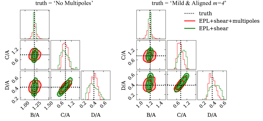
Figure 8: Comparison of model-predicted flux ratios with two different lens models EPL+shear+multipoles (red) and EPL+shear (green), where the true lens has no multipoles (left) and has multipoles of ‘Mild & Aligned $m=4$’ scenario (right). Only image positions are used to constrain the true lens model.

References

- [1] P.A. Ade, N. Aghanim, C. Armitage-Caplan, M. Arnaud, M. Ashdown, F. Atrio-Barandela et al., Planck 2013 results. xvi. cosmological parameters, Astronomy & Astrophysics 571 (2014) A16.
- [2] S. Vegetti, S. Birrer, G. Despali, C. Fassnacht, D. Gilman, Y. Hezaveh et al., Strong gravitational lensing as a probe of dark matter, arXiv preprint arXiv:2306.11781 (2023) .
- [3] S. Mao and P. Schneider, Evidence for substructure in lens galaxies?, Monthly Notices of the Royal Astronomical Society 295 (1998) 587.
- [4] N. Dalal and C.S. Kochanek, Direct detection of cold dark matter substructure, The Astrophysical Journal 572 (2002) 25.
- [5] C.S. Kochanek and N. Dalal, Tests for substructure in gravitational lenses, The Astrophysical Journal 610 (2004) 69.
- [6] J.W. Hsueh, W. Enzi, S. Vegetti, M.W. Auger, C.D. Fassnacht, G. Despali et al., SHARP – VII. New constraints on the dark matter free-streaming properties and substructure abundance from gravitationally lensed quasars, Monthly Notices of the Royal Astronomical Society 492 (2019) 3047.
- [7] D. Gilman, S. Birrer, A. Nierenberg, T. Treu, X. Du and A. Benson, Warm dark matter chills out: constraints on the halo mass function and the free-streaming length of dark matter with eight quadruple-image strong gravitational lenses, MNRAS 491 (2020) 6077.
- [8] D. Gilman, S. Birrer, T. Treu, A. Nierenberg and A. Benson, Probing dark matter structure down to 107 solar masses: flux ratio statistics in gravitational lenses with line-of-sight haloes, Monthly Notices of the Royal Astronomical Society 487 (2019) 5721.
- [9] A.M. Nierenberg, D. Gilman, T. Treu, G. Brammer, S. Birrer, L. Moustakas et al., Double dark matter vision: twice the number of compact-source lenses with narrow-line lensing and the WFC3 grism, Monthly Notices of the Royal Astronomical Society 492 (2019) 5314.
- [10] A. Nierenberg, R. Keeley, D. Sluse, D. Gilman, S. Birrer, T. Treu et al., Jwst lensed quasar dark matter survey i: Description and first results, arXiv preprint arXiv:2309.10101 (2023) .
- [11] J.-W. Hsueh, C.D. Fassnacht, S. Vegetti, J.P. McKean, C. Spingola, M.W. Auger et al., SHARP – II. Mass structure in strong lenses is not necessarily dark matter substructure: a flux ratio anomaly from an edge-on disc in B1555+375, Monthly Notices of the Royal Astronomical Society: Letters 463 (2016) L51.
- [12] C.S. Kochanek, The implications of lenses for galaxy structure, Astrophysical Journal, Part 1 (ISSN 0004-637X), vol. 373, June 1, 1991, p. 354-368. 373 (1991) 354.
- [13] C.S. Trotter, J.N. Winn and J.N. Hewitt, A multipole-taylor expansion for the potential of the gravitational lens mg j0414+ 0534, The Astrophysical Journal 535 (2000) 671.
- [14] O. Möller, P. Hewett and A. Blain, Discs in early-type lensing galaxies: effects on magnification ratios and measurements of h 0, Monthly Notices of the Royal Astronomical Society 345 (2003) 1.
- [15] N.W. Evans and H.J. Witt, Fitting gravitational lenses: truth or delusion, Monthly Notices of the Royal Astronomical Society 345 (2003) 1351.
- [16] A.B. Congdon and C.R. Keeton, Multipole models of four-image gravitational lenses with anomalous flux ratios, Monthly Notices of the Royal Astronomical Society 364 (2005) 1459.
- [17] D. Gilman, A. Agnello, T. Treu, C.R. Keeton and A.M. Nierenberg, Strong lensing signatures of luminous structure and substructure in early-type galaxies, Monthly Notices of the Royal Astronomical Society 467 (2017) 3970.
- [18] L. Van de Vyvere, Gomer, Matthew R., Sluse, Dominique, Xu, Dandan, Birrer, Simon, Galan, Aymeric et al., Tdcosmo - vii. boxyness/discyness in lensing galaxies: Detectability and impact on h0, A&A 659 (2022) A127.
- [19] C. Hao, S. Mao, Z. Deng, X. Xia and H. Wu, Isophotal shapes of elliptical/lenticular galaxies from the sloan digital sky survey, Monthly Notices of the Royal Astronomical Society 370 (2006) 1339.
- [20] D. Gilman, J. Bovy, T. Treu, A. Nierenberg, S. Birrer, A. Benson et al., Strong lensing signatures of self-interacting dark matter in low-mass haloes, MNRAS 507 (2021) 2432.
- [21] A. Laroche, D. Gilman, X. Li, J. Bovy and X. Du, Quantum fluctuations masquerade as haloes: bounds on ultra-light dark matter from quadruply imaged quasars, MNRAS 517 (2022) 1867.
- [22] D. Gilman, A. Benson, J. Bovy, S. Birrer, T. Treu and A. Nierenberg, The primordial matter power spectrum on sub-galactic scales, MNRAS 512 (2022) 3163.
- [23] D. Gilman, Y.-M. Zhong and J. Bovy, Constraining resonant dark matter self-interactions with strong gravitational lenses, Phys. Rev. D. 107 (2023) 103008.
- [24] D. Gilman, S. Birrer, A. Nierenberg and M.S.H. Oh, Turbocharging constraints on dark matter substructure through a synthesis of strong lensing flux ratios and extended lensed arcs, 2024.
- [25] R.E. Keeley, A.M. Nierenberg, D. Gilman, C. Gannon, S. Birrer, T. Treu et al., Jwst lensed quasar dark matter survey ii: Wdm constraints from warm dust flux ratios in 9 systems, in preparation.
- [26] A.J. Shajib, S. Birrer, T. Treu, A. Agnello, E. Buckley-Geer, J. Chan et al., Strides: a 3.9 per cent measurement of the hubble constant from the strong lens system des j0408- 5354, Monthly Notices of the Royal Astronomical Society 494 (2020) 6072.
- [27] T. Schmidt, T. Treu, S. Birrer, A.J. Shajib, C. Lemon, M. Millon et al., Strides: automated uniform models for 30 quadruply imaged quasars, Monthly Notices of the Royal Astronomical Society 518 (2023) 1260.
- [28] S. Birrer and A. Amara, lenstronomy: Multi-purpose gravitational lens modelling software package, Physics of the Dark Universe 22 (2018) 189.
- [29] S. Birrer, A.J. Shajib, D. Gilman, A. Galan, J. Aalbers, M. Millon et al., lenstronomy ii: A gravitational lensing software ecosystem, arXiv preprint arXiv:2106.05976 (2021) .
- [30] J. Sérsic, Influence of the atmospheric and instrumental dispersion on the brightness distribution in a galaxy, Boletin de la Asociacion Argentina de Astronomia La Plata Argentina 6 (1963) 41.
- [31] N. Tessore and R.B. Metcalf, The elliptical power law profile lens, Astronomy & Astrophysics 580 (2015) A79.
- [32] P. Schneider and C. Seitz, Steps towards nonlinear cluster inversion through gravitational distortions. i. basic considerations and circular clusters, arXiv preprint astro-ph/9407032 (1994) .
- [33] P. Schneider, C. Kochanek and J. Wambsganss, Gravitational lensing: strong, weak and micro: Saas-Fee advanced course 33, vol. 33, Springer Science & Business Media (2006).
- [34] M. Meneghetti, Introduction to gravitational lensing: with Python examples, vol. 956, Springer Nature (2021).
- [35] C.R. Keeton, B.S. Gaudi and A.O. Petters, Identifying lenses with small-scale structure. i. cusp lenses, The Astrophysical Journal 598 (2003) 138.
- [36] D. Xu, D. Sluse, L. Gao, J. Wang, C. Frenk, S. Mao et al., How well can cold dark matter substructures account for the observed radio flux-ratio anomalies, Monthly Notices of the Royal Astronomical Society 447 (2015) 3189.
- [37] A. Rest, F.C. van den Bosch, W. Jaffe, H. Tran, Z. Tsvetanov, H.C. Ford et al., Wfpc2 images of the central regions of early-type galaxies. i. the data, The Astronomical Journal 121 (2001) 2431.
- [38] A. Pasquali, I. Ferreras, N. Panagia, E. Daddi, S. Malhotra, J.E. Rhoads et al., The structure and star formation history of early-type galaxies in the ultra deep field/grapes survey, The Astrophysical Journal 636 (2006) 115.
- [39] K. Mitsuda, M. Doi, T. Morokuma, N. Suzuki, N. Yasuda, S. Perlmutter et al., Isophote shapes of early-type galaxies in massive clusters at z 1 and 0, The Astrophysical Journal 834 (2017) 109.
- [40] R. Narayan and M. Bartelmann, Lectures on gravitational lensing, arXiv preprint astro-ph/9606001 (1996) .
- [41] A.J. Shajib, S. Birrer, T. Treu, M. Auger, A. Agnello, T. Anguita et al., Is every strong lens model unhappy in its own way? uniform modelling of a sample of 13 quadruply+ imaged quasars, Monthly Notices of the Royal Astronomical Society 483 (2019) 5649.
- [42] A. Agnello, H. Lin, N. Kuropatkin, E. Buckley-Geer, T. Anguita, P.L. Schechter et al., DES meets Gaia: discovery of strongly lensed quasars from a multiplet search, Monthly Notices of the Royal Astronomical Society 479 (2018) 4345.
- [43] A. Krone-Martins, L. Delchambre, O. Wertz, C. Ducourant, F. Mignard, R.T.J. Klüter et al., Gaia gral: Gaia dr2 gravitational lens systems. i. new quadruply imaged quasar candidates around known quasars, Astronomy and Astrophysics-A&A 616 (2018) id.
- [44] D. Gilman, S. Birrer, T. Treu, C.R. Keeton and A. Nierenberg, Probing the nature of dark matter by forward modelling flux ratios in strong gravitational lenses, Monthly Notices of the Royal Astronomical Society 481 (2018) 819.
- [45] A. Etherington, J.W. Nightingale, R. Massey, S.-I. Tam, X. Cao, A. Niemiec et al., Strong gravitational lensing’s ‘external shear’ is not shear, 2023.
- [46] L. Van de Vyvere, D. Sluse, S. Mukherjee, D. Xu and S. Birrer, The impact of mass map truncation on strong lensing simulations, Astronomy & Astrophysics 644 (2020) A108.
- [47] R. Bender, S. Doebereiner and C. Moellenhoff, Isophote shapes of elliptical galaxies. i-the data, Astronomy and Astrophysics Supplement Series (ISSN 0365-0138), vol. 74, no. 3, Sept. 1988, p. 385-426. 74 (1988) 385.