Level attraction from interference in two-tone driving
Abstract
Coherent and dissipative couplings, respectively characterised by energy level repulsion and attraction, each have different applications for quantum information processing. Thus, a system in which both coherent and dissipative couplings are tunable on-demand and in-situ is tantalising. A first step towards this goal is the two-tone driving of two bosonic modes, whose experimental signature was shown to exhibit controllable level repulsion and attraction by changing the phase and amplitude of one drive. However, whether the underlying physics is that of coherent and dissipative couplings has not been clarified, and cannot be concluded solely from the measured resonances (or anti-resonances) of the system. Here, we show how the physics at play can be analysed theoretically. Combining this theory with realistic finite-element simulations, we deduce that the observation of level attraction originates from interferences due to the measurement setup, and not dissipative coupling. Beyond the clarification of a novel origin for level attraction attributed to interference, our work demonstrate how effective Hamiltonians can be derived to appropriately describe the physics.
Introduction.
The coherent coupling between two systems corresponds to the coherent exchange of energy between them, and is characterised by energy level repulsion (also known as normal-mode splitting or an anti-crossing). This phenomenon is ubiquitous in physics, spanning the classical coupling of two harmonic oscillators [1] to the coupling of bosonic quasi-particles with two-level systems [2] or other bosonic excitations [3]. With respect to quantum information processing, coherent coupling allows to convert quantum information between light and solid state degrees of freedom, and is therefore an elementary building-block of quantum communication [4, 5, 6]. On the other hand, dissipative coupling [7, 8, 9], characterised by energy level attraction instead, arises due to the indirect coupling of two modes mediated by a common reservoir [10, 11, 12] (e.g. a strongly dissipative auxiliary mode [13], a photonic environment [14, 15, 16], metallic leads [17]). The merging of energy levels characterising dissipative couplings leads to exceptional points [18, 19, 20, 21], which can be useful for topological energy transfer [22], and improved sensitivity for quantum metrology and quantum sensing applications [23, 24]. Furthermore, balancing coherent and dissipative couplings, using dissipation engineering and synthetic gauge fields, allows to break time-reversal symmetry and thus create non-reciprocal devices [10, 11, 12, 25, 26, 27, 28]. Therefore, building a system in which both coherent and dissipative couplings co-exist and are tunable would be useful to access all the aforementioned applications in a unique versatile platform.
Such a system, due to the presence of both coherent and dissipative couplings, should have an energy spectrum exhibiting both level repulsion and level attraction. Two reflection experiments [29, 30], in which two coherently-coupled bosonic modes were simultaneously driven, suggested such an energy level structure (and hence the presence of coherent and dissipative couplings). Indeed, it is usually expected that the response of a system to excitations at frequencies close to their normal modes leads to resonances (or anti-resonances), with various possible line shapes informing on the underlying physics [31, 32]. However, inspection of the experimental signature alone is not sufficient because it may not be related to the energy levels. Additionally, while dissipative coupling implies level attraction in a variety of platforms such as optomechanics [33], Aharonov-Bohm interferometers [17] or semiconductor microcavities [16] and micropillar lasers [34], alternative physics can also lead to level attraction, as exemplified in optomechanics [35] or spinor condensates [36]. For all these reasons, the physics at play in two-tone driving remains unclear.
In this letter, we model a two-tone driving experiment, similar to those of [29, 30]. Our starting point is the Hamiltonian of two coherently coupled bosonic modes, whose spectrum is that of level repulsion. To model the two-tone driving and the experimentally accessible quantities, we use quantum Langevin equations (QLEs) and the input-output formalism [37]. This theoretical treatment allows to find an analytical expression for the experimental signature, where both level repulsion and attraction can occur. Importantly, we show analytically and using finite element simulations, that level attraction can be attributed to an anti-resonance due to the destructive interference between the reflection and transmission coefficients. To clarify the physics, we derive the open-system effective Hamiltonian of the two-tone driven system, and show that the physics remains exclusively that of coherent coupling, despite the observation of level attraction.
Quantum Langevin equations.
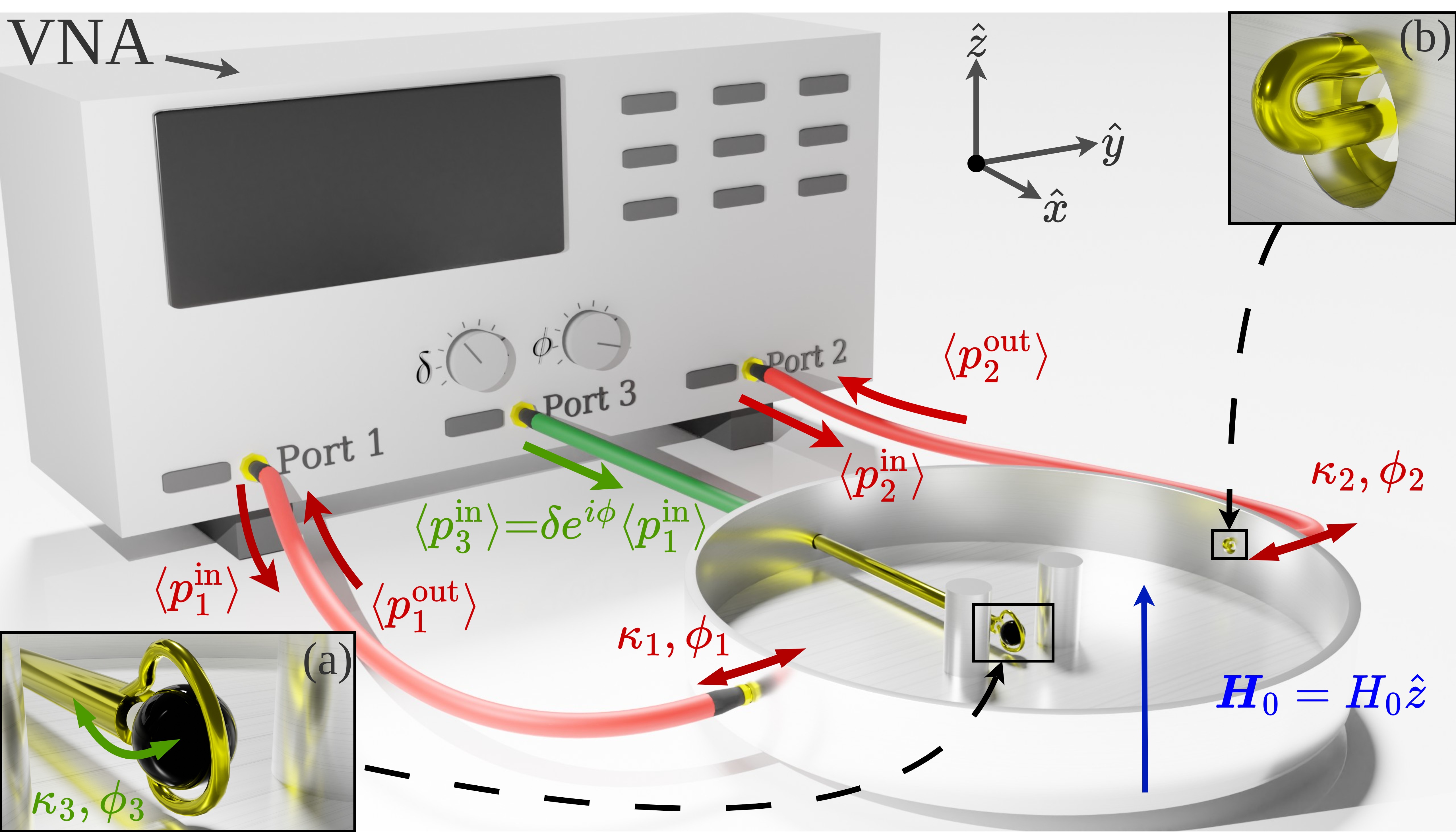
We consider the experimental setup of fig. 1, where a ferromagnetic sphere made of Yttrium-Iron-Garnet (YIG) is placed inside a microwave cavity. The second-quantised Hamiltonian of the system enclosed inside the cavity is that of the lowest-order magnon mode (quantised spin wave) coupled to a single cavity mode, described by [9]
| (1) |
where is the (complex) coherent coupling strength [39, 40] between the cavity mode (operators ) and the magnon mode (operators ). The frequency of the cavity mode is fixed by the cavity’s geometry, while the ferromagnetic resonance of the magnon is tuned by a static magnetic field as where GHz/T is the gyromagnetic ratio.
The quantum Langevin equations (QLEs) allow to model the coupling of the cavity system described by eq. 1 to the environment, to model intrinsic dissipation or external drives. To model the intrinsic damping of the cavity mode and the magnon mode , we assume that they each couple to their own bosonic bath with coupling constants and . As per fig. 1, the cavity system described by eq. 1 is coupled to three ports , labelled from 1 to 3, where the first two ports couple only to the cavity mode (with real-valued coupling constants and and phases [41]) and the third couples only to the magnon mode (real-valued coupling constant with phase ). Physically, the coupling of the magnon to port 3 is due to the Zeeman interaction with the magnetic field created by the loop of port 3. The QLE for the cavity and magnon modes then read [42]
| (2) | ||||
| (3) |
where and . In the QLEs, and account for intrinsic damping and have zero mean , while represent the coupling to the ports.
Two-tone reflection and transmission.
We now assume that and correspond to coherent drives at the same frequency, albeit with a phase and amplitude difference written . We also perform a semi-classical approximation and neglect quantum fluctuations, which amounts to only considering expectation values. Using the input-output formalism [42], the reflection at Port 1 when Port 3 is active is found to be
| (4) | ||||
| (5) |
where and . By comparing with the expressions of the standard S-parameters [42], we note that the reflection can also be written which is expected given the linearity of the problem.
For , the reflection coefficient can be greater than one, because it is only normalised to the input power from Port 1, thus neglecting that of Port 3. Following the setup of fig. 1, and taking the power out of Port 1 as a reference, the VNA outputs a power , so we can renormalise the reflection to . Similarly, we can calculate the normalised transmission coefficient through Port 2 when both Port 1 and Port 3 are active, and we find [43]
| (6) |
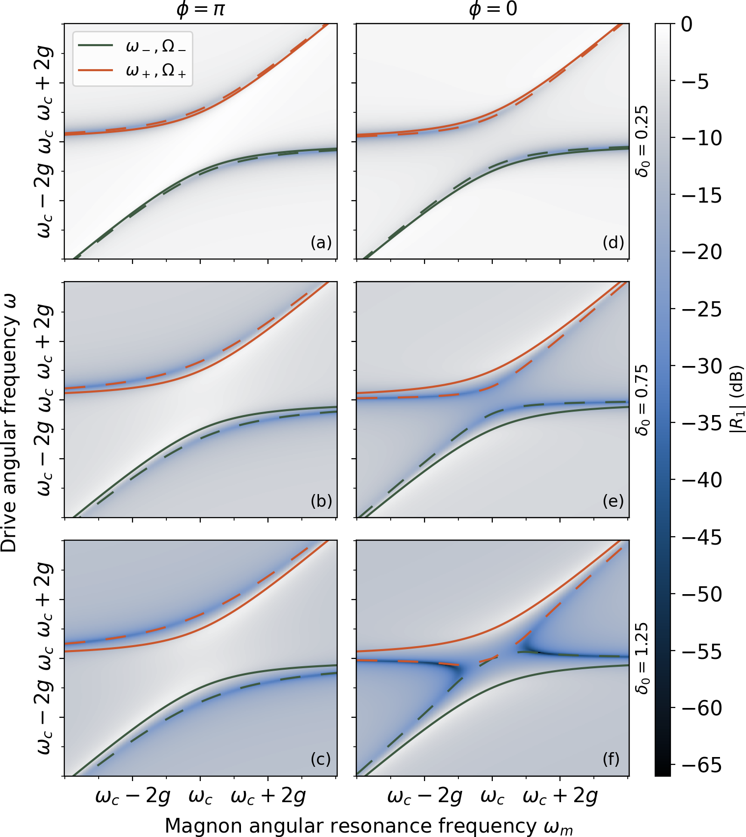
We plot in fig. 2 and in fig. 3 with the parameters GHz, MHz, MHz, MHz, MHz, and . The reflection exhibits controllable level repulsion and attraction depending on the amplitude of the drives and the dephasing , mirroring the experimental results of [29, 30]. On the other hand, we notice that the transmission only shows level repulsion, despite the system being driven in exactly the same way: between and , only the measurement location changes, and thus the physics should be the same.
Analysis of the two-tone reflection coefficient.
An advantage of the input-output formalism is that it allows us to understand analytically the spectral features of fig. 2. Indeed, by writing in terms of a nominator and a denominator , the denominator can be factorised as
| (7) | ||||
| (8) |
where
| (9) |
are the complex-valued solutions of the quadratic eq. 7.
On the other hand, the nominator can be written as
| (10) |
where we defined and
| (11) |
with is the phase of the complex number . Comparing eqs. 7 and 10, we see that the nominator can be factored similarly to the denominator as , where the complex frequencies are formally identical to eq. 9, after replacing and . Finally, we obtain
| (12) |
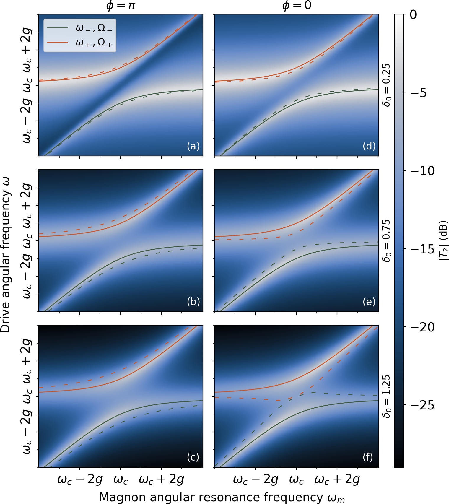
For small dissipation rates , the imaginary part of is small compared to its real part. Therefore, in eq. 12, when is close to , the denominator of almost vanishes, leading to a resonance behaviour (maxima) of . Furthermore, correspond to the spectrum of the Hamiltonian of eq. 1, and hence this resonance behaviour is expected to give information about the spectrum of the closed-system. As shown by the solid lines in figs. 2 and 3, the spectrum is that of coherent coupling, characterised by energy level repulsion with an angular frequency gap . Hence, the denominator of , or equivalently its resonances, does inform on the underlying physics.
The situation is different for the nominator of . Indeed, while the expressions of and are formally identical, the effective coupling strength for is complex-valued (while it is real-valued, , for ) which can lead to level attraction. To see this more clearly, it is convenient to introduce the effective amplitude and the effective phase of Port 3. We can then rewrite eq. 11 as
| (13) |
Therefore, when the effective coupling strength is real-valued and increases as increases, leading to an increase of level repulsion (see the dashed lines in the first column of fig. 2). On the other hand, when , the effective coupling strength is real-valued when and diminishes when increases. Eventually, when , the coupling strength becomes purely imaginary due to taking the square root of a negative number, leading to level attraction. In the limiting case where , we have and we obtain two uncoupled anti-resonances (an horizontal one at the cavity mode frequency and a diagonal one at the magnon’s frequency ). As can be seen from the dashed lines in fig. 2, these spectral features indeed correspond to anti-resonances (zeros of the nominator corresponding to minima of ) at the frequencies . Physically, these frequencies are determined by the interference between the nominators of and since . Hence, the input-output formalism shows that while the denominator of informs on the physics, the nominator is interference-based. Indeed, the denominator of both and are identical, leading to similar resonant behaviour following the coherent coupling spectrum. However, their anti-resonance behaviours differ because their nominators differ [43].
Numerical finite element results.
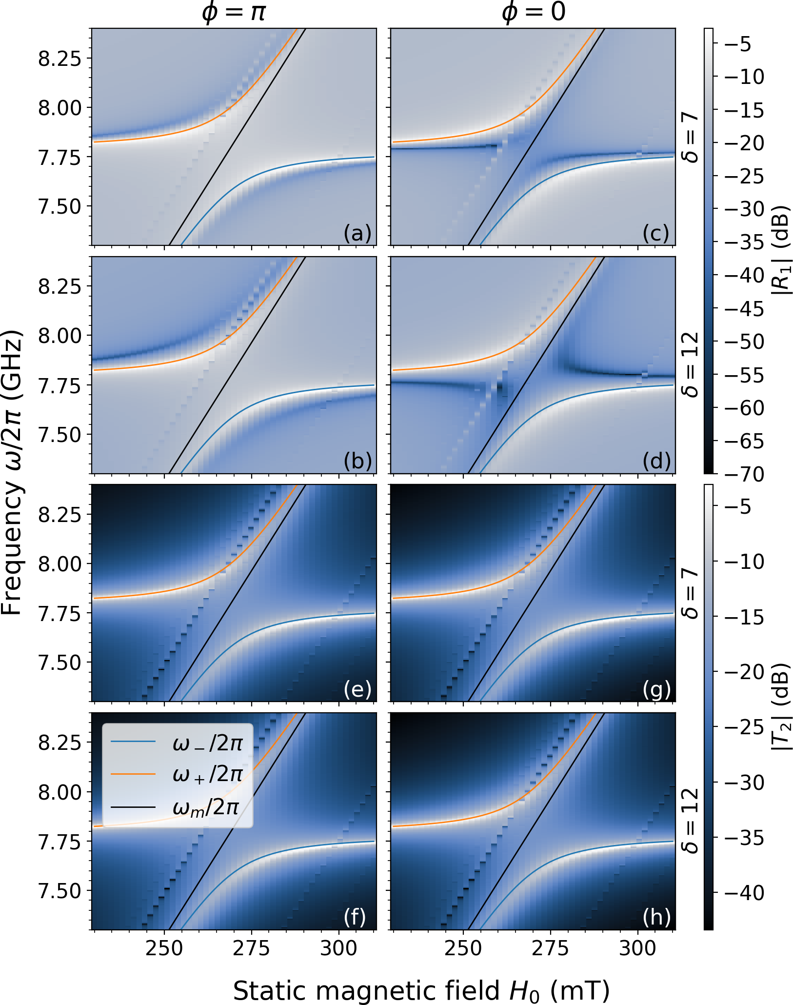
The input-output formalism provides interesting insights thanks to the resulting analytical expressions. However, it remains a toy-model of a two-tone driving experiment. Instead, a realistic modelling, taking into account the geometry of the cavity and of the ports, can be perfomed using COMSOL Multiphysics®, a finite element modelling software. We use a two-post re-entrant cavity [44, 45], similar to that sketched in fig. 1, in which the loop antenna of Port 3 is inserted from the bottom of the cavity [46]. At the location of the YIG sphere, the cavity mode’s magnetic field is purely along the axis [38]. In our analysis, we assumed that Port 3 does not couple to the cavity mode, which requires us to orient the loop antenna so that it generates a magnetic field orthogonal to the cavity mode. Thus, noting the normal to the plane of the loop, we need to be in the plane. Furthermore, since only the components orthogonal to the static magnetic field contribute to the coupling between Port 3 and the magnon, is maximum when .
We first numerically calculated the S parameters for different values of using COMSOL [46]. From these two parameters, we can plot and after normalising and , and we obtain the results of fig. 4, which successfully reproduce the input-output theory results of figs. 2 and 3. As a further verification, we also performed a fully two-tone experiment in COMSOL for , and the results were identical to those of the second and fourth rows of fig. 4.
Effective Hamiltonian for the open system.
We have now confirmed that the resonances of and follow energy level repulsion, suggesting coherent coupling physics. However, one may worry that the physics of the two-tone driven system is different from the physics of the closed-system Hamiltonian of eq. 1, which not include the coherent drives. To derive the effective Hamiltonian, we write the QLEs eqs. 2 and 3 in the semi-classical approximation where operators are replaced by their expectation values. Recalling that , the QLEs read
| (14) | ||||
| (15) |
In both a reflection and transmission measurement, port 2 is not driven, so we set . On the other hand, and correspond to a coherent drive at frequency , with amplitude and . Thus, further defining and , the QLEs become [42]
| (16) | ||||
| (17) |
From these equations, we find that the effective non-hermitian Hamiltonian (recall that )
| (18) | ||||
where stands for the hermitian conjugate terms, gives Heisenberg equations of motion identical to eqs. 16 and 17. Thus, the physics described by eq. 18 is identical to that given by the QLEs. After a rotating frame transformation to remove the time-dependence and displacement operations [47], this Hamiltonian is unitarily equivalent to
| (19) |
Physical interpretation and conclusion.
Formally similar to the closed-system Hamiltonian of eq. 1, this effective Hamiltonian describes the coherent coupling physics between photons and magnon, and thus its spectrum corresponds to level repulsion. Since describes the physics of the cavity system in the presence of coherent drives, we conclude that the physics of two-tone driving indeed corresponds to coherent coupling, even though the reflection coefficient can show level attraction due to interference-based anti-resonances. Therefore, the anti-resonance frequencies (dashed lines in fig. 2) do not correspond to the spectrum of the system, which are instead given by (solid lines in fig. 2).
It is worth noting that here, the anti-resonances leading to level attraction come from interferences between and . However, anti-resonances can also appear in a one-tone driven system as experimentally demonstrated by Rao et al. [48]. Notably, these anti-resonances can exhibit different coupling behaviour recently analysed by [41], and suggest energy level repulsion and attraction with a magnon mode. These behaviours are associated with the numerators of the transmission coefficient, and therefore they are not associated to a physical coherent and dissipative coupling. Importantly, it is incorrect to derive an effective Hamiltonian from this numerator alone, as it is not associated with a physical dynamics.
To conclude, we have showed that when two bosonic modes are simultaneously driven, the resonances in reflection and transmission indeed inform on the normal modes of the system, while the observed anti-resonances are due to interference physics, and are unrelated to the coupled system. We note that while two-tone driving do not correspond to the in-situ control of coherent and dissipative couplings, achieving it is still a relevant research direction. Finally, we note that while we considered a cavity magnonics system as a physical realisation of two coupled bosonic modes, many other systems, such as intersubband polaritons [49] or cavity optomechanics in the red-detuned regime [50], reduce to a similar Hamiltonian. Indeed, the model Hamiltonian of eq. 1 is essentially the Dicke model [51] after employing the Holstein-Primakoff transformation [52] and then the rotating wave approximation [53]. Hence, the derivations employed here are very general and may prove useful to analyse the physics in other systems.
Acknowledgements.
We acknowledge financial support from Thales Australia and Thales Research and Technology. The scientific colour map oslo [54] is used in this study to prevent visual distortion of the data and exclusion of readers with colourvision deficiencies [55]. This work is part of the research program supported by the European Union through the European Regional Development Fund (ERDF), by the Ministry of Higher Education and Research, Brittany and Rennes Métropole, through the CPER SpaceTech DroneTech, by Brest Métropole, and the ANR projects ICARUS (ANR-22-CE24-0008) and MagFunc (ANR-20-CE91-0005).References
- Novotny [2010] L. Novotny, Strong coupling, energy splitting, and level crossings: A classical perspective, American Journal of Physics 78, 1199 (2010).
- Weisbuch et al. [1992] C. Weisbuch, M. Nishioka, A. Ishikawa, and Y. Arakawa, Observation of the coupled exciton-photon mode splitting in a semiconductor quantum microcavity, Physical Review Letters 69, 3314 (1992).
- Dobrindt et al. [2008] J. M. Dobrindt, I. Wilson-Rae, and T. J. Kippenberg, Parametric normal-mode splitting in cavity optomechanics, Physical Review Letters 101, 263602 (2008).
- Gisin and Thew [2007] N. Gisin and R. Thew, Quantum communication, Nature Photonics 1, 165 (2007).
- Kimble [2008] H. J. Kimble, The quantum internet, Nature 453, 1023 (2008).
- Lachance-Quirion et al. [2019] D. Lachance-Quirion, Y. Tabuchi, A. Gloppe, K. Usami, and Y. Nakamura, Hybrid quantum systems based on magnonics, Applied Physics Express 12, 070101 (2019).
- Lu et al. [2023a] C. Lu, B. Turner, Y. Gui, J. Burgess, J. Xiao, and C.-M. Hu, An experimental demonstration of level attraction with coupled pendulums, American Journal of Physics 91, 585 (2023a).
- Wang and Hu [2020] Y.-P. Wang and C.-M. Hu, Dissipative couplings in cavity magnonics, Journal of Applied Physics 127, 130901 (2020).
- Harder et al. [2021] M. Harder, B. M. Yao, Y. S. Gui, and C.-M. Hu, Coherent and dissipative cavity magnonics, Journal of Applied Physics 129, 201101 (2021).
- Wang et al. [2019] Y.-P. Wang, J. Rao, Y. Yang, P.-C. Xu, Y. Gui, B. Yao, J. You, and C.-M. Hu, Nonreciprocity and unidirectional invisibility in cavity magnonics, Physical Review Letters 123, 127202 (2019).
- Metelmann and Clerk [2015] A. Metelmann and A. A. Clerk, Nonreciprocal photon transmission and amplification via reservoir engineering, Physical Review X 5, 021025 (2015).
- Clerk [2022] A. Clerk, Introduction to quantum non-reciprocal interactions: from non-hermitian hamiltonians to quantum master equations and quantum feedforward schemes, SciPost Physics Lecture Notes 10.21468/scipostphyslectnotes.44 (2022).
- Yu et al. [2019] W. Yu, J. Wang, H. Yuan, and J. Xiao, Prediction of attractive level crossing via a dissipative mode, Physical Review Letters 123, 227201 (2019).
- Yao et al. [2019a] B. Yao, T. Yu, Y. S. Gui, J. W. Rao, Y. T. Zhao, W. Lu, and C.-M. Hu, Coherent control of magnon radiative damping with local photon states, Communications Physics 2, 10.1038/s42005-019-0264-z (2019a).
- Yao et al. [2019b] B. Yao, T. Yu, X. Zhang, W. Lu, Y. Gui, C.-M. Hu, and Y. M. Blanter, The microscopic origin of magnon-photon level attraction by traveling waves: Theory and experiment, Physical Review B 100, 214426 (2019b).
- Bleu et al. [2024] O. Bleu, K. Choo, J. Levinsen, and M. M. Parish, Dissipative light-matter coupling and anomalous dispersion in nonideal cavities, Physical Review A 109, 023707 (2024).
- Kubala and König [2002] B. Kubala and J. König, Flux-dependent level attraction in double-dot aharonov-bohm interferometers, Physical Review B 65, 245301 (2002).
- Heiss [2012] W. D. Heiss, The physics of exceptional points, Journal of Physics A: Mathematical and Theoretical 45, 444016 (2012).
- Zhang et al. [2017] D. Zhang, X.-Q. Luo, Y.-P. Wang, T.-F. Li, and J. Q. You, Observation of the exceptional point in cavity magnon-polaritons, Nature Communications 8, 10.1038/s41467-017-01634-w (2017).
- Zhang and You [2019] G.-Q. Zhang and J. Q. You, Higher-order exceptional point in a cavity magnonics system, Physical Review B 99, 054404 (2019).
- Hurst and Flebus [2022] H. M. Hurst and B. Flebus, Non-hermitian physics in magnetic systems, Journal of Applied Physics 132, 10.1063/5.0124841 (2022), arXiv:2209.03946 [cond-mat.mes-hall] .
- Xu et al. [2016] H. Xu, D. Mason, L. Jiang, and J. G. E. Harris, Topological energy transfer in an optomechanical system with exceptional points, Nature 537, 80 (2016).
- Cao and Yan [2019] Y. Cao and P. Yan, Exceptional magnetic sensitivity of pt-symmetric cavity magnon polaritons, Physical Review B 99, 214415 (2019).
- Yu et al. [2020] T. Yu, H. Yang, L. Song, P. Yan, and Y. Cao, Higher-order exceptional points in ferromagnetic trilayers, Physical Review B 101, 144414 (2020).
- Koch et al. [2010] J. Koch, A. A. Houck, K. L. Hur, and S. M. Girvin, Time-reversal-symmetry breaking in circuit-QED-based photon lattices, Physical Review A 82, 043811 (2010).
- Sliwa et al. [2015] K. Sliwa, M. Hatridge, A. Narla, S. Shankar, L. Frunzio, R. Schoelkopf, and M. Devoret, Reconfigurable josephson circulator/directional amplifier, Physical Review X 5, 041020 (2015).
- Fang et al. [2017] K. Fang, J. Luo, A. Metelmann, M. H. Matheny, F. Marquardt, A. A. Clerk, and O. Painter, Generalized non-reciprocity in an optomechanical circuit via synthetic magnetism and reservoir engineering, Nature Physics 13, 465 (2017).
- Huang et al. [2021] X. Huang, C. Lu, C. Liang, H. Tao, and Y.-C. Liu, Loss-induced nonreciprocity, Light: Science & Applications 10, 30 (2021).
- Boventer et al. [2019] I. Boventer, M. Kläui, R. Macêdo, and M. Weides, Steering between level repulsion and attraction: broad tunability of two-port driven cavity magnon-polaritons, New Journal of Physics 21, 125001 (2019).
- Boventer et al. [2020] I. Boventer, C. Dörflinger, T. Wolz, R. Macêdo, R. Lebrun, M. Kläui, and M. Weides, Control of the coupling strength and linewidth of a cavity magnon-polariton, Physical Review Research 2, 013154 (2020).
- Bärnthaler et al. [2010] A. Bärnthaler, S. Rotter, F. Libisch, J. Burgdörfer, S. Gehler, U. Kuhl, and H.-J. Stöckmann, Probing decoherence through fano resonances, Physical Review Letters 105, 056801 (2010).
- Limonov et al. [2017] M. F. Limonov, M. V. Rybin, A. N. Poddubny, and Y. S. Kivshar, Fano resonances in photonics, Nature Photonics 11, 543 (2017).
- Lu et al. [2023b] Q. Lu, J. Guo, Y.-L. Zhang, Z. Fu, L. Chen, Y. Xiang, and S. Xie, Level attraction due to dissipative phonon–phonon coupling in an opto-mechano-fluidic resonator, ACS Photonics 10, 699 (2023b).
- Khanbekyan et al. [2015] M. Khanbekyan, H. A. M. Leymann, C. Hopfmann, A. Foerster, C. Schneider, S. Höfling, M. Kamp, J. Wiersig, and S. Reitzenstein, Unconventional collective normal-mode coupling in quantum-dot-based bimodal microlasers, Physical Review A 91, 043840 (2015).
- Bernier et al. [2018] N. R. Bernier, L. D. Tóth, A. K. Feofanov, and T. J. Kippenberg, Level attraction in a microwave optomechanical circuit, Physical Review A 98, 023841 (2018).
- Bernier et al. [2014] N. R. Bernier, E. G. Dalla Torre, and E. Demler, Unstable avoided crossing in coupled spinor condensates, Physical Review Letters 113, 065303 (2014).
- Gardiner and Collett [1985] C. W. Gardiner and M. J. Collett, Input and output in damped quantum systems: Quantum stochastic differential equations and the master equation, Physical Review A 31, 3761 (1985).
- Bourhill et al. [2020] J. Bourhill, V. Castel, A. Manchec, and G. Cochet, Universal characterization of cavity–magnon polariton coupling strength verified in modifiable microwave cavity, Journal of Applied Physics 128, 073904 (2020).
- Flower et al. [2019] G. Flower, M. Goryachev, J. Bourhill, and M. E. Tobar, Experimental implementations of cavity-magnon systems: from ultra strong coupling to applications in precision measurement, New Journal of Physics 21, 095004 (2019).
- Gardin et al. [2023] A. Gardin, J. Bourhill, V. Vlaminck, C. Person, C. Fumeaux, V. Castel, and G. C. Tettamanzi, Manifestation of the coupling phase in microwave cavity magnonics, Physical Review Applied 19, 054069 (2023), arXiv:2212.05389 [quant-ph] .
- Bourcin et al. [2024] G. Bourcin, A. Gardin, J. Bourhill, V. Vlaminck, and V. Castel, Level attraction in a quasi-closed cavity, (2024), type: article, arxiv:2402.06258 [quant-ph] .
- [42] See supplemental material at [url] for the derivation of the quantum langevin equation and the input-output theory.
- [43] See supplemental material at [url] for the expression of the transmission and its plot.
- Goryachev et al. [2014] M. Goryachev, W. G. Farr, D. L. Creedon, Y. Fan, M. Kostylev, and M. E. Tobar, High-cooperativity cavity qed with magnons at microwave frequencies, Phys. Rev. Applied 2, 054002 (2014).
- Kostylev et al. [2016] N. Kostylev, M. Goryachev, and M. E. Tobar, Superstrong coupling of a microwave cavity to yttrium iron garnet magnons, Applied Physics Letters 108, 062402 (2016).
- [46] See supplemental material at [url] for more details on the cavity used in the simulations and its characterisation.
- [47] See supplemental material at [url] for the details of the transformations.
- Rao et al. [2019] J. W. Rao, C. H. Yu, Y. T. Zhao, Y. S. Gui, X. L. Fan, D. S. Xue, and C.-M. Hu, Level attraction and level repulsion of magnon coupled with a cavity anti-resonance, New Journal of Physics 21, 065001 (2019).
- Ciuti et al. [2005] C. Ciuti, G. Bastard, and I. Carusotto, Quantum vacuum properties of the intersubband cavity polariton field, Physical Review B 72, 115303 (2005).
- Aspelmeyer et al. [2014] M. Aspelmeyer, T. J. Kippenberg, and F. Marquardt, Cavity optomechanics, Reviews of Modern Physics 86, 1391 (2014).
- Hepp and Lieb [1973] K. Hepp and E. H. Lieb, On the superradiant phase transition for molecules in a quantized radiation field: the dicke maser model, Annals of Physics 76, 360 (1973).
- Holstein and Primakoff [1940] T. Holstein and H. Primakoff, Field dependence of the intrinsic domain magnetization of a ferromagnet, Phys. Rev. 58, 1098 (1940).
- Le Boité [2020] A. Le Boité, Theoretical methods for ultrastrong light–matter interactions, Advanced Quantum Technologies 3, 1900140 (2020), https://onlinelibrary.wiley.com/doi/pdf/10.1002/qute.201900140 .
- Crameri [2021] F. Crameri, Scientific colour maps (2021).
- Crameri et al. [2020] F. Crameri, G. E. Shephard, and P. J. Heron, The misuse of colour in science communication, Nature Communications 11, 10.1038/s41467-020-19160-7 (2020).