Defending Spiking Neural Networks against Adversarial Attacks through Image Purification

Abstract

Spiking Neural Networks (SNNs) aim to bridge the gap between neuroscience and machine learning by emulating the structure of the human nervous system. However, like convolutional neural networks, SNNs are vulnerable to adversarial attacks. To tackle the challenge, we propose a biologically inspired methodology to enhance the robustness of SNNs, drawing insights from the visual masking effect and filtering theory. First, an end-to-end SNN-based image purification model is proposed to defend against adversarial attacks, including a noise extraction network and a non-blind denoising network. The former network extracts noise features from noisy images, while the latter component employs a residual U-Net structure to reconstruct high-quality noisy images and generate clean images. Simultaneously, a multi-level firing SNN based on Squeeze-and-Excitation Network is introduced to improve the robustness of the classifier. Crucially, the proposed image purification network serves as a pre-processing module, avoiding modifications to classifiers. Unlike adversarial training, our method is highly flexible and can be seamlessly integrated with other defense strategies. Experimental results on various datasets demonstrate that the proposed methodology outperforms state-of-the-art baselines in terms of defense effectiveness, training time, and resource consumption.

123

1 Introduction

Over the past decade, Artificial Neural Networks (ANNs) have demonstrated remarkable performance in computer vision [15], speech recognition [4], and natural language processing [33]. However, the static activation values of ANNs neurons deviate from the dynamic characteristics of biological neurons. In contrast, Spiking Neural Networks (SNNs) offer a more biologically realistic approach, where neurons communicate through discrete events or spikes. This event-driven mechanism facilitates asynchronous operation, enabling low power consumption [6]. Especially in power-constrained scenarios, such as edge computing or mobile applications, the benefits of SNNs can be substantial.

Recent advancements in training algorithms for SNNs [34, 30, 17] have narrowed the gap between SNNs and ANNs in real applications. Besides, the emergence of neuromorphic computing system further enhances the performance advantages of SNNs, making them a viable option for deployment in resource-constrained environments. Nonetheless, the deployment of SNNs on terminals raises concerns about their reliability, particularly in the face of adversarial attacks.

Adversarial attacks, where imperceptible perturbations are added to clean images, pose a significant threat to the security of SNN models. But in the real world, biological neural systems that SNNs aim to emulate demonstrate resilience in the face of various perturbations and noise, and rarely exhibit the susceptibilities observed in ANNs. This discrepancy motivates us to explore novel structures to enhance the robustness of SNNs and further diminish the gap between artificial and real neural systems.

Many defense techniques, such as adversarial training [12], defensive distillation [25], and gradient regularization [28], have been proposed for ANNs. These approaches apply either additional training or modifications of input data and gradients to conquer specific attacks. Drawing inspiration from defense methods used in ANNs, researchers have recently developed defense schemes specifically for SNNs to adapt them to SNN-compatible, including adversarial training [7] and encoding input information [1]. Although these works have improved the robustness of SNNs, challenges like resource-intensive processes and prolonged computational times still exist.

Moreover, most SNN researches focus on specific functions of the nervous system, neglecting that the nervous system is a complex entity consisting of multiple interconnected and interacting neural networks. Therefore, in this work, we attempt to build a computationally efficient framework for SNN adversarial defense.

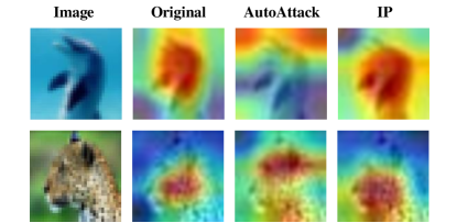
Figure 1: Neuron activation of SENet18-SNN under different cases. IP denotes the proposed image purification network, and input images are selected from CIFAR-100.

To achieve robustness, it is crucial to investigate how the adversarial attack impacts SNNs. We employ the visualization tool [29] to analyze the potential effects. In Figure 1, we observe the activation shifts of a model when presented with clean and adversarial images, respectively. It is evident that adversarial attacks mislead the model’s output by obfuscating the neuron activation. We believe that the essence of adversarial attacks lie in introducing adversarial noise, which finally induces changes in neuron activation. Therefore, the objective of the work is to eliminate the effects of the incurred noise, minimize the occurrence of neuron errors, and ultimately enhance the robustness of the SNN network.

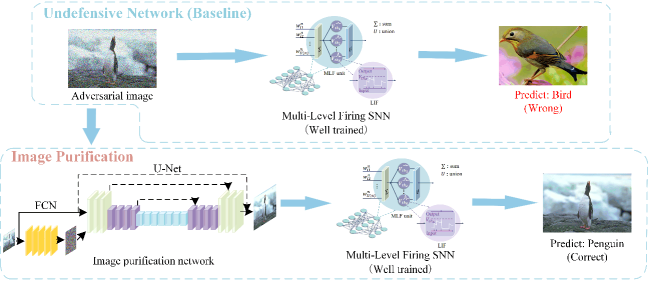
Figure 2: The main idea of our end-to-end image purification network to defend adversarial examples.

SNNs possess inherent robustness compared to CNNs and exhibit robust resistance to slight disturbances [31]. Consequently, alterations in certain original features caused by image reconstruction have a minimal impact on the target network. To this end, we propose an SNN-based image purification network serving as a pre-processing module to eliminate imperceptible noise without compromising classifier accuracy. At the same time, we use Multi-Level Firing to reduce the number of error pulses and enhance the inherent robustness of the network. The basic idea of our methodology is depicted in Figure 2. Key technical contributions of this work are listed as follows.

• An SNN-based image purification model is proposed to defend adversarial examples, where the Fully Convolutional Network (FCN) extracts the noise information from adversarial images. Meanwhile, the U-Net reconstructs the noise image to get the original one. To the best of our knowledge, this is the first SNN-based image purification model to defend against adversarial attacks.

• The proposed image purification model is an end-to-end pre-processing module, which is highly flexible and can be integrated in series with the classifier to form the entire defense network. Once the image purification network is well trained with an arbitrary classifier, it can be seamlessly transferred to other similar classifiers.

• Multi-level firing SNNs based on Squeeze-and-Excitation Networks (SENets) are developed to enhance the robustness of the network structure. Moreover, a unified learning algorithm with a loss function is devised to fit the characteristics of SNNs.

• The image purification model is fully validated on various datasets. Experimental results demonstrate that, compared with state-of-the-art works, the proposed end-to-end methodology provides superior defense effectiveness and significantly reduces training time and resource consumption.

The rest of the paper is organized as follows. Section 2 presents an overview of related works. Section 3 gives the preliminaries. Section 4 describes the proposed methodology in detail. Section 5 lists the experimental results, followed by the conclusions in Section 6.

2 Related Works

We investigate related works in three domains: attack methods for generating adversarial examples, defense approaches against adversarial examples, and the robustness of SNNs.

2.1 Adversarial Attack

Fast Gradient Sign Method (FGSM) [12] is an efficient one-step method for rapidly generating adversarial examples, which maximizes the loss function $\mathcal{L}$ by introducing perturbations along the gradient’s ascending direction. The FGSM perturbed input $\boldsymbol{x}_{adv}$ is updated as:

$$\boldsymbol{x}_{adv}=\boldsymbol{x}+\epsilon\cdot sign(\nabla_{\boldsymbol{x}}\mathcal{L}(\boldsymbol{x},\boldsymbol{y};\boldsymbol{w})),$$ (1)

where $\boldsymbol{x}$ is the clean image, $\boldsymbol{y}$ refers to the true label, and $\epsilon$ denotes the size of the allowed adversarial perturbation. Meanwhile, $\boldsymbol{w}$ represents the network weights.

Iterative FGSM (I-FGSM) [32] is an iterative variant of FGSM, enhancing attack performance through multiple iterations. The adversarial example $\boldsymbol{x}_{adv}$ is generated as:

$$\boldsymbol{x}_{t+1}=clip_{\epsilon}\{\boldsymbol{x}_{t}+\frac{\epsilon}{step}\cdot sign(\nabla_{\boldsymbol{x}_{t}}\mathcal{L}(\boldsymbol{x}_{t},\boldsymbol{y};\boldsymbol{w}))\},$$ (2)

$$\boldsymbol{x}_{0}=\boldsymbol{x},~{}\boldsymbol{x}_{adv}=\boldsymbol{x}_{iter},$$

where $step$ is the iteration number ($0\leq t\leq step$), and the initial point $\boldsymbol{x}_{0}$ is the benign image $\boldsymbol{x}$.

Momentum I-FGSM (MI-FGSM) [8] is an extension of I-FGSM, which incorporates momentum to enhance its effectiveness in generating adversarial examples and improves transferability.

Projected Gradient Descent (PGD) [22] is a variant of I-FGSM. With $\boldsymbol{x}_{0}=x$ as the initialization, the iterative update of perturbed data $\boldsymbol{x}_{t}$ in $t$-th step can be expressed as:

$$\boldsymbol{x}_{t+1}=\operatorname{Proj}_{\epsilon}(\boldsymbol{x})(\boldsymbol{x_{t}}+\alpha\cdot\operatorname{sign}(\nabla_{\boldsymbol{x}}\mathcal{L}(\boldsymbol{x}_{t},\boldsymbol{y};\boldsymbol{w})),$$ (3)

where $\operatorname{Proj}_{\epsilon}(\boldsymbol{x})$ is the projection space which is bounded by $\boldsymbol{x}\pm\epsilon$, and $\alpha$ denotes the step size.

Carlini & Wagner Attack (C&W) [3] is a regularization-based attack method, where the adversarial perturbation constraint is relaxed in the objective function.

$$\min~{}||\frac{1}{2}(\tanh(\boldsymbol{v})+1)-\boldsymbol{x}||_{p}+b\cdot f(\frac{1}{2}(\tanh(\boldsymbol{v})+1)),$$ (4)

$$\boldsymbol{x}_{adv}=\frac{1}{2}(\tanh(\boldsymbol{v})+1),$$

where $b$ is a user-defined constant. $f(\cdot)$ denotes an objective function, and we direct readers to [3] for details regarding the choice of $f(\cdot)$.

Ensemble Attack [5, 21]. Recently, an ensemble of multiple attacks has been introduced to enhance the attack performance. For example, in AutoAttack [5], a combination of four diverse attacks, including white-box and black-box models, is employed in a specific sequence, resulting in optimal performance regarding attacking capabilities. Due to its exceptional effectiveness, AutoAttack is currently regarded as one of the most influential criteria for evaluating the adversarial robustness of network systems.

2.2 Adversarial Defense

The mainstream defense method is the adversarial training proposed by [12], which augments the training set with adversarial examples. Since the model is exposed to adversarial examples during training, more resilient and generalizable features can be learned, enhancing its robustness. Meanwhile, a regularized adversarial training method is presented in [7] to reduce computational overheads. Moreover, a defense method with a regularized surrogate loss is presented in [37] to trade-off between adversarial robustness and accuracy. Recently, [2] proposed a sector clustering-based defense algorithm to enlarge the distance between different classes and finally increase the difficulty of attack.

2.3 Adversarial Defense of Spiking Neural Networks

In recent years, various approaches have been proposed to enhance the robustness of SNNs, broadly divided into three categories. The first class leverages the event-driven features of SNNs to encode input information [1], with Poisson coding [38] as a typical method. The second category employs adversarial training to achieve data enhancement. The last one draws inspiration from the biology of the nervous system to enhance network robustness. For instance, [31] uncovered that SNNs inherently resist gradient-based attacks, while [10] argued that the Leaky Integrate-and-Fire (LIF) model exhibits natural robustness and a strong noise-filtering capacity. [20] proposed an SNN training algorithm to improve inherent robustness by jointly optimizing thresholds and weights. [18] investigated the impact of network inter-layer sparsity and revealed that temporal information concentration is crucial to building a robust SNN. [11] designed the TA-LIF neuron with a threshold adaptation mechanism, constructing robust homeostatic SNNs (HoSNNs). [40] proposed an SNN framework CARENet with a channel-wise activation recalibration module to improve SNN inherent robustness. In addition, [24] proposed a robust ANN to SNN conversion algorithm combined with adversarial training to improve the resiliency of SNN.

3 Preliminaries

In this section, we present the Spatio-Temporal Back Propagation (STBP) [34] and the Multi-Level Firing model [9] applied to SNNs.

3.1 Spatio-Temporal Backpropagation

STBP enables error backpropagation in both temporal domain (TD) and spatial domain (SD) for the direct training of SNNs. On this basis, an iterative LIF model is built to accelerates the training of SNNs. Considering a fully connected network, the forward process of the iterative LIF model is described as:

$$x_{i}^{t+1,l}=\sum_{j=1}^{n(l-1)}w_{ij}^{l}o_{j}^{t+1,l-1}+b_{i}^{l},$$ (5)

$$u_{i}^{t+1,l}=k_{\tau}u_{i}^{t,l}\left(1-o_{i}^{t,l}\right)+x_{i}^{t+1,l},$$

$$o_{i}^{t+1,l}=g\left(u_{i}^{t+1,l}-V_{th}\right)=\begin{cases}1,&u_{i}^{t+1,l}\geq V_{th}\\ 0,&u_{i}^{t+1,l}<V_{th},\end{cases}$$

where $l$ and $n(l)$ denote the $l$-th layer and the number of neurons in the $l$-th layer, $t$ represents the time index, and $k_{\tau}$ is a decay factor. $u_{i}^{t,l}$ and $o_{i}^{t,l}$ correspond to the membrane potential and the output of the $i$-th neuron in the $l$-th layer at time $t$, respectively. Note that $o_{i}^{t,l}\in\{0,1\}$ is generated by the activation function $g(\cdot)$. $V_{th}$ represents the neuron firing threshold. When the membrane potential exceeds the firing threshold, the neuron performs a spike activity and the membrane potential is reset to zero. $w_{ij}^{l}$ denotes the synaptic weight from the $j$-th neuron in the ($l$-1)-th layer to the $i$-th neuron in the $l$-th layer and $b_{i}^{l}$ is the bias.

3.2 Multi-Level Firing (MLF) Model

Unlike the traditional LIF model, the MLF neuron model comprises multiple LIF neurons with different thresholds, whose output results from the collective pulses emitted by these neurons. Since the MLF model extends the non-zero area of the rectangular approximate derivative, the gradient vanishing problem is alleviated. Besides, the activation function of neurons in MLF produces spikes at varied thresholds when activating inputs, improving the expression capacity. The forward process of MLF can be described as

$$\boldsymbol{u}_{i}^{t+1,l}=k_{\tau}\boldsymbol{u}_{i}^{t,l}\odot\left(1-\mathbf{o}_{i}^{t,l}\right)+\hat{o}_{i}^{t,l}\cdot{\boldsymbol{1}},$$ (6)

$$\boldsymbol{o}_{i}^{t+1,l}=f\left(\boldsymbol{u}_{i}^{t+1,l}-\boldsymbol{V}_{th}\right),$$

$$\hat{o}_{i}^{t+1,l}=o_{i,1}^{t,l}+o_{i,2}^{t,l}+\ldots+o_{i,K}^{t,l},$$

where $\boldsymbol{u}_{i}^{t,l}=[u_{i,1}^{t,l},u_{i,2}^{t,l},\ldots,u_{i,K}^{t,l}]$ and $\boldsymbol{o}_{i}^{t,l}=[o_{i,1}^{t,l},o_{i,2}^{t,l},\ldots,o_{i,K}^{t,l}]$ denote the membrane potential vector and output vector of the $i$-th MLF unit in the $l$-th layer at time $t$, where $K$ is the number of multiple LIF neurons contained in an MLF unit. Besides, $\boldsymbol{V}_{th}=[V_{th1},V_{th2},\ldots,V_{thK}]$ is the threshold vector. Correspondingly, $\hat{o}_{i}^{t,l}$ is the final output of the $i$-th MLF unit in the $l$-th layer at time $t$.

4 Methodology

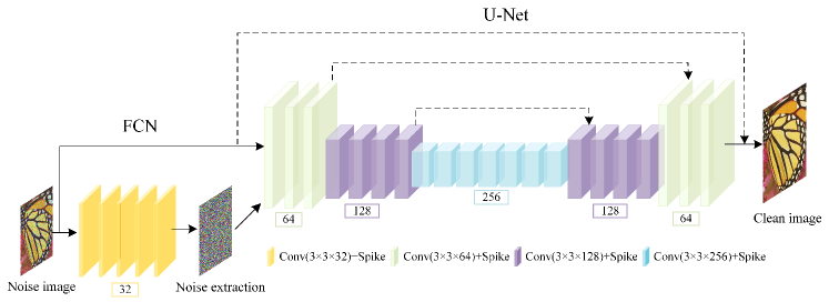
Figure 3: The architecture of the image purification neural network.

Table 1: Robustness of multi-neuron firing.

Attack	Number of neurons in an MLF unit	Accuracy
FGSM	$K=3$	79.11
	$K=2$	72.57
	$K=1$	71.67
PGD	$K=3$	45.86
	$K=2$	37.51
	$K=1$	27.45

4.1 Robust Multi-Level Firing SNNs

As described in Section 3.2, the MLF model not only enhances the expressive capabilities of neurons but also boosts the robustness of neural networks. Furthermore, it is observed that MLF also reduces the number of spike errors. Table 1 shows the experiment results on the MNIST dataset.

By performing the FGSM attack ($\epsilon$=0.2) on the pre-trained ResNet-14-based SNN model, the robustness of the multi-neuron firing is greatly improved than that of single-neuron firing. Similarly, for the PGD attack ($\epsilon$=0.2) on the model, the accuracy of $K=3$ is 18.41% higher than that of $K=1$. Meanwhile, there is no significant difference in defense performance between $K=4$ and $K=3$, which is only 2% higher, but it increases computational resource consumption. Thus, the multi-level firing SNN with $K=3$ is employed in the experiment. In addition, for compatibility with the human nervous system, we incorporate the Squeeze-and-Excitation (SE) module into SNNs. As a result, the model’s expressive capability is enhanced.

4.2 Image Purification Architecture

The imperceptible disturbance introduced by the adversarial attack can be essentially regarded as a form of noise. Therefore, the adversarial example can be considered as noise generated from the clean image following specific rules. Neuroscience’s filter theory posits that when information enters the nervous system via diverse sensory channels, it undergoes a filtering mechanism and only a portion of the information can proceed for further processing through the mechanism. Inspired by the filter theory, an image purification module is devised to reduce the noise in adversarial examples, ensuring that the data entering the functional module (classifier) closely aligns with the original data.

The architecture of the image purification network is depicted in Figure 3, which consists of a noise level estimation network and a denoising network. Firstly, the noise level estimation network is constructed based on a Fully Convolutional Network (FCN) with five full convolution layers. Through the residual learning, FCN outputs the noise level of the input image. As shown in Figure 3, the 1-st to the 5-th layers consist of 32 filters of size $3\times 3\times 3$, 32 filters of size $3\times 3\times 32$, 32 filters of size $3\times 3\times 32$, 32 filters of size $3\times 3\times 32$ and 32 filters of size $3\times 3\times 3$, respectively. Besides, the LIF non-linearity is used as an activation function. Secondly, the denoising network is built on a residual U-Net architecture. Comprehensive structural details are available in [27]. It is essential to highlight that the entire U-Net network comprises only convolutional layers, deconvolution layers, and pooling layers, without the batch normalization layers.

4.3 Proposed Loss Function

For the defense task, the primary goal is to optimize the image denoising effect with the aim of enhancing the classifier’s recognition accuracy. Typically, although $\ell_{2}$-norm regularization converges quickly, it tends to trap into local optima. In contrast, thanks to the sparsity-inducing nature that introduces non-smoothness, $\ell_{1}$-norm regularization prefers to reach more favorable minima. Thus, $\ell_{1}$-norm regularization is potentially a better choice for finding global minima [41]. For the output $\hat{\boldsymbol{x}}$ of non-blind denoising, the reconstruction loss is defined as:

$$\mathcal{L}_{\textrm{Charbonnier}}=\frac{1}{s}\cdot\sqrt{\left\|\hat{\boldsymbol{x}}-\boldsymbol{x}\right\|_{1}^{2}+c^{2}},$$ (7)

$$\mathcal{L}_{\textrm{Rec}}=\frac{\beta}{s}\cdot\sqrt{\left\|\hat{\boldsymbol{x}}-\boldsymbol{x}\right\|_{1}^{2}+c^{2}},+\frac{1-\beta}{s}\cdot\left\|\hat{\boldsymbol{x}}-\boldsymbol{x}\right\|_{2}^{2},$$

where $\boldsymbol{x}$ is the clean image, $\beta$ denotes a hyper-parameter, $s$ refers to the sample numbers, and $c$ represents a small constant (e.g. 1e-3). In this work, $\ell_{1}$-norm loss ($\mathcal{L}_{\textrm{Charbonnier}}$) is first performed to avoid prematurely falling into local optima, followed by the $\ell_{2}$-norm loss ($\mathcal{L}_{\textrm{Rec}}$) to expedite the convergence.

To leverage asymmetric sensitivity in blind denoising, we introduce an asymmetric loss for noise estimation to prevent underestimation errors in the noise level map [13]. Given the estimated noise level $\hat{\sigma}(\boldsymbol{n})$ and the ground-truth $\sigma(\boldsymbol{n})$, where $\boldsymbol{n}$ refers to the noise, the asymmetric loss on the noise level estimation network is calculated as follows:

$$\mathcal{L}_{\textrm{asym}}=\sum_{i}\left|\gamma-\mathbb{I}_{\left(\hat{\sigma}\left(n_{i}\right)-\sigma\left(n_{i}\right)\right)<0}\right|\cdot\left(\hat{\sigma}\left(n_{i}\right)-\sigma\left(n_{i}\right)\right)^{2},$$ (8)

where ${n}_{i}$ is the noise at pixel $i$. $\mathbb{I}_{e}=1$ for $e<0$ and 0 otherwise. By setting $0<\gamma<0.5$, more penalty is imposed when $\hat{\sigma}(n_{i})<\sigma(n_{i})$, enabling the model generalize well to real noise.

Furthermore, a total variation (TV) regularizer is presented to constrain the smoothness of $\hat{\sigma}(\boldsymbol{n})$, as defined in Equation 9.

$$\mathcal{L}_{\textrm{TV}}=\left\|\nabla_{h}\hat{\sigma}(\mathbf{n})\right\|_{2}^{2}+\left\|\nabla_{v}\hat{\sigma}(\mathbf{n})\right\|_{2}^{2},$$ (9)

where $\nabla_{h}(\nabla_{v})$ denotes the gradient operator along the horizontal (vertical) direction.

To sum up, the overall objective function is derived as:

$$\mathcal{L}=\mathcal{L}_{\textrm{Rec}}+\lambda_{\text{asymm}}\mathcal{L}_{\textrm{asymm}}+\lambda_{\text{TV}}\mathcal{L}_{\textrm{TV}},$$ (10)

where $\lambda_{\text{asymm}}$ and $\lambda_{\text{TV}}$ denote the tradeoff parameters for the asymmetric loss and the TV regularizer, respectively.

4.4 Image Purification Network Training

We first describe the training algorithm for the proposed image purification network. The details of the algorithm are summarized in Algorithm 1. We employ conventional attack techniques described in Section 2.1, such as FGSM, I-FGSM, PGD, and C&W, to attack the classification model, generating adversarial samples $\boldsymbol{x}_{i}^{\prime}$ and the ground-truth noise $\boldsymbol{n}_{real}$ (line 4). Then given the adversarial sample, the image purification network outputs the denosing image $\hat{\boldsymbol{x}}_{i}$ and the corresponding estimated noise $\boldsymbol{n}_{est}$ (line 5). Next, the level of the real noise $\sigma_{\boldsymbol{\theta}}(\boldsymbol{n}_{\textrm{real}})$ and the estimated noise $\sigma_{\boldsymbol{\theta}}(\boldsymbol{n}_{\textrm{est}})$ are computed, respectively (line 6). Based on above information, we calculate the loss (lines 7-10). The STBP backpropagation algorithm described in Section 3.1 is adopted to train the network. Due to the non-differentiable property of the spike activity, it is not possible to derive gradients directly, and we instead adopt the rectangular function to approximate the derivative of spike activity (line 11). Finally, the weights of the image purification network are updated (line 12).

Once the image purification network is trained with an arbitrary SNN classifier, it can be seamlessly transferred to other similar SNN classifiers. By preventing the adversarial samples from inputting directly into the SNN classifier, the accuracy is significantly enhanced.

Algorithm 1 Image Purification Network Training Algorithm

Input: $f_{\boldsymbol{\theta}}$: image purification network, $f_{\boldsymbol{c}}$: classification network, $N$: batch size, $E$: epoch number, $\epsilon$: allowed perturbation size, $\boldsymbol{n}_{\textrm{est}}$: estimated noise, $\boldsymbol{n}_{\textrm{real}}$: real noise
Output: Trained network model $\boldsymbol{\theta}$

1:for epoch $\in\{1,\ldots,E\}$ do

2:     Sample a batch $\{(\boldsymbol{x}_{i},y_{i})\}_{i=1}^{N}$ from training set

3:     for sample index $i\in\{1,\ldots,N\}$ do

4:         $\boldsymbol{x}_{i}^{\prime}$, $\boldsymbol{n}_{\textrm{real}}$ = attack$(f_{\boldsymbol{c}},\boldsymbol{x}_{i},{y}_{i},\epsilon)$

5:         $\hat{\boldsymbol{x}}_{i},\boldsymbol{n}_{\textrm{est}}=f_{\boldsymbol{\theta}}(\boldsymbol{x}_{i}^{\prime})$

6:         Compute the real noise level $\sigma_{\boldsymbol{\theta}}(\boldsymbol{n}_{\textrm{real}})$ and the estimated level $\sigma_{\boldsymbol{\theta}}(\boldsymbol{n}_{\textrm{est}})$

7:         Calculate $\mathcal{L}_{\textrm{REC}}$ using $\hat{\boldsymbol{x}}_{i}$ and $\boldsymbol{x}_{i}$ $\triangleright$ Equation 7

8:         Calculate $\mathcal{L}_{\textrm{asym}}$ and $\mathcal{L}_{\textrm{TV}}$ with $\sigma_{\boldsymbol{\theta}}(\boldsymbol{n}_{real})$ and $\sigma_{\boldsymbol{\theta}}(\boldsymbol{n}_{est})$ $\triangleright$ Equations 8 and 9

9:     end for

10:     $\mathcal{L}=\mathcal{L}_{\textrm{Rec}}++\lambda_{\text{asymm}}\mathcal{L}_{\textrm{asymm}}+\lambda_{\textrm{TV}}\mathcal{L}_{\text{TV}}$

11:     $g_{\boldsymbol{\theta}}\leftarrow\nabla_{\boldsymbol{\theta}}\mathcal{L}$

12:     $\boldsymbol{\theta}\leftarrow\operatorname{Update}(\boldsymbol{\theta},g_{\boldsymbol{\theta}})$

13:end for

4.5 Network Complexity Analysis

Time Complexity. In general, the time complexity of adversarial training comprises both the time complexity associated with generating adversarial samples and that of training the adversarial model. Specifically, the time complexity of generating adversarial samples depends on the adopted attack method and the number of samples produced during each iteration. Using the PGD attack as an illustration, the number of iterations in the PGD attack is directly proportional to the time complexity of generating adversarial samples. After obtaining adversarial samples, the model is trained using both the original and adversarial samples. As demonstrated in [14], the training time complexity is estimated as:

$$\textrm{Time}\sim\mathcal{O}(\sum_{l=1}^{D}M_{l}^{2}\cdot K_{l}^{2}\cdot C_{l-1}\cdot C_{l}),$$ (11)

where $D$ is the number of convolutional layers. $M_{l}$ and $K_{l}$ denote the spatial size (length) of the output feature map and the kernel in $l$-th layer. Besides, $C_{l}$ refers to the number of kernels in the $l$-th layer. Accordingly, $C_{l-1}$ is also known as the number of input channels in the $l$-th layer.

Similarly, the time complexity of the image purification network also contains the above two components. However, the advantage of our proposed network is that the training time complexity remains constant and does not vary with specific tasks. Additionally, our network requires fewer attack iterations to produce adversarial samples.

Space Complexity. The space complexity of a neural network is usually measured by its parameters, which can be expressed by the following formula:

$$\textrm{Space}\sim\mathcal{O}(\sum_{l=1}^{D}K_{l}^{2}\cdot C_{l-1}\cdot C_{l}+\sum_{l=1}^{D}M_{l}^{2}\cdot C_{l}).$$ (12)

Since the parameter number of the model is independent of the size of the input data, the space complexity of the proposed denoising method and adversarial training depends on the number of parameters in the image purification network and the classification model, respectively. For different tasks, adversarial training usually employs different classification networks. As the task’s complexity grows, the neural network tends to become deeper, leading to an augmentation of the number of parameters. Conversely, the parameter number of the image purification network remains consistent, making it more advantageous in complex tasks. In fact, the total number of parameters of our proposed image purification network is only 4 million. In contrast, commonly employed models in computer vision typically exhibit parameter numbers in the tens or even hundreds of millions, which highlights the potential resource savings in our image purification approach.

5 Experimental Results

5.1 Experiment Setup

Platform. The implementation of our methodology is in Python with the Pytorch [26], and we execute it on a platform with Intel Xeon Gold 6248R CPU and Nvidia A100-PCIE-40GB GPU.

Dataset. We conduct experiments on multiple datasets, including CIFAR-10/100 [19] and Street View House Number (SVHN) [23]. The CIFAR-10 and CIFAR-100 datasets consist of 10 and 100 categories, respectively. Each dataset comprises 60,000 color images with size of $32\times 32$, with 50,000 images for training and 10,000 for validation. The SVHN dataset, a real-world image dataset, is divided into three parts: the training set, the testing set, and an extra set. In the experiment, only the training and test sets are used, where the training and test set contain 73,257 and 26,032 labeled digital images, respectively.

SNN Model. Multi-level firing SNNs based on Squeeze-and-Excitation Network (SENet18-SNN) [16] is adopted to verify the effectiveness of our methodology.

Adversarial Attack Setting. To evaluate the adversarial robustness of our proposed method, we perform experiments using various attack strategies, including the FGSM [12], I-FGSM [32], MI-FGSM [8], PGD [22], CW [3], APGD and AutoAttack [5]. The size of the allowed adversarial perturbation $\epsilon$ is set to 8/255 for FGSM, I-FGSM, MI-FGSM, PGD, and APGD. Besides, the number of iterations for PGD, I-FGSM, and MI-FGSM are set to 7 with a step size of 2/255. For CW attack, the learning rate is set to 0.01 with 50 steps.

Table 2: Robustness comparison with the SOTA mechanisms on CIFAR-10, CIFAR-100 and SVHN datasets. Adversarial training is labeled as “Adv”, Online label smoothing as “OLS”.

Dataset	Method	Clean Accuracy	Gaussain	FGSM	I-FGSM	MI-FGSM	PGD	CW
SVHN	Conversion-SNN [24]	96.56	$-$	56.66	$-$	$-$	36.02	$-$
	Ours	89.98	90.88	82.96	89.97	84.46	88.35	90.75
	Ours + OLS	89.94	91.21	84.64	89.14	85.05	90.13	89.95
CIFAR-10	HIRE-SNN [20]	87.50	$-$	38.00	$-$	$-$	9.10	$-$
	RAT-SNN [7]	90.74	$-$	45.23	$-$	$-$	21.16	$-$
	CARENet[40]	84.10	58.70	71.10	$-$	$-$	70.70	56.10
	HoSNN(without Adv) [11]	91.62	$-$	72.62	64.46	$-$	54.19	$-$
	HoSNN(with Adv) [11]	90.30	$-$	75.22	71.21	$-$	68.99	$-$
	Ours	89.05	79.05	75.63	70.71	66.43	74.16	83.69
	Ours + OLS	88.43	80.74	79.14	83.80	82.04	83.23	83.03
CIFAR-100	HIRE-SNN [20]	65.10	$-$	22.00	$-$	$-$	7.50	$-$
	RAT-SNN [7]	70.89	$-$	25.86	$-$	$-$	10.38	$-$
	HoSNN(without Adv) [11]	70.14	$-$	9.30	1.52	$-$	0.55	$-$
	HoSNN(with Adv) [11]	65.37	$-$	27.18	22.58	$-$	18.47	$-$
	Ours	66.98	41.05	43.14	42.89	37.52	46.04	56.31
	Ours + OLS	66.84	43.81	46.57	46.74	41.97	48.78	56.30

Training Strategy. First, the SNN classifier is trained utilizing a state-of-the-art strategy. For the SVHN dataset, the classifier is trained for 50 epochs using a batch size of 512 through SGD with the learning rate of 0.01. We employ a piecewise decay learning rate scheduler with a decay factor of 0.1 at the 25-th and 35-th epochs. For CIFAR-10/100 dataset, we train the SNN classifier for 150 epochs with a batch size of 256 via SGD, and the learning rate is set to 0.1. The piecewise decay learning rate scheduler is also performed with a decay factor of 0.1 at 80 and 120 epochs. Throughout the training process, the timestep is set to 4 and the neuron firing threshold vector $\boldsymbol{V}_{th}$ is configured as [0.6, 1.6, 2.6]. In order to assess the impact of the proposed image purification network in collaboration with other defense methods, we further train an SNN classifier using the Online Label Smoothing (OLS) [36] strategy. The hyperparameter settings remain consistent with those of the model without OLS.

Concerning the image purification network, we conduct the training for 200 epochs with a batch size of 128 using the Adam optimizer, where the learning rate is configured as $1\times e^{-4}$. In the experiment, we find that the adversarial samples generated by single-step attacks and multi-step iteration attacks, respectively, do not significantly change the defense performance of the image purification network. Thus, considering the training overhead, we apply the FGSM ($\epsilon=16/255$) to attack the SNN classifier.

5.2 Comparison with State of the Arts

5.2.1 Noise Robustness

We first verify the robustness of the proposed image purification network against the noise. In the experiment, a Gaussian noise with a noise level 20 is introduced in the dataset. Table 2 summarizes the experimental results. As shown in the table, with the image purification module, the classification accuracy reaches 90.88% on SVHN, 79.05% on CIFAR-10 and 41.05% on CIFAR-100.

5.2.2 White-box Robustness

We then demonstrate the effectiveness of the proposed image purification network against the white-box attacks. The experimental results are listed in Table 2. The better results are emphasized in bold in the table. For the CIFAR-10/100 datasets, our method achieves greater robustness compared to SOTA works under different types of white-box attacks. For example, for the CIFAR-10 dataset, compared with the HoSNN joint adversarial training method [11], the accuracy of the proposed image purification trained combined with the OLS defense method is increased by 8.58% under FGSM attacks, 12.02% under I-FGSM attacks, and 14.04% under PGD attacks. Similarly, for the CIFAR-100 dataset, our methodology improves the accuracy by 19.39%, 24.16%, and 30.31% under FGSM, I-FGSM, and PGD attacks, respectively. Besides, the proposed method achieves a robust accuracy of 56.30% and 41.97% under CW and MI-FGSM attacks, respectively. The results demonstrate that our proposed image purification network model performs well against white-box attacks.

Table 3: Robust accuracy(%) of black-box attacks on CIFAR-10.

Surrogate model	Attack	Ours	OLS
WideResNet16-8-SNN	FGSM	79.86	45.89
	PGD5	80.95	35.06
	PGD10	78.96	22.67
	PGD20	78.85	19.48
ResNet20-SNN	FGSM	79.99	55.78
	PGD5	80.96	43.02
	PGD10	79.29	28.04
	PGD20	79.36	22.10

Figure 4: Time comparison of our method with adversarial training.

(a) CIFAR-100

(b) CIFAR-100

(c) SVHN

(d) SVHN

Figure 5: The evaluation of the stronger PGD attack (step size: 2/255) with SENet18-SNN on CIFAR-100 and SVHN. No defense is labeled as “Baseline”, Online label smoothing as “OLS”, Proposed Image purification model as “Ours”.

5.2.3 Black-box Robustness

We further validate the defense performance of our proposed methodology against transferable black-box attacks. Adversarial samples for black-box attacks are created by attacking a pretrained surrogate model on the original training set. In the experiment, we assess black-box robustness using WideResNet16-8-SNN and ResNet20-SNN surrogate models trained on the CIFAR-10 dataset with 100 epochs. The adopted attacking methods include FGSM, PGD⁵, PGD¹⁰, and PGD²⁰ with $\epsilon=8/255$. Table 3 lists the results averaged over three independent experiments. As illustrated in the table, although soft labeling methods like OLS demonstrate robustness against white-box attacks, the accuracy is significantly reduced under the black-box scenario. In contrast, our method maintains accuracy within an acceptable range in black-box attacks, with an average improvement of over 40% compared to the OLS method.

5.2.4 Time Efficiency

In the end, we conduct experiment to verify the time efficiency of the proposed methodology. In our method, after the image purification network is trained, we directly establish a sequential connection by linking this network ahead of the multi-level SNN classifier. In the comparison experiment, the SNN classifier is trained with adversarial training. As illustrated in Figure 4, in contrast to adversarial training, the proposed image purification method achieves an average reduction of 93.9% in training time across all three datasets. The reason is that the training time complexity of the proposed model remains constant and does not vary with specific tasks. Additionally, our network requires fewer attack iterations to produce adversarial samples.

The above experimental results demonstrate the proposed SNN-based image purification network provides superior defense effectiveness and significantly reduces training time consumption. In addition, the proposed network trained with any classifier can be easily transferred to other similar classifiers for defense. For example, the image purification network trained with SENet18-SNN can be migrated to ResNet20-SNN, and the accuracy under various attacks is similar to the results in Table 2.

5.3 Evaluate with Stronger Attacks

We further assess the performance of our algorithm under more challenging attacks. The experiment is conducted on SVHN and CIFAR-100, as depicted in Figure 5. We mainly consider two scenarios, involving the PGD attack with more steps and larger maximum perturbation sizes $\epsilon$. Specifically, we consider the attacking scenario of PGD⁵, $\ldots$, PGD⁵⁰, and $\epsilon\in[1/255,16/255]$. In contrast to adversarial training, where accuracy tends to decline with more steps [35], our image purification defense method consistently maintains high accuracy even under PGD⁵⁰, as illustrated in Figure 5a and Figure 5c. For example, for CIFAR-100 under PGD attack with $\epsilon=8/255$ and steps 5 to 50, the accuracy of our method remains above 40%. Meanwhile, for SVHN, the accuracy of our method reaches above 70% with $\epsilon=16/255$ and steps 5 to 50. Considering the PGD size, our method still exhibits robust performance under larger perturbation sizes, as illustrated in Figure 5b and Figure 5d. On CIFAR-100, our method achieves 59.25% and 44.64% accuracy under PGD attack with $\epsilon=1/255$ and $\epsilon=16/255$, respectively, where the accuracy drop is only 14.61%. Similarly, on SVHN, the accuracy drop of our method is only 7.95% (90.09% $\to$ 82.14%).

In addition, as illustrated in Figure 5b and Figure 5d, there is a notable decrease in robustness accuracy when the maximum perturbation is set to 16/255. This phenomenon can be attributed to the intrinsic sensitivity of non-blind denoising networks [39], which generally respond unfavorably to underestimating noise levels but exhibit effective performance when noise levels are overestimated. Specifically, if the noise level extracted by the image purification network is underestimated, the denoising result will be less favorable. Thus, we prefer to set a higher perturbation level in generating adversarial samples to enhance our our model against stronger attacks.

We have further presented the performance of our methodology under the latest attack benchmarks in Table 4. Column “APGD_ce” represents the APGD attack with the cross-entropy loss, while columns “AutoAttack” and “BPDA+EOT” denote the ensemble attack and adaptive attack, respectively. As shown in the table, compared with the current SOTA defense works, our method achieves accuracy improvements of 57.99%, 19.38%, and 29.95% under APGD_ce attack on SVHN, CIFAR-10 and CIFAR-100 datasets. Besides, the defense performance trends are the same under AutoAttack and BPDA+EOT attacks. The results demonstrate that the proposed network model can generalize to other adversarial attacks not in training and against more prominent ones.

Table 4: The evaluation of the advanced attacks. All attacks are estimated under $l_{\infty}$-norm bounded with $\epsilon$ = 8/255.

Dataset	Method	APGDce	AutoAttack	BPDA20+EOT
SVHN	Conversion-SNN [24]	31.04	27.65	$-$
	Ours	89.03	90.58	88.75
CIFAR-10	Conversion-SNN [24]	51.65	45.05	$-$
	CARENet(without Adv) [40]	$-$	46.10	$-$
	CARENet(with Adv) [40]	$-$	47.20	$-$
	Ours	71.03	71.48	69.48
CIFAR-100	Conversion-SNN [24]	13.26	11.04	$-$
	Ours	43.21	43.07	40.76

6 Conclusion

In this paper, we have proposed an end-to-end image purification network and a robust SNNs structure aimed at defending against adversarial examples. Through the pre-processing of input images the image purification module effectively mitigates noise, thereby minimizing the discrepancy between the adversarial sample and the clean image. Significantly, our method outperforms defense techniques such as adversarial training in terms of defense effectiveness and time efficiency. We believe this work will stimulate more research on the adversarial security design of SNNs.

References

- Auge et al. [2021] D. Auge, J. Hille, E. Mueller, and A. Knoll. A survey of encoding techniques for signal processing in spiking neural networks. Neural Processing Letters, 53(6):4693–4710, 2021.
- Bi et al. [2023] Y. Bi, Q. Xu, H. Geng, S. Chen, and Y. Kang. AD2VNCS: Adversarial defense and device variation-tolerance in memristive crossbar-based neuromorphic computing systems. ACM Transactions on Design Automation of Electronic Systems (TODAES), 29(1):1–9, 2023.
- Carlini and Wagner [2017] N. Carlini and D. Wagner. Towards evaluating the robustness of neural networks. In IEEE Symposium on Security and Privacy (SP), pages 39–57, 2017.
- Chorowski et al. [2015] J. Chorowski, D. Bahdanau, D. Serdyuk, K. Cho, and Y. Bengio. Attention-based models for speech recognition. In Conference on Neural Information Processing Systems (NIPS), pages 577–585, 2015.
- Croce and Hein [2020] F. Croce and M. Hein. Reliable evaluation of adversarial robustness with an ensemble of diverse parameter-free attacks. In International Conference on Machine Learning (ICML), pages 2206–2216, 2020.
- Davies et al. [2018] M. Davies, N. Srinivasa, T.-H. Lin, G. Chinya, Y. Cao, S. H. Choday, G. Dimou, P. Joshi, N. Imam, S. Jain, et al. Loihi: A neuromorphic manycore processor with on-chip learning. IEEE Micro, 38(1):82–99, 2018.
- Ding et al. [2022] J. Ding, T. Bu, Z. Yu, T. Huang, and J. Liu. SNN-RAT: Robustness-enhanced spiking neural network through regularized adversarial training. In Conference on Neural Information Processing Systems (NIPS), pages 24780–24793, 2022.
- Dong et al. [2018] Y. Dong, F. Liao, T. Pang, H. Su, J. Zhu, X. Hu, and J. Li. Boosting adversarial attacks with momentum. In IEEE Conference on Computer Vision and Pattern Recognition (CVPR), pages 9185–9193, 2018.
- Feng et al. [2022] L. Feng, Q. Liu, H. Tang, D. Ma, and G. Pan. Multi-level firing with spiking DS-ResNet: Enabling better and deeper directly-trained spiking neural networks. arXiv preprint arXiv:2210.06386, 2022.
- Garg et al. [2021] I. Garg, S. S. Chowdhury, and K. Roy. DCT-SNN: Using DCT to distribute spatial information over time for low-latency spiking neural networks. In IEEE International Conference on Computer Vision (ICCV), pages 4671–4680, 2021.
- Geng and Li [2023] H. Geng and P. Li. HoSNN: Adversarially-robust homeostatic spiking neural networks with adaptive firing thresholds. arXiv preprint arXiv:2308.10373, 2023.
- Goodfellow et al. [2014] I. J. Goodfellow, J. Shlens, and C. Szegedy. Explaining and harnessing adversarial examples. arXiv preprint arXiv:1412.6572, 2014.
- Guo et al. [2019] S. Guo, Z. Yan, K. Zhang, W. Zuo, and L. Zhang. Toward convolutional blind denoising of real photographs. In IEEE Conference on Computer Vision and Pattern Recognition (CVPR), pages 1712–1722, 2019.
- He and Sun [2015] K. He and J. Sun. Convolutional neural networks at constrained time cost. In IEEE Conference on Computer Vision and Pattern Recognition (CVPR), pages 5353–5360, 2015.
- He et al. [2016] K. He, X. Zhang, S. Ren, and J. Sun. Deep residual learning for image recognition. In IEEE Conference on Computer Vision and Pattern Recognition (CVPR), pages 770–778, 2016.
- Hu et al. [2018] J. Hu, L. Shen, and G. Sun. Squeeze-and-excitation networks. In IEEE Conference on Computer Vision and Pattern Recognition (CVPR), pages 7132–7141, 2018.
- Kim and Panda [2021] Y. Kim and P. Panda. Revisiting batch normalization for training low-latency deep spiking neural networks from scratch. Frontiers in neuroscience, 15:773954, 2021.
- Kim et al. [2023] Y. Kim, Y. Li, H. Park, Y. Venkatesha, A. Hambitzer, and P. Panda. Exploring temporal information dynamics in spiking neural networks. In AAAI Conference on Artificial Intelligence, pages 8308–8316, 2023.
- Krizhevsky [2009] A. Krizhevsky. Learning multiple layers of features from tiny images. Master’s thesis, University of Toronto, 2009.
- Kundu et al. [2021] S. Kundu, M. Pedram, and P. A. Beerel. HIRE-SNN: Harnessing the inherent robustness of energy-efficient deep spiking neural networks by training with crafted input noise. In IEEE International Conference on Computer Vision (ICCV), pages 5209–5218, 2021.
- Liu et al. [2022] Y. Liu, Y. Cheng, L. Gao, X. Liu, Q. Zhang, and J. Song. Practical evaluation of adversarial robustness via adaptive auto attack. In IEEE Conference on Computer Vision and Pattern Recognition (CVPR), pages 15105–15114, 2022.
- Madry et al. [2017] A. Madry, A. Makelov, L. Schmidt, D. Tsipras, and A. Vladu. Towards deep learning models resistant to adversarial attacks. arXiv preprint arXiv:1706.06083, 2017.
- Netzer et al. [2011] Y. Netzer, T. Wang, A. Coates, A. Bissacco, B. Wu, and A. Y. Ng. Reading digits in natural images with unsupervised feature learning. In NIPS Workshop on Deep Learning and Unsupervised Feature Learning, pages 1–9, 2011.
- Özdenizci and Legenstein [2023] O. Özdenizci and R. Legenstein. Adversarially robust spiking neural networks through conversion. arXiv preprint arXiv:2311.09266, 2023.
- Papernot et al. [2016] N. Papernot, P. McDaniel, X. Wu, S. Jha, and A. Swami. Distillation as a defense to adversarial perturbations against deep neural networks. In IEEE Symposium on Security and Privacy (SP), pages 582–597, 2016.
- Paszke et al. [2017] A. Paszke, S. Gross, S. Chintala, G. Chanan, E. Yang, Z. DeVito, et al. Automatic differentiation in PyTorch. In NIPS Workshop, 2017.
- Ronneberger et al. [2015] O. Ronneberger, P. Fischer, and T. Brox. U-Net: Convolutional networks for biomedical image segmentation. In Medical Image Computing and Computer-Assisted Intervention (MICCAI), 2015.
- Ross and Doshi-Velez [2018] A. Ross and F. Doshi-Velez. Improving the adversarial robustness and interpretability of deep neural networks by regularizing their input gradients. In Proceedings of the AAAI conference on artificial intelligence, volume 32, 2018.
- Selvaraju et al. [2017] R. R. Selvaraju, M. Cogswell, A. Das, R. Vedantam, D. Parikh, and D. Batra. Grad-CAM: Visual explanations from deep networks via gradient-based localization. In IEEE International Conference on Computer Vision (ICCV), pages 618–626, 2017.
- Sengupta et al. [2019] A. Sengupta, Y. Ye, R. Wang, C. Liu, and K. Roy. Going deeper in spiking neural networks: VGG and residual architectures. Frontiers in neuroscience, 13:95, 2019.
- Sharmin et al. [2020] S. Sharmin, N. Rathi, P. Panda, and K. Roy. Inherent adversarial robustness of deep spiking neural networks: Effects of discrete input encoding and non-linear activations. In European Conference on Computer Vision (ECCV), pages 399–414, 2020.
- Tramèr et al. [2017] F. Tramèr, A. Kurakin, N. Papernot, I. Goodfellow, D. Boneh, and P. McDaniel. Ensemble adversarial training: Attacks and defenses. arXiv preprint arXiv:1705.07204, 2017.
- Vaswani et al. [2017] A. Vaswani, N. Shazeer, N. Parmar, J. Uszkoreit, L. Jones, A. N. Gomez, Ł. Kaiser, and I. Polosukhin. Attention is all you need. In Conference on Neural Information Processing Systems (NIPS), pages 6000–6010, 2017.
- Wu et al. [2018] Y. Wu, L. Deng, G. Li, J. Zhu, and L. Shi. Spatio-temporal backpropagation for training high-performance spiking neural networks. Frontiers in neuroscience, 12:331, 2018.
- Xie et al. [2019] C. Xie, Y. Wu, L. v. d. Maaten, A. L. Yuille, and K. He. Feature denoising for improving adversarial robustness. In IEEE Conference on Computer Vision and Pattern Recognition (CVPR), pages 501–509, 2019.
- Zhang et al. [2021] C.-B. Zhang, P.-T. Jiang, Q. Hou, Y. Wei, Q. Han, Z. Li, and M.-M. Cheng. Delving deep into label smoothing. IEEE Transactions on Image Processing, 30:5984–5996, 2021.
- Zhang et al. [2019] H. Zhang, Y. Yu, J. Jiao, E. Xing, L. El Ghaoui, and M. Jordan. Theoretically principled trade-off between robustness and accuracy. In International Conference on Machine Learning (ICML), pages 7472–7482, 2019.
- Zhang et al. [2023a] H. Zhang, J. Cheng, J. Zhang, H. Liu, and Z. Wei. A regularization perspective based theoretical analysis for adversarial robustness of deep spiking neural networks. Neural Networks, 165:164–174, 2023a.
- Zhang et al. [2018] K. Zhang, W. Zuo, and L. Zhang. FFDNet: Toward a fast and flexible solution for CNN-based image denoising. IEEE Transactions on Image Processing, 27(9):4608–4622, 2018.
- Zhang et al. [2023b] Y. Zhang, C. Chen, D. Shen, M. Wang, and B. Wang. Take CARE: Improving inherent robustness of spiking neural networks with channel-wise activation recalibration module. In IEEE International Conference on Data Mining (ICDM), pages 828–837, 2023b.
- Zhao et al. [2016] H. Zhao, O. Gallo, I. Frosio, and J. Kautz. Loss functions for image restoration with neural networks. IEEE Transactions on Computational Imaging, 3(1):47–57, 2016.