On the equivalence of the semiclassical theory and the response theory

Abstract

It is long believed that the response theory can give quantum correction (or interband coherent effects) to the semiclassical theory, while both formulations essentially are perturbatively solving the time-dependent Schödinger equation in a periodic potential probed by the electric field within the independent-particle approximation. In this work, by extending the semiclassical theory under a uniform electric field to the nonlinear AC regime, we show explicitly that up to the second order of electric field, the AC semiclassical theory gives exactly the same results as the response theory in the absence of relaxation. Remarkably, this equivalence can be expected even in DC limit when the zero-frequency divergence is regulated on the same footing. Particularly, at the linear order of the electric field, we show that both formulations deliver the same Drude current, intrinsic anomalous Hall current, and the displacement current, where the last one arising from the time variation of the first-order positional shift can only appear in AC transport and is usually overlooked. Furthermore, at the second order of the electric field, we show that all the well-known transport effects, including the nonlinear Drude and Hall effects (that can be driven by the Berry curvature dipole or/and quantum metric dipole) can be derived by both formulations. Additionally, we show that the nonlinear displacement current due to the time variation of the second-order positional shift and the nonlinear intrinsic Ohmic current due to the second-order energy correction (which is determined by the first-order positional shift) in AC semiclassical theory can also be obtained by response theory. As a consequence of this equivalence, (i) we suggest that the energy used in the equilibrium Fermi distribution particularly in the semiclassical theory is the unperturbed band energy; (ii) more importantly, we conclude that the semiclassical theory does not ignore any interband coherent effects compared to the response theory and the distinction between them is fundamentally rooted in the way to introduce the relaxation; (iii) last but not least, the scheme of introducing relaxation used in response theory usually by modifying the quantum Liouville equation need to be reconsidered.

I Introduction

Understanding the response or transport behaviors of Bloch electrons in crystalline solids probed by the electromagnetic field is one of the oldest but still most important themes in condensed matter physics Mermin , which may be traced back to the phenomenological Drude model for metal with a finite Fermi surface. Along this approach, by treating the Bloch electron as a wavepacket which satisfies the Schrödinger equation, the semiclassical equations of motion Niu1996 ; Niu1999 ; Xiao2010 ; footnote1 ($e=\hbar=1$)

$$\dot{\bm{r}} =-\dot{\bm{k}}\times\bm{\Omega}+\partial_{\bm{k}}\epsilon,$$ (1)

$$\dot{\bm{k}} =-\dot{\bm{r}}\times\bm{B}-\bm{E},$$ (2)

are proposed to evaluate the velocity for the position center $\bm{r}$ of the wavepacket in phase space (Throughout this work, we will focus on the responses that driven by the electric field although Eq.(2) in general includes the magnetic field). Furthermore, by solving the Boltzmann equation for the nonequilibrium distribution function $\bar{f}_{n}$ for the $n$th band,

$$\bm{E}\cdot\nabla_{\bm{k}}\bar{f}_{n}-\partial_{t}\bar{f}_{n}=(\bar{f}_{n}-f_{n}^{(0)})/\tau,$$ (3)

the current at linear/nonlinear regime can be calculated BCD ; GaoY2014 ; GaoY2019 ; BPT ; XiaoCnc ; E0Ew1 ; E0Ew2 . In Eq.(3), the scattering is introduced by adopting the relaxation time ($\tau$) approximation. Importantly, the linear/nonlinear current conductivity tensors usually are expressed by the quantum Bloch wavefunction and thereby the quantum geometry QuantumGeometry ; QuantumGeometry1 ; QuantumGeometry2 and the topological properties topology ; Nagaosa2017 ; JEMoore2017 encoded in Bloch states can be read out from the detected current, particularly by manipulating the symmetry that bridges the quantum geometric quantities and the conductivity tensors. In fact, Eqs.(1-3), especially when combining with the well-developed first-principles material calculations Yanfirst , offers one of the most successful theoretical methods to explain the exotic linear/nonlinear transport experiments, such as the intrinsic anomalous Hall effect FZ2003 ; YaoYG2004 ; Nagaosa2010 in ferromagnetic metals and the extrinsic nonlinear anomalous Hall effect observed in nonmagnetic metallic quantum materials BCDexp1 ; BCDexp2 ; BCDexp3 , where the Berry curvature $\bm{\Omega}$ plays an essential role. Recently, based on the second-order semiclassical theory GaoY2014 , one further realizes that the band-geometric quantity—quantum metric, which in conjunction with the Berry curvature constitutes the quantum geometric tensor, also plays a pivotal role particularly in observing the intrinsic second-order nonlinear anomalous Hall effect intrinsic20211 ; intrinsic20212 ; XuSY2023 ; Wang2023 ; MNHE1 ; MNHE2 . These progresses initiate the quantum geometric physics QuantumGeometry in condensed matter systems, where the conventional wisdom that the response of a solid to a weak electric and magnetic fields is fully determined by the band dispersion is shifting.

Compared to the transport in metal, the response properties of Bloch electrons in insulators with a vanishing Fermi surface are very often explored by irradiating light, which may be traced back to the phenomenological Lorentz model Lorentz based on the oscillator model of dielectric solids. Up to date, the more advanced and mature technique used to tackle with the same problem is the response theory JEMoore2019 ; Sipe1995 ; Sipe2000 , where the valence electrons by absorbing a photon to form a resonant conducting current can be well captured. Also by combining with the well-developed first-principles material calculations, the expressions derived by response theory can also be used to evaluate the photocurrent in realistic materials Rappe2012 ; Yan2019 ; Wanghua2020 ; Rappe2023 . In particular, the fundamental equation that is solved to obtain the linear and nonlinear photocurrent conductivities is the quantum Liouville equation for the non-equilibrium density matrix $\rho$ JEMoore2019 ; Sipe1995 ; Sipe2000 ,

$$i\partial_{t}\rho=[H,\rho],$$ (4)

where $H=H_{0}+H_{1}$ is the total Hamiltonian. To be specific, $H_{0}$ is the solved periodic Hamiltonian with $H_{0}|u_{n}\rangle=\epsilon_{n}|u_{n}\rangle$, where $u_{n}$ is the periodic part of Bloch states and $\epsilon_{n}$ is the band energy for the $n$th band. In addition, $H_{1}=\bm{E}(t)\cdot\bm{r}$ is the perturbed electric field at length gauge.

Similar to the semiclassical theory, there are a few of transport experiments relax ; Hualingzeng that can be well explained by theoretical calculations based on response theory, such as the shift and injection photocurrent at the second order of optical electric field. Importantly, these exotic responses are also believed to be intimately related to the quantum geometry of Bloch electrons MaQlight ; JTsong .

Although having different starting points, the semiclassical theory and the response theory have been shown to be complementary in many aspects. For example, the semiclassical limit ($\omega\rightarrow 0$ with $\omega$ the driving frequency) of nonlinear optical responses obtained within velocity gauge JEMoore2019 usually are needed to be benchmarked by Eq.(1-2) in the absence of magnetic field $\bm{B}$, particularly to reveal the effect of Berry phase Xiao2010 . In addition, the semiclassical formulation for the extrinsic second-order nonlinear anomalous Hall effect has been proposed to rectify the high-frequency Terahertz spectrum Terahertz ; Terahertz1 . In fact, all the semiclassical (charge) response relations particularly under the electric field, such as the linear/nonlinear anomalous Hall effect, can also be reproduced with the response theory, but there are some response relations based on the response theory in DC transport regime has not been fully accessed by the semiclassical theory Yanase2020 ; Yanunify ; CulcerPRBL ; GangSu2022 ; intrinsicThird , such as the intrinsic second-order nonlinear intrinsic Ohmic current CulcerPRBL ; GangSu2022 . This brought up a controversial issue as whether two formulations can give the same result.

In addition, the recent interplay between the semiclassical theory and the response theory at nonlinear regimes poses two challenges that can make the two formulations not equivalent. It is known that the advantage of the semi-classical theory comes from its intuitive physical picture such as Berry curvature, while this approach becomes conceptually rather involved in treating the nonlinear effect. For instance in dealing with the nonlinear effect, the external fields give corrections to the band energy and wave function of the underlying system which in turn may influence various quantities such as the Fermi distribution function and the Berry curvature. Specifically, in the second order semi-classical theory when magnetic field is absent, the DC current density has been expressed asGaoY2014

$$\bm{J}=\sum_{n}\int_{k}f_{n}[\bar{\bm{v}}_{n}+\bm{E}\times\bar{\bm{\Omega}}_{n}]$$ (5)

where $\bar{\bm{v}}_{n}=\nabla_{k}{\bar{\epsilon}}_{n}$ is the field dependent band velocity, ${\bar{\epsilon}}_{n}$ is the field dependent energy, and ${\bar{\bf\Omega}}_{n}$ is the field dependent Berry curvature. It is not fully justified whether the equilibrium Fermi distribution function $f_{n}$ should be affected by external fields, i.e., whether $f_{n}$ in Eq.(5) should be written as $f({\bar{\epsilon}}_{n})$BPT ; Y-Gao2019 or $f(\epsilon_{n})$ ($\epsilon_{n}$ is the unperturbed band energy). This is the first challenge to cope with.

The calculation of response theory, on the other hand, is straightforward although the algebra can be complicated. In addition, the inclusion of relaxation into the response theory has been proposed phenomenologically by modifying Eq.(4)Mikhailov ; Peres ,

$$i\partial_{t}\rho=[H,\rho]-\frac{i}{\tau}(\rho-\rho^{(0)})$$ (6)

where $\rho^{(0)}$ is the equilibrium density matrix and $\tau$ is the relaxation time. Although Eq.(6) has been used in many studies Sodemann2019 ; HWXu2021 ; Culcer2022 , its relation to the Boltzmann equation used in the semi-classical theory is not clear. Since in the DC case the occurrence of the relaxation is mathematically originated from the diverging conductivity, how to regularize the divergence by introducing phenomenological scattering mechanism is another challenge. More importantly, although the semi-classical theory and the response theory gives the same result in the linear regime Luttinger1958 ; Sinitsyn2007PRB ; Sinitsyn2007 , a comprehensive discussion on the relationship between these two approaches in the nonlinear regime especially when the external field is time-dependent (i.e., in ac regime) need more efforts Yanunify ; XiaoC2019PRB , which is also urgent to gain a complete understanding of the relationship between two approaches.

In this work, by extending the conventional semiclassical theory under a uniform electric field to the AC regime, we show that up to the second order of electric field, the AC semiclassical theory is equivalent to the response theory in clean limit and this equivalence can be expected even in DC limit when the zero-frequency divergence is properly regulated by introducing the scattering mechanism. In particular, at the linear order of the electric field, we show that both formulations can give the same linear Drude current, intrinsic anomalous Hall current, and the displacement current, in which the last one arising from the time variation of the first-order positional shift can only be driven by a AC field and is usually overlooked even in AC transport. Furthermore, at the second order of the electric field, we show that all the well-known transport effects, including the nonlinear Drude current, the nonlinear Hall current that driven by the Berry curvature dipole and quantum metric dipole, respectively, can be derived with both formulations. In addition, we find that the nonlinear displacement current due to the second-order position shift and the nonlinear intrinsic current due to the band energy correction (which in fact is determined by the first-order positional shift) in AC semiclassical theory can also be evaluated with the response theory. Finally, based on the equivalence, we conclude that the energy used in the equilibrium Fermi distribution should not contain the correction due to the electric field particularly in the clean limit. We also conclude that the distinctions between both formulation are rooted from the way to introduce the relaxation, which may lead to additional quantum corrected nonlinear currents beyond the semiclassical theory. However, Eq.(6) is ruled out since it gives a linear extrinsic Hall effect in time-reversal invariant systems which contradicts with experimental findings. By regularizing the DC diverging conductivity, a scheme is proposed to introduce the relaxation in the response theory.

II AC semiclassical theory

In this section, we extend the calculation of DC semiclassical theory under a uniform electric field to AC regime, particularly accurate up to the second order of the applied electric field. In detail, we construct the wavepacket accurate up to the second order of the AC electric field and then evaluate the position center for the wavepacket, where the key expressions for the positional shift up to the second order of the AC electric field are obtained. In addition, we derive the equations of motions for the wavepacket centers (including momentum and position) and find that the AC semiclassical velocity compared to the DC one contains an additional contribution, which is solely decided by the time variation of positional shift and does not show up in DC transport. Finally, we estimate the wavepacket energy accurate up to the second order of the AC electric field, where the second-order energy correction can also be expressed by the first-order positional shift, like the DC semiclassical theory.

II.1 The wavepacket accurate up to the second order

Following the spirit of the semiclassical wavepacket theory Xiao2010 ; GaoY2014 , we focus on the $n$th band to construct the wavepacket as follows ($e=\hbar=1$):

$$|W\rangle=\int_{\bm{p}}e^{i\bm{p}\cdot\bm{r}}\left(C_{n}(\bm{p})|u_{n}\rangle+\sum_{l\neq n}\bar{C}_{l}(\bm{p})|u_{l}\rangle\right),$$ (7)

where $\int_{\bm{p}}\equiv\int d\bm{p}/(2\pi)^{d}$ with $d$ the system dimension, $|u_{n}\rangle\equiv|u_{n}(\bm{p})\rangle$ is periodic part of the Bloch state, $C_{n}(\bm{p})$ is the zero-order amplitude and $\bar{C}_{l}(\bm{p})$ stands for the correction (indicated with a bar above $C_{l}$) induced by the external electric field (Throughout this work, we will only consider the electric field). Here we assume that Xiao2010

$$|C_{n}(\bm{p})|^{2}=\delta(\bm{p}-\bm{p}_{c})$$ (8)

with $\bm{p}_{c}$ the momentum center to normalize the wavepacket up to the first order Xiao2010 . Note that Eq.(8) is useful in evaluating various quantities related to the wavepacket.

As the superposition of Bloch states, the wavepacket obeys the time-dependent Schrödinger equation

$$i\partial_{t}|W\rangle=H|W\rangle,$$ (9)

where $\partial_{t}=\partial/\partial t$, $H=H_{0}+H_{1}$ with $H_{0}$ the periodic crystal Hamiltonian, which gives $H_{0}|u_{n}\rangle=\epsilon_{n}|u_{n}\rangle$, and $H_{1}=\bm{E}\cdot\bm{r}$ the perturbed Hamiltonian due to the applied AC electric field $\bm{E}=\bm{E}(t)$. Particularly, $\bm{E}(t)=\sum_{\omega_{1}}\bm{E}e^{-i(\omega_{1}+i\xi)t}$ with $\omega_{1}=\pm\omega$, which is adiabatically turned on due to $\xi\rightarrow 0^{+}$. By multiplying $\langle u_{m}(\bm{p})|e^{-i\bm{p}\cdot\bm{r}}$ on both sides of Eq.(9), we find

$$\int_{\bm{p}^{\prime}}e^{i(\bm{p}^{\prime}-\bm{p})\cdot\bm{r}}\left(i\dot{C}_{n}(\bm{p}^{\prime})\langle u_{m}|u_{n}^{\prime}\rangle+\sum_{l\neq n}i\dot{\bar{C}}_{l}(\bm{p}^{\prime})\langle u_{m}|u_{l}^{\prime}\rangle\right)=\int_{\bm{p}^{\prime}}e^{i(\bm{p}^{\prime}-\bm{p})\cdot\bm{r}}\left(C_{n}(\bm{p}^{\prime})\langle u_{m}|H_{0}|u_{n}^{\prime}\rangle+\sum_{l\neq n}\bar{C}_{l}(\bm{p}^{\prime})\langle u_{m}|H_{0}|u_{l}^{\prime}\rangle\right)$$

$$\qquad\qquad\qquad\qquad\qquad\qquad\qquad\qquad+\int_{\bm{p}^{\prime}}e^{i(\bm{p}^{\prime}-\bm{p})\cdot\bm{r}}\left(C_{n}(\bm{p}^{\prime})\langle u_{m}|H_{1}|u_{n}^{\prime}\rangle+\sum_{l\neq n}\bar{C}_{l}(\bm{p}^{\prime})\langle u_{m}|H_{1}|u_{l}^{\prime}\rangle\right),$$ (10)

where $\dot{C}_{n}=\partial_{t}C_{n}$ and $|u_{n}^{\prime}\rangle=|u_{n}(\bm{p}^{\prime})\rangle$. At this stage, using the orthogonal relation between Bloch states

$$\langle u_{m}|e^{i(\bm{p}^{\prime}-\bm{p})\cdot\bm{r}}|u_{n}^{\prime}\rangle=\delta(\bm{p}^{\prime}-\bm{p})\delta_{mn}$$ (11)

and the Bloch representation of position operator $\bm{r}$ Sipe1995 ; Sipe2000

$$\langle u_{m}|e^{i(\bm{p}^{\prime}-\bm{p})\cdot\bm{r}}\bm{r}|u_{n}^{\prime}\rangle=\left[\delta_{mn}i\partial_{\bm{p}}+\bm{\mathcal{A}}_{mn}\right]\delta(\bm{p}-\bm{p}^{\prime}),$$ (12)

where $\partial_{\bm{p}}\equiv\partial/\partial\bm{p}$ and $\bm{\mathcal{A}}_{nm}\equiv\langle u_{n}|i\partial_{\bm{p}}|u_{m}\rangle$, when $m=n$ Eq.(10) becomes footnote0

$$i\dot{C}_{n}=\epsilon_{n}C_{n}+\bm{E}\cdot\left(i\partial_{\bm{p}}+\bm{\mathcal{A}}_{n}\right)C_{n}+\sum_{l}\bar{C}_{l}\bm{E}\cdot\bm{r}_{nl},$$ (13)

where $\bm{\mathcal{A}}_{n}\equiv\bm{\mathcal{A}}_{nn}$ is the intraband Berry connection and $\bm{r}_{nl}\equiv\bm{\mathcal{A}}_{nl}$ for $n\neq l$ the interband Berry connection. However, when $m\neq n$ Eq.(10) reduces into

$$i\dot{\bar{C}}_{m}=\epsilon_{m}\bar{C}_{m}+\bm{E}\cdot\bm{r}_{mn}C_{n} +\bm{E}\cdot\left(i\partial_{\bm{p}}+\bm{\mathcal{A}}_{m}\right)\bar{C}_{m}$$

$$+\sum_{l}\bar{C}_{l}\bm{E}\cdot\bm{r}_{ml},$$ (14)

Eq.(14), together with Eq.(13), fully determines the unknown coefficient $\bar{C}_{l}$ in the wavepacket Eq.(7). Particularly, let $\bar{C}_{m}=M_{mn}C_{n}$, we find that Eq.(14) becomes

$$i\dot{M}_{mn}C_{n}+M_{mn}i\dot{C}_{n}=\epsilon_{m}M_{mn}C_{n}+\bm{E}\cdot\bm{r}_{mn}C_{n}$$

$$+\bm{E}\cdot\left(i\partial_{\bm{p}}+\bm{\mathcal{A}}_{m}\right)M_{mn}C_{n}+\sum_{l}\bm{E}\cdot\bm{r}_{ml}M_{ln}C_{n}.$$ (15)

Then by subtituting Eq.(13) into this equation and eliminating $C_{n}$, we finally obtain

$$\dot{M}_{mn}+i\epsilon_{mn}M_{mn} =-i\bm{E}\cdot\bm{r}_{mn}+\bm{E}\cdot\bm{\mathcal{D}}^{\bm{p}}_{mn}M_{mn}$$

$$-i\sum_{l}\bm{E}\cdot(\bm{r}_{ml}-M_{mn}\bm{r}_{nl})M_{ln},$$ (16)

where $\bm{\mathcal{D}}^{\bm{p}}_{mn}\equiv\partial_{\bm{p}}-i\left(\bm{\mathcal{A}}_{m}-\bm{\mathcal{A}}_{n}\right)$ is the $U(1)$ gauge-invariant derivative and $\epsilon_{mn}=\epsilon_{m}-\epsilon_{n}$ the energy difference. Eq.(16) can be solved iteratively by writing $M_{mn}=\sum_{i}M_{mn}^{(i)}$ with $i\geq 1$ and $M_{mn}^{(i)}\propto E^{(i)}_{\alpha}$. For $i=1$, we find

$$\dot{M}_{mn}^{(1)}+i\epsilon_{mn}M_{mn}^{(1)}=-iE_{\alpha}^{\omega_{1}}r^{\alpha}_{mn},$$ (17)

where $E_{\alpha}^{\omega_{1}}=E_{\alpha}e^{-i(\omega_{1}+i\xi)t}$ with $\omega_{1}=\pm\omega$ (Throughout this work, the summation over frequency is suppressed unless otherwise stated) and the Einstein summation convention for the repeated Greek alphabets has been assumed, and thereby

$$M_{mn}^{(1)} =\dfrac{r_{mn}^{\alpha}E_{\alpha}^{\omega_{1}}}{\omega_{1}-\epsilon_{mn}+i\xi}.$$ (18)

Similarly, for $i=2$, we find:

$$\dot{M}_{mn}^{(2)} +i\epsilon_{mn}M_{mn}^{(2)}$$

$$=E_{\beta}\mathcal{D}^{\beta}_{mn}M_{mn}^{(1)}-i\sum_{l}E_{\beta}^{\omega_{2}}r^{\beta}_{ml}M_{ln}^{(1)},$$ (19)

where $\mathcal{D}^{\beta}_{mn}=\partial_{\beta}-i(\mathcal{A}^{\beta}_{m}-\mathcal{A}_{n}^{\beta})$ with $\partial_{\beta}=\partial/\partial p_{\beta}$. By solving Eq.(19) we obtain

$$M_{mn}^{(2)} =i\mathcal{D}^{\beta}_{mn}\left(\dfrac{r^{\alpha}_{mn}}{\omega_{1}-\epsilon_{mn}+i\xi}\right)\dfrac{E_{\alpha}^{\omega_{1}}E_{\beta}^{\omega_{2}}}{\omega_{\Sigma}-\epsilon_{mn}+2i\xi}$$

$$+\sum_{l}\dfrac{r^{\beta}_{ml}r^{\alpha}_{ln}E_{\alpha}^{\omega_{1}}E_{\beta}^{\omega_{2}}}{(\omega_{1}-\epsilon_{ln}+i\xi)(\omega_{\Sigma}-\epsilon_{mn}+2i\xi)},$$ (20)

where $\omega_{\Sigma}=\omega_{1}+\omega_{2}$.

With $M_{mn}^{(1)}$ and $M_{mn}^{(2)}$, the wavepacket accurate up to the second order of the electric field is given by

$$|W\rangle =\int_{\bm{p}}e^{i\bm{p}\cdot\bm{r}}C_{n}(\bm{p})\left[|u_{n}\rangle+\sum_{m\neq n}\left(M_{mn}^{(1)}+M_{mn}^{(2)}\right)|u_{m}\rangle\right]$$

$$\equiv|W_{0}\rangle+|W_{1}\rangle+|W_{2}\rangle,$$ (21)

where $\bar{C}_{l}=\sum_{i}C^{(i)}_{m}$ with $C_{m}^{(i)}=M_{mn}^{(i)}C_{n}$ has been used. In addition, we note that $|W_{i}\rangle\propto E_{\alpha}^{(i)}$.

Note that the wavepacket will be used to evaluate the Lagrangian so we need to normalize it up to the second order of the electric field, which in fact has been carefully considered in previous semiclassical studies GaoYPRB2019 ; XiaoCnormal . Particularly, we have:

$$|\bar{W}\rangle =\dfrac{|W\rangle}{\sqrt{\langle W|W\rangle}}=\dfrac{|W\rangle}{\sqrt{1+\langle W_{1}|W_{1}\rangle+\mathcal{O}(E_{\alpha}^{3})}}$$

$$=\left[1+\delta+\mathcal{O}(E_{\alpha}^{3})\right]|W\rangle,$$ (22)

where we have performed Taylor expansion and obtained GaoYPRB2019

$$\delta \equiv-\dfrac{1}{2}\langle W_{1}|W_{1}\rangle=-\dfrac{1}{2}\sum_{m}M_{mn}^{(1)}(\bm{p}_{c})M_{mn}^{(1)*}(\bm{p}_{c}),$$ (23)

by using Eq.(8) and Eq.(21). Finally, the normalized AC wavepacket accurate up to the second order of the electric field can be expressed as

$$|\bar{W}\rangle=(1+\delta)|W_{0}\rangle+|W_{1}\rangle+|W_{2}\rangle,$$ (24)

which constitutes the starting point to formulate the AC semiclassical theory particularly accurate up to the second order of the electric field.

II.2 The position center for the wavepacket

With the constructed wavepacket $|\bar{W}\rangle$, the position center $\bm{r}_{c}$ defined by $\bm{r}_{c}\equiv\langle\bar{W}|\bm{r}|\bar{W}\rangle$ is found to be (see Appendix A.1 for details)

$$\bm{r}_{c}=\partial_{\bm{p}_{c}}\gamma+\bm{\mathcal{A}}_{n}+\bm{a}_{n}^{(1)}+\bm{a}_{n}^{(2)},$$ (25)

where $\gamma=-\text{Arg}(C_{n})$ and we have suppressed the dependence on $\bm{p}_{c}$ for all quantities for brevity. In addition, here $\bm{a}_{n}^{(i)}$ is the $i$th positional shift given by

$$a_{n}^{(1;\lambda)} =2\text{Re}\sum_{m}\dfrac{r^{\lambda}_{nm}r^{\alpha}_{mn}}{\omega_{1}-\epsilon_{mn}+i\xi}E_{\alpha}^{\omega_{1}},$$ (26)

and

$$a_{n}^{(2;\lambda)} =\text{Re}\sum_{ml}\dfrac{2r^{\lambda}_{nm}r^{\beta}_{ml}r^{\alpha}_{ln}}{(\omega_{1}-\epsilon_{ln}+i\xi)(\omega_{\Sigma}-\epsilon_{mn}+2i\xi)}E_{\alpha}^{\omega_{1}}E_{\beta}^{\omega_{2}}$$

$$+\sum_{ml}\dfrac{-r^{\beta}_{nl}r^{\lambda}_{lm}r^{\alpha}_{mn}}{(\omega_{2}-\epsilon_{nl}+i\xi)(\omega_{1}-\epsilon_{mn}+i\xi)}E_{\alpha}^{\omega_{1}}E_{\beta}^{\omega_{2}}$$

$$+\text{Re}\sum_{m}i\mathcal{D}^{\beta}_{mn}\left(\dfrac{r^{\alpha}_{mn}}{\omega_{1}-\epsilon_{mn}+i\xi}\right)\dfrac{2r^{\lambda}_{nm}E_{\alpha}^{\omega_{1}}E_{\beta}^{\omega_{2}}}{\omega_{\Sigma}-\epsilon_{mn}+2i\xi}$$

$$+\text{Re}\sum_{m}i\mathcal{D}^{\lambda}_{nm}\left(\dfrac{r^{\alpha}_{nm}}{\omega_{1}-\epsilon_{nm}+i\xi}\right)\dfrac{r^{\beta}_{mn}E_{\alpha}^{\omega_{1}}E_{\beta}^{\omega_{2}}}{\omega_{2}-\epsilon_{mn}+i\xi},$$ (27)

where again the Einstein summation convention for the repeated Greek alphabets is assumed and the summation over frequency has been suppressed. Note that under $U(1)$ gauge transformation $|u_{n}\rangle\rightarrow e^{i\phi_{n}}|u_{n}\rangle$, $\mathcal{A}_{n}^{\alpha}\rightarrow\mathcal{A}_{n}^{\alpha}-\partial_{\alpha}\phi_{n}$, $r^{\alpha}_{nm}\rightarrow e^{i(\phi_{m}-\phi_{n})}r^{\alpha}_{nm}$, it is easy to check that both $a_{n}^{(1;\lambda)}$ and $a_{n}^{(2;\lambda)}$ are gauge invariant, as they must be.

II.3 The equations of motion for the wavepacket

With the normalized AC wavepacket $|\bar{W}\rangle$, the equations of motion for the wavepacket centers $\bm{p}_{c}$ and $\bm{r}_{c}$ can also be derived. To that purpose, we first evaluate the Lagrangian for the wavepacket, which is defined as:

$$\mathcal{L}\equiv\langle\bar{W}|(i\partial_{t}-H)|\bar{W}\rangle=\langle W_{0}|i\partial_{t}|W_{0}\rangle-\bar{\epsilon}_{n},$$ (28)

where $\bar{\epsilon}_{n}\equiv\langle W_{0}|i\partial_{t}|W_{0}\rangle-\langle\bar{W}|(i\partial_{t}-H)|\bar{W}\rangle$ is the wavepacket energy (accurate up to the second order of the electric field for our purpose) that will be calculated in the subsequent subsection. Note that

$$\langle W_{0}|i\partial_{t}|W_{0}\rangle=\partial_{t}\gamma(\bm{p}_{c}),$$ (29)

and therefore

$$\mathcal{L} =\partial_{t}\gamma-\bar{\epsilon}_{n}=\dfrac{d}{dt}\gamma-\partial_{\bm{p}_{c}}\gamma\cdot\dot{\bm{p}}_{c}-\bar{\epsilon}_{n}$$

$$=-\dot{\bm{k}}_{c}\cdot(\bm{r}_{c}-\bm{\mathcal{\bar{A}}}_{n})-\bar{\epsilon}_{n},$$ (30)

where we have used Eq.(25) and defined $\bm{\mathcal{\bar{A}}}_{n}\equiv\bm{\mathcal{A}}_{n}+\bm{a}_{n}^{(1)}+\bm{a}_{n}^{(2)}$. Here we have assumed that the Hamiltonian does not depend on time explicitly so that $\bm{\mathcal{A}}^{t}\equiv\langle\bar{W}|\partial_{t}|\bar{W}\rangle=0$ Xiao2010 . In addition, we have dropped the unimportant total time derivative $d\gamma/dt$ in the Lagrangian and replaced $\bm{p}_{c}$ with $\bm{k}_{c}$ in the final result. Next, using the Euler-Lagrange equations,

$$\dfrac{d}{dt}\dfrac{\partial\mathcal{L}}{\partial\dot{\bm{k}}_{c}}=\dfrac{\partial\mathcal{L}}{\partial\bm{k}_{c}},\quad\dfrac{d}{dt}\dfrac{\partial\mathcal{L}}{\partial\dot{\bm{r}}_{c}}=\dfrac{\partial\mathcal{L}}{\partial\bm{r}_{c}},$$ (31)

we find that

$$\dot{\bm{r}} =-\dot{\bm{k}}\times\bm{\bar{\Omega}}_{n}+\bar{\bm{v}}_{n}+\partial_{t}\bm{\mathcal{\bar{A}}}_{n},$$ (32)

$$\dot{\bm{k}} =-\bm{E}(t),$$ (33)

where we have further suppressed the subscript $c$ on $\bm{r}_{c}$ and $\bm{k}_{c}$. Here we have used $\partial\bar{\epsilon}_{n}/\partial\bm{r}_{c}=\bm{E}(t)$ from Eq.(117) and Eq.(118) and defined $\partial\bar{\epsilon}_{n}/\partial\bm{k}_{c}\equiv\bar{\bm{v}}_{n}$ and $\bm{\bar{\Omega}}_{n}\equiv\partial/\partial\bm{k}_{c}\times\bm{\mathcal{\bar{A}}}_{n}$. Note that Eqs. (32-33) are formally the same as the first order AC semiclassical theory developed by G. Sundaram and Q. Niu in Ref. [Niu1999, ].

We wish to remark that the equations of motion for the AC semiclassical theory is the same as the DC semiclassical theory except for the last term in Eq.(32). In fact, this term is only contributed by the time variation of positional shift since $\bm{\mathcal{A}}_{n}$ is time-independent, especially, $\partial_{t}\bm{\mathcal{\bar{A}}}_{n}=\partial_{t}(\bm{a}_{n}^{(1)}+\bm{a}_{n}^{(2)})$. Remarkably, this additional term will give the displacement current under time-dependent external electric field XiangDHE and is usually overlooked even in AC transport. Interestingly, we note that the positional shift also enters the first term of Eq.(32), which gives the anomalous velocity $\bm{E}\times\bm{\Omega}^{(i)}_{n}$ at the $(i+1)$th order of the electric field since $\bm{\Omega}^{(i)}_{n}=\partial_{\bm{k}}\times\bm{a}_{n}^{(i)}$ with $i\geq 1$. As a result, the first-order positional shift shows up only in the second-order DC semiclassical theory, whereas the same positional shift must be calculated in the first-order AC semiclassical theory. In addition, the energy correction for the wavepacket particularly at second order of the electric field in fact is determined by the first-order positional shift, as will be shown below.

II.4 The wavepacket energy

To complete the AC semiclassical theory particularly accurate up to the second order of the electric field, we now derive the wavepacket energy $\bar{\epsilon}_{n}$ accurate up to the same order, which determines the band velocity appeared in Eq.(32). In particular, we find (see Appendix A.2 for details),

$$\bar{\epsilon}_{n} \equiv\langle W_{0}|i\partial_{t}|W_{0}\rangle-\langle\bar{W}|(i\partial_{t}-H)|\bar{W}\rangle$$

$$=\epsilon_{n}+\bm{E}\cdot\bm{r}_{c}+\epsilon^{(2)}_{n}+\mathcal{O}(E_{\alpha}^{3})$$ (34)

where

$$\epsilon_{n}^{(2)} \equiv\text{Re}\sum_{m}\left[\left(i\partial_{t}M_{mn}^{(1)}\right)M_{mn}^{(1)*}+\epsilon_{mn}M_{mn}^{(1)}M_{mn}^{(1)*}\right]$$

$$=-\text{Re}\sum_{m}\dfrac{(\omega_{1}+i\xi+\epsilon_{mn})r_{mn}^{\alpha}r^{\beta}_{nm}E_{\alpha}^{\omega_{1}}E_{\beta}^{\omega_{2}}}{(\omega_{1}-\epsilon_{mn}+i\xi)(\omega_{2}-\epsilon_{nm}+i\xi)}$$

$$=-\dfrac{1}{2}a_{n}^{(1;\alpha)}E_{\alpha}^{\omega_{1}},$$ (35)

which recovers the second-order energy correction under a DC electric field XiaoC2ndenergy . Here we have used Eq.(18), Eq.(26), and $M_{mn}^{(1)*}=-M_{nm}^{(1)}$. Note that $\bm{E}\cdot\bm{r}_{c}$ does not enter the equations of motion since $\bm{r}_{c}$ and $\bm{k}_{c}$ are independent variables in the Lagrangian. Eqs.(32-33), combining with the Boltzmann equation, can be used to calculate the AC current density, which will be discussed in the following section.

III Current density

To clearly show the equivalence between the AC semiclassical theory and the response theory, in this section we first show the current density (or current density conductivity) calculated from both the AC semiclassical theory formulated above and the response theory at length gauge Sipe1995 ; Sipe2000 .

III.1 The current density from the AC semiclassical theory

Armed with the AC semiclassical theory accurate up to the second order of the electric field, the current density defined by Xiao2010

$$J_{\lambda}=\sum_{n}\int_{k}\bar{f}_{n}\dot{r}_{n}^{\lambda},$$ (36)

can be easily calculated by solving Eqs.(32-33) for the semiclassical velocity $\dot{r}_{n}^{\lambda}$ as well as Eq.(3) for the nonequilibrium distribution function $\bar{f}_{n}$. Particularly, up to the second order of the electric field, we find

$$\dot{r}_{n}^{\lambda}=\left(v_{n}^{\lambda}+v^{(2;\lambda)}_{n}\right) +\left(\Omega^{\lambda\alpha}_{n}+\Omega^{(1;\lambda\alpha)}_{n}\right)E_{\alpha}^{\omega_{1}}$$

$$+\partial_{t}\left(a_{n}^{(1;\lambda)}+a_{n}^{(2;\lambda)}\right),$$ (37)

where $v_{n}^{(2;\lambda)}=\partial_{\lambda}\epsilon_{n}^{(2)}$ with $\epsilon_{n}^{(2)}$ defined in Eq.(35), $\Omega^{\lambda\alpha}_{n}=i\sum_{m}(r^{\lambda}_{nm}r^{\alpha}_{mn}-r^{\alpha}_{nm}r^{\lambda}_{mn})$ is the conventional Berry curvature, and $\Omega_{n}^{(1;\lambda\alpha)}=\partial_{\lambda}a_{n}^{(1;\alpha)}-\partial_{\alpha}a_{n}^{(1;\lambda)}$ is the Berry curvature due to the first-order positional shift defined in Eq.(26). In addition, by solving the Boltzmann equation we find (see Appendix B for details)

$$f^{(1)}_{n} =\dfrac{i\partial_{\alpha}f_{n}E_{\alpha}^{\omega_{1}}}{\omega_{1}+i(\eta+\xi)},$$ (38)

$$f^{(2)}_{n} =\dfrac{-\partial_{\alpha\beta}^{2}f_{n}E_{\alpha}^{\omega_{1}}E_{\beta}^{\omega_{2}}}{\left[\omega_{1}+i(\eta+\xi)\right[\left[\omega_{\Sigma}+i(\eta+2\xi)\right]},$$ (39)

where $\eta\equiv 1/\tau$ is the scattering rate. Then by inserting Eqs.(37-39) into Eq.(36), we obtain the first-order current density

$$J_{\lambda}^{(1)} \equiv J_{\lambda}^{(1;1)}+J_{\lambda}^{(1;0)}+J_{\lambda}^{(1;\bar{0})}$$ (40)

with

$$J_{\lambda}^{(1;1)} =\sum_{n}\int_{k}f_{n}^{(1)}v_{n}^{\lambda}=\sum_{n}\int_{k}\dfrac{i\partial_{\alpha}f_{n}v_{n}^{\lambda}E_{\alpha}^{\omega_{1}}}{\omega_{1}+i(\eta+\xi)},$$ (41)

$$J_{\lambda}^{(1;0)} =\sum_{n}\int_{k}f_{n}\Omega_{n}^{\lambda\alpha}E_{\alpha}^{\omega_{1}},$$ (42)

$$J_{\lambda}^{(1;\bar{0})} =\sum_{n}\int_{k}f_{n}\partial_{t}a_{n}^{(1;\lambda)},$$ (43)

where the bar over $n$ indicates that the current density vanishes in DC limit, and the second-order current density

$$J_{\lambda}^{(2)}\equiv J_{\lambda}^{(2;0)}+J_{\lambda}^{(2;1)}+J_{\lambda}^{(2;2)}$$ (44)

with

$$J_{\lambda}^{(2;0)} =\sum_{n}\int_{k}f_{n}\left(v_{n}^{(2;\lambda)}+\Omega^{(1;\lambda\alpha)}_{n}E_{\alpha}^{\omega_{1}}+\partial_{t}a_{n}^{(2;\lambda)}\right),$$ (45)

$$J_{\lambda}^{(2;1)} =\sum_{n}\int_{k}f_{n}^{(1)}\left(\Omega^{\lambda\alpha}_{n}E_{\alpha}^{\omega_{1}}+\partial_{t}a_{n}^{(1;\lambda)}\right),$$ (46)

$$J_{\lambda}^{(2;2)} =\sum_{n}\int_{k}f_{n}^{(2)}v_{n}$$

$$=\sum_{n}\int_{k}\dfrac{-\partial_{\alpha\beta}^{2}f_{n}v_{n}^{\lambda}E_{\alpha}^{\omega_{1}}E_{\beta}^{\omega_{2}}}{\left[\omega_{1}+i(\eta+\xi)\right[\left[\omega_{\Sigma}+i(\eta+2\xi)\right]}.$$ (47)

Note that both $J_{\lambda}^{(2;0)}$ and $J_{\lambda}^{(2;1)}$ contains contributions that disappear in DC limit, which are defined as

$$J_{\lambda}^{(2;\bar{0})} \equiv\sum_{n}\int_{k}f_{n}\partial_{t}a_{n}^{(2;\lambda)},$$ (48)

$$J_{\lambda}^{(2;\bar{1})} \equiv\sum_{n}\int_{k}f_{n}^{(1)}\partial_{t}a_{n}^{(1;\lambda)}.$$ (49)

In addition to the AC semiclassical theory, the current density can also be calculated by the response theory by solving the quantum Liouville equation for the density matrix, which is summarized below.

III.2 The current density from the response theory

In subsection III.1, we have expressed the results of AC semiclassical theory in terms of current density, to make a clear distinction notationally, below we will express that of response theory using conductivity. In particular, under the framework of response theory within the length gauge, we find that the linear conductivity can be decomposed as (see Appendix C for details)

$$\sigma^{(1)}_{\lambda\alpha} =\sigma^{(1;1)}_{\lambda\alpha}+\sigma^{(1;0)}_{\lambda\alpha}+\sigma^{(1;\bar{0})}_{\lambda\alpha},$$ (50)

where

$$\sigma^{(1;1)}_{\lambda\alpha} =\sum_{n}\int_{k}\dfrac{i\partial_{\alpha}f_{n}}{\omega_{1}+i\xi}v_{n}^{\lambda},$$ (51)

$$\sigma^{(1;0)}_{\lambda\alpha} =\sum_{n}\int_{k}f_{n}\Omega_{n}^{\lambda\alpha},$$ (52)

$$\sigma^{(1;\bar{0})}_{\lambda\alpha} =\sum_{mn}\int_{k}\dfrac{-i(\omega_{1}+i\xi)r^{\lambda}_{nm}r^{\alpha}_{mn}f_{nm}}{\omega_{1}-\epsilon_{mn}+i\xi},$$ (53)

which contains three contributions same as the AC semiclassical theory.

Furthermore, at the second order of the electric field, the conductivity evaluated with the response theory can be decomposed as (see Appendix C for details):

$$\sigma_{\lambda\alpha\beta}^{(2)}=\sigma_{\lambda\alpha\beta}^{(2,ee)}+\sigma_{\lambda\alpha\beta}^{(2,ei)}+\sigma_{\lambda\alpha\beta}^{(2,ie)}+\sigma_{\lambda\alpha\beta}^{(2,ii)},$$ (54)

where

$$\sigma_{\lambda\alpha\beta}^{(2,ee)} =\sum_{mnl}\int_{k}\mathcal{V}^{\lambda}_{nm}\left(\dfrac{r^{\beta}_{ml}r^{\alpha}_{ln}f_{nl}}{\omega_{1}-\epsilon_{ln}+i\xi}-\dfrac{f_{lm}r^{\alpha}_{ml}r^{\beta}_{ln}}{\omega_{1}-\epsilon_{ml}+i\xi}\right),$$ (55)

$$\sigma_{\lambda\alpha\beta}^{(2,ei)} =\sum_{mn}\int_{k}\mathcal{V}^{\lambda}_{nm}\left(\dfrac{ir^{\beta}_{mn}\partial_{\alpha}f_{nm}}{\omega_{1}+i\xi}\right),$$ (56)

$$\sigma_{\lambda\alpha\beta}^{(2,ie)} =\sum_{mn}\int_{k}\mathcal{V}^{\lambda}_{nm}\mathcal{D}_{mn}^{\beta}\left(\dfrac{if_{nm}r^{\alpha}_{mn}}{\omega_{1}-\epsilon_{mn}+i\xi}\right),$$ (57)

$$\sigma_{\lambda\alpha\beta}^{(2,ii)} =\sum_{n}\int_{k}\dfrac{-v_{n}^{\lambda}\partial^{2}_{\alpha\beta}f_{n}}{(\omega_{1}+i\xi)(\omega_{\Sigma}+2i\xi)},$$ (58)

where $f_{nl}=f_{n}-f_{l}$, $\omega_{\Sigma}=\omega_{1}+\omega_{2}$, and

$$\mathcal{V}^{\lambda}_{nm}=\dfrac{v^{\lambda}_{nm}}{\omega_{\Sigma}-\epsilon_{mn}+2i\xi}.$$ (59)

Similar to the second-order current density calculated using the AC semiclassical theory, there exists many contributions at this order.

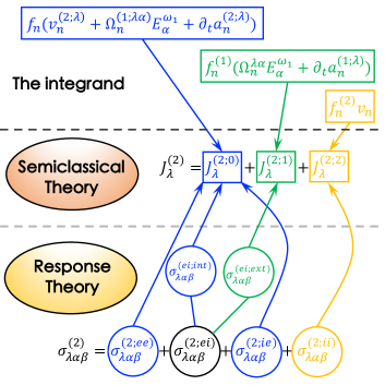
Figure 1: The schematic illustration about the equivalence between the AC semiclassical theory and the response theory. Here the middle panel displays the second-order current density given by the AC semiclassical theory, where the integrand for each term is placed into the top panel, and the bottom panel shows the second-order conductivity given by the response theory. The arrows with different colors are used to indicate the equivalence between both formulations.

IV Equivalence between the AC semiclassical theory and the response theory

Once the current density is obtained by the AC semiclassical theory and the response theory, we are ready to show that the current density given by both formulations are equivalent in the clean limit. To that purpose, we wish to remark that the the relaxation (indicated by $\tau$ or $\eta=1/\tau$ by way of solving the Boltzman equation) has been incorporated into the semiclassical expressions, while the conductivities given by the response theory does not include any relaxation effects. Therefore, the clean limit ($\eta\rightarrow 0$) will be adopted for the semiclassical expressions when needed.

In addition, we will also show that the relaxation can be introduced in the response theory by regularizing only the divergent terms. In doing so, two formalisms give the same result. In section V, we will discuss the consequence of other relaxation schemes such as Eq.(6) and show that it leads to a wrong result.

IV.1 The first order

At linear order, by comparing Eqs. (41-42) given by the AC semiclassical theory with Eqs. (51-52) given by the response theory, it is easy to find that

$$\sigma_{\lambda\alpha}^{(1;1)}E_{\alpha}^{\omega_{1}}=\lim_{\eta\rightarrow 0}J_{\lambda}^{(1;1)},\quad\sigma_{\lambda\alpha}^{(1;0)}E_{\alpha}^{\omega_{1}}=J_{\lambda}^{(1;0)},$$ (60)

which gives the well-known linear Drude current and anomalous Hall current, respectively. Particularly, in DC limit, we find

$$\lim_{\omega_{1}\rightarrow 0}\lim_{\eta\rightarrow 0}J_{\lambda}^{(1;1)} =\dfrac{1}{\xi}\sum_{n}\int_{k}\partial_{\alpha}f_{n}v_{n}^{\lambda}E_{\alpha}$$

$$=\lim_{\omega_{1}\rightarrow 0}\sigma^{(1;1)}_{\lambda\alpha}E_{\alpha}^{\omega_{1}},$$ (61)

In addition, we have

$$\lim_{\omega_{1}\rightarrow 0}\sigma_{\lambda\alpha}^{(1;0)}E_{\alpha}^{\omega_{1}}=\sum_{n}\int_{k}f_{n}\Omega_{n}^{\lambda\alpha}E_{\alpha}=\lim_{\omega_{1}\rightarrow 0}J_{\lambda}^{(1;0)}.$$ (62)

Furthermore, by inserting Eq.(26) into Eq.(43), we find

$$J_{\lambda}^{(1;0)} =\sum_{nm}\int_{k}f_{n}\left(\dfrac{r^{\lambda}_{nm}r^{\alpha}_{mn}\partial_{t}E_{\alpha}^{\omega_{1}}}{\omega_{1}-\epsilon_{mn}+i\xi}+\dfrac{r^{\lambda}_{mn}r^{\alpha}_{nm}\partial_{t}E_{\alpha}^{-\omega_{1}}}{\omega_{1}-\epsilon_{mn}-i\xi}\right)$$

$$=\sum_{nm}\int_{k}f_{nm}\dfrac{-i(\omega_{1}+i\xi)r^{\lambda}_{nm}r^{\alpha}_{mn}}{\omega_{1}-\epsilon_{mn}+i\xi}E_{\alpha}^{\omega_{1}}$$

$$=\sigma_{\lambda\alpha}^{(1;\bar{0})}E_{\alpha}^{\omega_{1}},$$ (63)

where we have used $\sum_{\omega_{1}=\pm\omega}h(\omega_{1})=\sum_{\omega_{1}=\pm\omega}h(-\omega_{1})$ for arbitrary function $h(\omega_{1})$ and interchanged $m$ and $n$ to obtain the second line. We wish to mention that Eq.(43) or the equivalent $\sigma_{\lambda\alpha}^{(1;\bar{0})}E_{\alpha}^{\omega_{1}}$ gives the displacement current under an AC electric field (vanishes in DC limit), which is intimately related to the quantum metric as recently discussed in Ref.[XiangDHE, ]. With Eqs. (60) and (63), we conclude that the AC semiclassical current at the linear order of electric field is equivalent to that given by response theory, even in DC limit.

In the presence of relaxation, by replacing $\xi$ by $1/\tau$ in divergent term Eq.(62) in the response theory we obtain the same expression as that of the semi-classical theory with $\eta=1/\tau$.

IV.2 The second order: the DC case

Since the AC semiclassical theory and the response theory give many terms at the second order of electric field, therefore, before considering the general situation we first show the equivalence between both formulations in DC limit, by carefully investigating the zero-frequency divergent behavior of both approaches in this limit. Note that in DC limit the contributions due to the time variation of positional shift in Eqs. (45) and (46) given by the semiclassical current do not appear.

In DC limit, by investigating the zero-frequency of both approaches, we note that Eq.(47) obtained with the AC semiclassical theory is equivalent to Eq.(58) obtained with the response theory. Explicitly, we find

$$\lim_{\omega_{i}\rightarrow 0}\lim_{\eta\rightarrow 0}J^{(2;2)}_{\lambda} =\dfrac{1}{\xi^{2}}\sum_{n}\int_{k}v_{n}^{\lambda}\partial^{2}_{\alpha\beta}E_{\alpha}E_{\beta}$$

$$=\lim_{\omega_{i}\rightarrow 0}\sigma^{(2;ii)}_{\lambda\alpha\beta}E_{\alpha}^{\omega_{1}}E_{\beta}^{\omega_{2}},$$ (64)

where the clean limit is taken for the semiclassical current $J^{(2;2)}_{\lambda}$ which diverges. In the presence of relaxation, $\xi^{2}=1/(2\tau^{2})$ BH-Yan is introduced on the same footing to regularize this divergent limit given by both approaches. As a result, Eq.(64) gives the familiar nonlinear Drude current which quadratically depends on the relaxation time $\tau$.

Following the same strategy, we next show that the AC semiclassical current $J^{(2;1)}_{\lambda}$ given by Eq.(46) in DC limit is encoded in the nonlinear conductivity $\sigma^{(2,ei)}_{\lambda\alpha\beta}$ given by Eq.(56) in the response theory. Particularly, by inserting Eq.(38) into Eq.(46), we first find that $J^{(2;1)}_{\lambda}$ in DC limit becomes

$$\lim_{\omega_{i}\rightarrow 0}\lim_{\eta\rightarrow 0}J^{(2;1)}_{\lambda} =\frac{1}{\xi}\sum_{n}\int_{k}\partial_{\beta}f_{n}\Omega_{n}^{\lambda\alpha}E_{\alpha}E_{\beta},$$ (65)

On the other hand, using $v^{\lambda}_{nm}=i\epsilon_{nm}r^{\lambda}_{nm}$ ($m\neq n$) and

$$\dfrac{\epsilon_{mn}}{(\omega_{\Sigma}-\epsilon_{mn}+2i\xi)(\omega_{1}+i\xi)}$$

$$=\dfrac{\epsilon_{mn}}{\omega_{2}-\epsilon_{mn}+i\xi}\left(\dfrac{1}{\omega_{1}+i\xi}-\dfrac{1}{\omega_{\Sigma}-\epsilon_{mn}+2i\xi}\right),$$ (66)

we find that Eq.(56) in DC limit can be decomposed as $\sigma^{(2;ei)}_{\lambda\alpha\beta}=\sigma^{(ei;ext)}_{\lambda\alpha\beta}+\sigma^{(ei;int)}_{\lambda\alpha\beta}$, where

$$\lim_{\omega_{i}\rightarrow 0}\sigma^{(ei;ext)}_{\lambda\alpha\beta} =\frac{1}{\xi}\sum_{mn}\int_{k}ir^{\lambda}_{nm}r^{\beta}_{mn}\partial_{\alpha}f_{nm},$$ (67)

$$\lim_{\omega_{i}\rightarrow 0}\sigma^{(ei;int)}_{\lambda\alpha\beta} =\sum_{mn}\int_{k}\dfrac{r^{\lambda}_{nm}r^{\beta}_{mn}\partial_{\alpha}f_{nm}}{-\epsilon_{mn}},$$ (68)

where the superscript $ext$ ($int$) stands for the extrinsic (intrinsic) contribution. By interchanging $m$ and $n$ of Eq.(67), it is easy to show that

$$\lim_{\omega_{i}\rightarrow 0}\sigma^{(ei;ext)}_{\lambda\alpha\beta}E_{\alpha}^{\omega_{1}}E_{\beta}^{\omega_{2}} =\frac{1}{\xi}\sum_{n}\int_{k}\partial_{\alpha}f_{n}\Omega^{\lambda\beta}_{n}E_{\alpha}E_{\beta}$$

$$=\lim_{\omega_{i}\rightarrow 0}\lim_{\eta\rightarrow 0}J^{(2;1)}_{\lambda},$$ (69)

which is nothing but the well-known extrinsic second-order nonlinear Hall current driven by the Berry curvature dipole BCD ; JEMoore2010 in the clean limit.

When the relaxation is present, it is a little bit tricky to regularize the divergence. It is clear from Eq.(66) that although it diverges but it also contains a non-divergence term (see the second term on the right hand side of Eq.(66)). The divergence of the left hand side of Eq.(66) is ”reducible” while the divergence of the first term on the right hand side of Eq.(66) is ”irreducible”. We only regularize the ”irreducible” part of divergence, i.e., we replace $\xi$ by $1/\tau$ only in Eq.(67) but leave the infinitesimal quantity $\xi$ in Eq.(68) unchanged. We will discuss this issue in more detail in section V.

Finally, we show that the intrinsic conductivity Eq.(68) together with the remaining conductivities (which can only contribute to the intrinsic current, as will be clear below) in response theory, namely, Eq.(55) and Eq.(57), is equivalent to the intrinsic current given by Eq.(45) in the AC semiclassical theory, particularly in DC limit. Explicitly, we will show:

$$\lim_{\omega_{i}\rightarrow 0}\lim_{\eta\rightarrow 0}J^{(2;0)}_{\lambda} =\lim_{\omega_{i}\rightarrow 0}\left[\sigma^{(2;ee)}_{\lambda\alpha\beta}+\sigma^{(2;ie)}_{\lambda\alpha\beta}+\sigma^{(ei;int)}_{\lambda\alpha\beta}\right]E_{\alpha}^{\omega_{1}}E_{\beta}^{\omega_{2}}.$$ (70)

To that purpose, by inserting Eq.(35) and $\Omega_{n}^{(1;\lambda\alpha)}=\partial_{\lambda}a_{n}^{(1;\alpha)}-\partial_{\alpha}a_{n}^{(1;\lambda)}$ into Eq.(45), we find that $J_{\lambda}^{(2;0)}$ given by the AC semiclassical theory in DC limit can be simplified as

$$\lim_{\omega_{i}\rightarrow 0}J_{\lambda}^{(2;0)}$$

$$=\sum_{n}\int_{k}f_{n}\left[-\dfrac{\partial_{\lambda}a_{n}^{(1;\beta)}}{2}+\left(\partial_{\lambda}a_{n}^{(1;\beta)}-\partial_{\beta}a_{n}^{(1;\lambda)}\right)\right]E_{\beta}$$

$$=\sum_{n}\int_{k}\left[a_{n}^{(1;\lambda)}-\dfrac{1}{2}a_{n}^{(1;\beta)}\partial_{\lambda}f_{n}\partial_{\beta}f_{n}\right]E_{\beta}$$

$$=\sum_{nm}\int_{k}\left(\dfrac{g^{\lambda\alpha}_{nm}}{\epsilon_{nm}}\partial_{\beta}f_{n}-\dfrac{g^{\beta\alpha}_{nm}}{2\epsilon_{nm}}\partial_{\lambda}f_{n}\right)E_{\alpha}E_{\beta}$$

$$=\dfrac{1}{2}\sum_{nm}\int_{k}\left(\dfrac{g^{\lambda\alpha}_{nm}}{\epsilon_{nm}}\partial_{\beta}f_{n}+\dfrac{g^{\lambda\beta}_{nm}}{\epsilon_{nm}}\partial_{\alpha}f_{n}-\dfrac{g^{\beta\alpha}_{nm}}{\epsilon_{nm}}\partial_{\lambda}f_{n}\right)E_{\alpha}E_{\beta},$$ (71)

where we have symmetrized the final result about the field indices. Note that in DC limit $a_{n}^{(1;\lambda)}=\sum_{m}g^{\lambda\alpha}_{nm}E_{\alpha}/\epsilon_{nm}$ with $g^{\lambda\alpha}_{nm}=r^{\lambda}_{nm}r^{\alpha}_{mn}+r^{\alpha}_{nm}r^{\lambda}_{mn}$ the quantum metric, which is symmetric about $\lambda$ and $\alpha$. On the other hand, by interchanging $m$ and $n$ and symmetrizing $\alpha$ and $\beta$, we find that Eq.(68) can be expressed as

$$\sigma^{(ei;int)}_{\lambda\alpha\beta} =\sum_{mn}\int_{k}\dfrac{1}{2}\left(\dfrac{g^{\lambda\beta}_{nm}}{\epsilon_{nm}}\partial_{\alpha}f_{n}+\dfrac{g^{\lambda\alpha}_{nm}}{\epsilon_{nm}}\partial_{\beta}f_{n}\right).$$ (72)

In addition, for $\sigma^{(2;ie)}_{\lambda\alpha\beta}$, in DC limit we find

$$\lim_{\omega_{i}\rightarrow 0}\sigma^{(2;ie)}_{\lambda\alpha\beta}=\sum_{mn}\int_{k}\dfrac{f_{nm}r^{\alpha}_{mn}}{\epsilon_{nm}}\mathcal{D}^{\beta}_{nm}r^{\lambda}_{nm}.$$ (73)

Furthermore, for $\sigma^{(2;ee)}_{\lambda\alpha\beta}$, when $m=n$ we find (see Appendix D.1 for details)

$$\sigma^{(2;ee)}_{\lambda\alpha\beta}(m=n)\equiv\sigma^{(2;ee1)}_{\lambda\alpha\beta}$$

$$=\dfrac{1}{2}\sum_{nm}\int_{k}\dfrac{\Delta^{\lambda}_{nm}f_{nm}r^{\beta}_{nm}r^{\alpha}_{mn}}{\left(\omega_{1}-\epsilon_{mn}+i\xi\right)\left(\omega_{2}+\epsilon_{mn}+i\xi\right)},$$ (74)

where $\Delta^{\lambda}_{nm}=v^{\lambda}_{n}-v^{\lambda}_{m}$. As shown in Appendix D.1, the divergent factor $1/(\omega_{\Sigma}+i2\xi)$ in $\sigma^{2;ee}_{\lambda\alpha\beta}(m=n)$ has been removed after symmetrization. In DC limit, we then obtain

$$\sigma_{\lambda\alpha\beta}^{(2;ee1)} \equiv\dfrac{1}{2}\sum_{nm}\int_{k}\dfrac{-\Delta^{\lambda}_{nm}f_{nm}r^{\beta}_{nm}r^{\alpha}_{mn}}{\epsilon_{nm}^{2}}$$

$$=\dfrac{1}{2}\sum_{nm}\int_{k}f_{n}g^{\beta\alpha}_{nm}\partial_{\lambda}\left(\dfrac{1}{\epsilon_{nm}}\right),$$ (75)

which is symmetric about the field indices $\alpha$ and $\beta$. When $m\neq n$, we can directly take the DC limit and obtain

$$\lim_{\omega_{i}\rightarrow 0}\sigma_{\lambda\alpha\beta}^{(2;ee)}(m\neq n)\equiv\lim_{\omega_{i}\rightarrow 0}\sigma_{\lambda\alpha\beta}^{(2;ee1)}$$ (76)

$$=\sum_{nml}\int_{k}ir^{\lambda}_{nm}\left(\dfrac{r^{\beta}_{ml}r^{\alpha}_{ln}f_{nl}}{-\epsilon_{ln}}-\dfrac{f_{lm}r^{\alpha}_{ml}r^{\beta}_{ln}}{-\epsilon_{ml}}\right)$$

$$=\sum_{nml}\int_{k}\dfrac{r^{\alpha}_{mn}f_{nm}}{\epsilon_{nm}}i\left(r^{\lambda}_{nl}r^{\beta}_{lm}-r^{\beta}_{nl}r^{\lambda}_{lm}\right)$$

$$=\sum_{nm}\int_{k}\dfrac{r^{\alpha}_{mn}f_{nm}}{\epsilon_{nm}}\left(\mathcal{D}^{\lambda}_{nm}r^{\beta}_{nm}-\mathcal{D}^{\beta}_{nm}r^{\lambda}_{nm}\right),$$ (77)

where we have used the relation Sipe2000

$$\mathcal{D}_{nm}^{\lambda}r^{\beta}_{nm}-\mathcal{D}_{nm}^{\beta}r^{\lambda}_{nm}=i\sum_{l}\left(r^{\lambda}_{nl}r^{\beta}_{lm}-r^{\beta}_{nl}r^{\lambda}_{lm}\right).$$ (78)

Combining Eq.(73), Eq.(75) and Eq.(77), we find

$$\lim_{\omega_{i}\rightarrow 0}\left(\sigma_{\lambda\alpha\beta}^{(2;ie)}+\sigma_{\lambda\alpha\beta}^{(2;ee)}\equiv\sigma_{\lambda\alpha\beta}^{(2;ie)}+\sigma_{\lambda\alpha\beta}^{(2;ee1)}+\sigma_{\lambda\alpha\beta}^{(2;ee2)}\right)$$

$$=\sum_{nm}\int_{k}\left[f_{nm}\dfrac{r^{\alpha}_{mn}f_{nm}}{\epsilon_{nm}}\mathcal{D}^{\lambda}_{nm}r^{\beta}_{nm}+\dfrac{1}{2}f_{n}g^{\beta\alpha}_{nm}\partial_{\lambda}\left(\dfrac{1}{\epsilon_{nm}}\right)\right]$$

$$=\dfrac{1}{2}\sum_{nm}\int_{k}f_{n}\left[\dfrac{1}{\epsilon_{nm}}\partial_{\lambda}g^{\beta\alpha}_{nm}+g^{\beta\alpha}_{nm}\partial_{\lambda}\left(\dfrac{1}{\epsilon_{nm}}\right)\right]$$

$$=-\dfrac{1}{2}\sum_{nm}\int_{k}\dfrac{g^{\beta\alpha}_{nm}}{\epsilon_{nm}}\partial_{\lambda}f_{n},$$ (79)

where we have symmetrized the first term of the second line about $\alpha$ and $\beta$ to obtain the final result and used Sipe2000

$$\partial_{\lambda}(r^{\alpha}_{nm}r^{\beta}_{mn})=\left(\mathcal{D}^{\lambda}_{nm}r^{\alpha}_{nm}\right)r^{\beta}_{mn}+r^{\alpha}_{nm}\left(\mathcal{D}^{\lambda}_{mn}r^{\beta}_{mn}\right).$$ (80)

By further combining Eq.(79) with Eq.(72), we finally arrive tat

$$\lim_{\omega_{i}\rightarrow 0}\left[\sigma_{\lambda\alpha\beta}^{(2;ie)}+\sigma_{\lambda\alpha\beta}^{(2;ee)}+\sigma_{\lambda\alpha\beta}^{(ei;int)}\right]E_{\alpha}^{\omega_{1}}E_{\beta}^{\omega_{2}}$$

$$=\dfrac{1}{2}\sum_{nm}\int_{k}\left(\dfrac{g^{\lambda\alpha}_{nm}}{\epsilon_{nm}}\partial_{\beta}f_{n}+\dfrac{g^{\lambda\beta}_{nm}}{\epsilon_{nm}}\partial_{\alpha}f_{n}-\dfrac{g^{\beta\alpha}_{nm}}{\epsilon_{nm}}\partial_{\lambda}f_{n}\right)E_{\alpha}E_{\beta}$$

$$=\lim_{\omega_{i}\rightarrow 0}J^{(2;0)}_{\lambda},$$ (81)

which shows that the second-order intrinsic current obtained with the response theory is also equivalent to that derived with the AC semiclassical theory, particularly in DC limit. Note that the second-order intrinsic current contains both the longitudinal (from the second-order energy correction $\epsilon_{n}^{(2)}$) and transverse (from the anomalous velocity $\bm{E}\times\bm{\Omega}_{n}^{(1)}$ and the second-order energy correction $\epsilon_{n}^{(2)}$) components, which can only appear in systems without $\mathcal{P}$ and $\mathcal{T}$ symmetries. At this stage, we wish to mention that the intrinsic second-order Ohmic current proposed in Refs. CulcerPRBL and GangSu2022 based on the response theory can also be reproduced by the semiclassical theory where the second-order energy must be taken into account (missed in Ref. CulcerPRBL ). As a result, the response theory does not contain any interband coherent correction compared to the semiclassical theory.

In the presence of relaxation, since there is no divergence in the intrinsic contribution, there is no need to introduce relaxation in this part and therefore two formalisms are also the same.

To clearly illustrate the equivalence between two formulations, we schematically summarized the main results obtained in this subsection into FIG.(1), which will be useful when we show that both formulations are equivalent in AC regime in the following, also in clean limit.

IV.3 The second order: the AC case

Guided by the equivalence between the semiclassical theory and the response theory in DC limit, as summarized in FIG.(1), we further show the equivalence between both approaches in the AC regime. First of all, it is easy to show that

$$\sigma_{\lambda\alpha\beta}^{(2;ii)}E_{\alpha}^{\omega_{1}}E_{\beta}^{\omega_{2}}=\lim_{\eta\rightarrow 0}J_{\lambda}^{(2;2)}$$ (82)

by using Eq.(58) and Eq.(47), in which Eq.(39) is inserted.

In DC case, we have shown that the conductivity $\sigma^{(2;ei)}_{\lambda\alpha\beta}$ is divided into the extrinsic and the intrinsic contributions. In AC case, we follow the same partition. In addition, we may expect some additional contribution that vanishes in DC limit, which should correspond to the displacement current given by the time variation of positional shift in the AC semiclassical theory. Particularly, using Eq.(66) and

$$\dfrac{\epsilon_{mn}}{\omega_{2}-\epsilon_{mn}+i\xi}=-1+\dfrac{\omega_{2}+i\xi}{\omega_{2}-\epsilon_{mn}+i\xi},$$ (83)

we can partition $\sigma_{\lambda\alpha\beta}^{(2;ei)}$ into $\sigma^{(2;ei)}_{\lambda\alpha\beta}\equiv\sigma^{(ei;1)}_{\lambda\alpha\beta}+\sigma^{(ei;0)}_{\lambda\alpha\beta}+\sigma^{(ei;\bar{1})}_{\lambda\alpha\beta}$, where

$$\sigma^{(ei;1)}_{\lambda\alpha\beta} =\sum_{mn}\int_{k}\dfrac{-r^{\lambda}_{nm}r^{\beta}_{mn}\partial_{\alpha}f_{nm}}{\omega_{1}+i\xi},$$ (84)

$$\sigma^{(ei;\bar{1})}_{\lambda\alpha\beta} =\sum_{mn}\int_{k}\dfrac{(\omega_{2}+i\xi)r^{\lambda}_{nm}r^{\beta}_{mn}\partial_{\alpha}f_{nm}}{(\omega_{2}-\epsilon_{mn}+i\xi)\left(\omega_{1}+i\xi\right)},$$ (85)

$$\sigma^{(ei;0)}_{\lambda\alpha\beta} \equiv\sum_{mn}\int_{k}\dfrac{-\epsilon_{mn}r^{\lambda}_{nm}r^{\beta}_{mn}\partial_{\alpha}f_{nm}}{(\omega_{2}-\epsilon_{mn}+i\xi)\left(\omega_{\Sigma}-\epsilon_{mn}+i2\xi\right)}$$

$$=\sum_{mn}\int_{k}\dfrac{-iv^{\lambda}_{nm}r^{\alpha}_{mn}\partial_{\beta}f_{nm}}{(\omega_{1}-\epsilon_{mn}+i\xi)\left(\omega_{\Sigma}-\epsilon_{mn}+i2\xi\right)}$$ (86)

where the superscripts $(ei;1)$, $(ei;\bar{1})$, and $(ei;0)$ stand for the extrinsic (existing in DC limit), AC (disappearing in AC limit), and intrinsic (existing in DC limit) contributions, respectively. As expected, we find

$$\left(\sigma_{\lambda\alpha\beta}^{(ei;1)}+\sigma_{\lambda\alpha\beta}^{(ei;\bar{1})}\right)E_{\alpha}^{\omega_{1}}E_{\beta}^{\omega_{2}}=\lim_{\eta\rightarrow 0}J_{\lambda}^{(2;1)},$$ (87)

where

$$\lim_{\eta\rightarrow 0}J_{\lambda}^{(2;1)}=\lim_{\eta\rightarrow 0}\sum_{n}\int_{k}f_{n}^{(1)}\left(\Omega^{\lambda\beta}_{n}E_{\beta}^{\omega_{2}}+\partial_{t}a_{n}^{(1;\lambda)}\right)$$

$$=\sum_{n}\int_{k}\dfrac{-r^{\lambda}_{nm}r^{\beta}_{mn}\partial_{\alpha}f_{nm}}{\omega_{1}+i\xi}E_{\alpha}^{\omega_{1}}E_{\beta}^{\omega_{2}}$$

$$+\sum_{mn}\int_{k}\dfrac{(\omega_{2}+i\xi)r^{\lambda}_{nm}r^{\beta}_{mn}\partial_{\alpha}f_{nm}}{(\omega_{2}-\epsilon_{mn}+i\xi)(\omega_{1}+i\xi)}E_{\alpha}^{\omega_{1}}E_{\beta}^{\omega_{2}}$$ (88)

by inserting Eq.(26) and Eq.(38) into Eq.(46). Note that $\Omega^{\lambda\beta}_{n}=\sum_{m}i(r^{\lambda}_{nm}r^{\beta}_{mn}-r^{\beta}_{nm}r^{\lambda}_{mn})$ and the second line is obtained by index interchanging.

For the remaining terms both in the response theory and in the AC semiclassical theory, we can also establish the following equivalent relation (see Appendix D.2 for details)

$$\left(\sigma_{\lambda\alpha\beta}^{(2;ee)}+\sigma_{\lambda\alpha\beta}^{(2;ie)}+\sigma_{\lambda\alpha\beta}^{(ei;0)}\right)E_{\alpha}^{\omega_{1}}E_{\beta}^{\omega_{2}}=J_{\lambda}^{(2;0)},$$ (89)

which is the same as the DC case, as illustrated in FIG.(1). In summary, the AC semiclassical theory is also equivalent to the response theory at the second order of the electric field, particularly in the clean limit.

Going beyond the clean limit, we introduce the relaxation in the AC response theory in exactly the same way as in DC response theory so that it not only leads to the correct DC limit and it also gives the same result as that of AC semi-classical theory as well.

V Consequences of the equivalence

In this section, we discuss the physical implications behind the equivalence between the AC semiclassical theory and the response theory. First of all, we wish to suggest that by expanding the energy of equilibrium Fermi distribution in terms of external field in the semiclassical theory to achieve nonlinear effects need more theoretical efforts since this correction does not appear in the clean limit. This is because for the semi-classical theory we usually refer two components: (1) semi-classical equation of motion Eqs.(1) and (2) solved by wavepacket method within Lagrange formalism; and (2) the Boltzmann equation Eq.(3) governing the Fermi distribution function for non-equilibrium situation. The use of $f({\tilde{\epsilon}}_{n})$ instead of $f({\epsilon}_{n})$ for equilibrium Fermi distribution function is actually not part of the conventional semi-classical theory. It is put in there by interpretation rather than derivation. Additionally, we illustrate that the distinctions between the AC semiclassical theory and the response theory is rooted in the way to introduce the relaxation. For the former, the relaxation is introduced by solving the Boltzmann equation. While for the latter, the relaxation is introduced by phenomenally modifying the quantum Liouville equation.

V.1 Energy used in the distribution function

Note that in the previous sections, we have assumed that the energy used in the equilibrium Fermi distribution function is the unperturbed band energy. Recently, some works obtained the third-order nonlinear Hall effect BPT ; TaIrTe4 ; Liu2022 ; Nandy by Taylor expanding the Fermi distribution function where the energy takes into account the correction due to external field. For instance, by replacing the unperturbed energy in $f_{n}^{(1)}$ with $\bar{\epsilon}_{n}=\epsilon_{n}+\epsilon_{n}^{(2)}$ and further Taylor expanding $f_{n}^{(1)}(\bar{\epsilon}_{n})$ as

$$f_{n}^{(1)}(\bar{\epsilon}_{n}) =\tau E_{\alpha}\partial_{\alpha}f_{n}(\bar{\epsilon}_{n})$$

$$=\tau E_{\alpha}\partial_{\alpha}f_{n}(\epsilon_{n})+\tau E_{\alpha}\partial_{\alpha}\left[\epsilon_{n}^{(2)}f_{n}^{\prime}(\epsilon_{n})\right],$$ (90)

where we have used Eq.(38) and taken the DC limit, one can immediately obtain an extrinsic third-order nonlinear current

$$J_{\lambda}=\tau\sum_{n}\int_{k}v_{n}^{\lambda}E_{\alpha}\partial_{\alpha}\left[\epsilon_{n}^{(2)}f_{n}^{\prime}(\epsilon_{n})\right].$$ (91)

by Taylor expanding $f_{n}^{(1)}(\bar{\epsilon}_{n})=f_{n}^{(1)}(\epsilon_{n})+f_{n}^{(1)^{\prime}}(\epsilon_{n})\epsilon_{n}^{(2)}+\cdots$, one can obtain a third-order nolinear current given by

$$\bm{J}^{(3)}=-\dfrac{1}{2}\sum_{n}\int_{k}f_{n}^{\prime\prime}\epsilon_{n}^{(2)}\bm{E}\times\bm{\Omega}_{n}\propto E_{\alpha}^{3},$$ (92)

However, based on the equivalence between both formulations, we conclude that this treatment is not allowed. Particularly, if we admit this expansion then we can immediately find an additional intrinsic second-order nonlinear current

$$J^{(2)}_{\lambda}=\sum_{n}\int_{k}f_{n}^{\prime}(\epsilon_{n})\epsilon_{n}^{(2)}v_{n}^{\lambda},$$ (93)

which clearly can not be reproduced by the response theory. As a result, the energy used in Fermi distribution in the semiclassical theory should be the unperturbed band energy like that in the response theory.

V.2 Phenomenological relaxation in the response theory

Next we discuss the phenomenological relaxation introduced in the response theory. We wish to mention that the conductivities Eqs.(55-58) particularly in the response theory are obtained by solving the standard quantum Liouville equation Eq.(4) and hence do not contain relaxation like the semiclassical theory, where the relaxation is explicitly introduced by solving the Boltzmann equation. Usually, to take explicitly the relaxation into account in the response theory, Eq.(4) is phenomenologically modified as Mikhailov ; Peres

$$i\partial_{t}\rho_{mn}=[H,\rho]_{mn}-\dfrac{i}{\tau}(\rho_{mn}-\rho^{(0)}_{mn}),$$ (94)

which has been used in many studies Sodemann2019 ; HWXu2021 ; Culcer2022 . Interestingly, we find that this phenomenological modification of Liouville equation leads to a unphysical result, where the linear intrinsic anomalous Hall current becomes a linear extrinsic current in DC limit which survives even for time-reversal invariant systems. Furthermore, it also breaks the equivalence between both formulations at both linear and nonlinear order of electric field.

To be specific, by comparing Eqs. (94) with (4) and then by replacing $i\epsilon_{mn}$ with $i\epsilon_{mn}+1/\tau$ in Eq.(52) (see Appendix C.3 for details), we find that the previous linear DC anomalous Hall conductivity becomes

$$\sigma_{\lambda\alpha}^{H} =2\sum_{mn}\int_{k}f_{n}\text{Re}\left[\dfrac{r^{\alpha}_{mn}v^{\lambda}_{nm}}{-\epsilon_{mn}+i/\tau}\right].$$ (95)

Let us examine Eq.(95) in more detail. For small relaxation limit (large $\tau$), we have the leading order $(1/\tau)\int_{k}f_{n}G_{\alpha\lambda}$ with $G_{\alpha\lambda}$ the Berry connection polarizability tensorGaoY2014 . For large relaxation limit (small $\tau$), we find that the linear extrinsic Hall conductivity is governed by quantum metric. In both limits, we find the linear extrinsic Hall conductivity which can be nonzero for time reversal invariant systems. This apparently contradicts with the understanding about the linear response of crystalline solids under the electric field. For the linear response driven by the DC electric field, we only have the extrinsic Drude current and the intrinsic anomalous Hall current for charge degree of freedom. For this reason, we will abandon Eq.(6).

Interestingly, if the phenomenological relaxation introduced in Eq.(94) is constrained to the intraband scattering, namely by modifying Eq.(94) into

$$i\partial_{t}\rho_{mn}=[H,\rho]_{mn}-\frac{i}{\tau}\delta_{mn}(\rho_{mn}-\rho^{(0)}_{mn}),$$ (96)

we find that the response theory (Note that $1/\tau$ disappears in Eq.(95) due to $m\neq n$) agrees perfectly with the semiclassical theory at the linear order of electric field. Unfortunately, Eq.(96) also leads to a unphysical result for the second order nonlinear conductivity in DC case as detailed below. In addition, both formulations are no longer equivalent at the second order of the electric field. Specifically, by comparing Eqs. (94) with (4) and then by replacing $i\epsilon_{mn}$ to $i\epsilon_{mn}+\delta_{mn}/\tau$ in Eqs.(55-58) (see Appendix C.3 for details), we find that Eqs. (55-58) become

$$\sigma_{\lambda\alpha\beta}^{(2,ee)} =\sum_{mnl}\int_{k}\dfrac{v^{\lambda}_{nm}}{\omega_{\Sigma}-\epsilon_{mn}+i(\bar{\eta}+2\xi)}\left(\dfrac{r^{\beta}_{ml}r^{\alpha}_{ln}f_{nl}}{\omega_{1}-\epsilon_{ln}+i\xi}-\dfrac{f_{lm}r^{\alpha}_{ml}r^{\beta}_{ln}}{\omega_{1}-\epsilon_{ml}+i\xi}\right),$$ (97)

$$\sigma_{\lambda\alpha\beta}^{(2,ei)} =\sum_{mn}\int_{k}\left(\dfrac{v^{\lambda}_{nm}}{\omega_{\Sigma}-\epsilon_{mn}+i2\xi}\right)\left(\dfrac{ir^{\beta}_{mn}\partial_{\alpha}f_{nm}}{\omega_{1}+i(\eta+\xi)}\right),$$ (98)

$$\sigma_{\lambda\alpha\beta}^{(2,ie)} =\sum_{mn}\int_{k}\left(\dfrac{v^{\lambda}_{nm}}{\omega_{\Sigma}-\epsilon_{mn}+2i\xi}\right)\mathcal{D}^{mn}_{\beta}\left(\dfrac{if_{nm}r^{\alpha}_{mn}}{\omega_{1}-\epsilon_{mn}+i\xi}\right),$$ (99)

$$\sigma_{\lambda\alpha\beta}^{(2,ii)} =\sum_{n}\int_{k}\dfrac{-v^{\lambda}_{n}\partial^{2}_{\alpha\beta}f_{n}}{\left[\omega_{1}+i(\eta+\xi)\right]\left[\omega_{\Sigma}+i(\eta+2\xi)\right]},$$ (100)

where $\bar{\eta}=\delta_{mn}\eta$ with $\eta=1/\tau$. At this point, we find that the extrinsic Drude and Hall currents given by the AC semiclassical theory in DC limit can be well reproduced by Eqs.(100) and (98) given by the modified response theory (Eq.(96)), respectively. However, we note that Eq.(97) given by the modified response theory in the clean limit ($\eta=0$) is not divergent when $m=n$ since the singularity at zero frequency is removable (see Eq.(154)). Thus this term should belong to an intrinsic contribution. When the relaxation is present, the zero frequency singularity in Eq.(97) can not be removed and it contributes to an extra term proportional to $i\eta/(\omega_{\Sigma}+i\eta)$ when $m=n$. In DC limit, this leads to an extra intrinsic contribution upon turning on the relaxation, which is unphysical. For large frequency regime with $\omega>>i/\tau$, we have a $\tau^{-1}$-dependent nonlinear extrinsic current. As a consequence, the intrinsic current given by the semiclassical theory in DC limit can no longer be reproduced by the modified response theory in terms of the correspondence illustrated in FIG.(1). Therefore Eq.(96) is also problematic due to the unphysical result.

As discussed in section IV, a scheme of introducing relaxation is proposed based on conventional regularizing diverging terms. Specifically, for a general AC expression obtained from the response theory, we first set frequency to zero and replace $\xi$ by $1/\tau$ in the ”irreducible” diverging terms. After that we restore the frequency in the expression. There is one exception which is the $\tau^{2}$ term in DC limit which one has to replace $\xi^{2}$ by $1/(2\tau^{2})$ BH-Yan . However, if one is willing to modify the relaxation part of Boltzmann equation (which is the last thing we want to do), the substitution of $\xi$ by $1/\tau$ will be fine for the $\tau^{2}$ term in DC limit as well. Specifically, in DC limit, the modified solution of the non-equilibrium Fermi distribution ${\bar{f}}_{n}$ is of the form

$${\bar{f}}_{n}=f(\epsilon_{n}({\bf k}+\tau{\bf E}))\equiv f_{n}({\bf k}+\tau{\bf E})=\sum_{m}\frac{\tau^{m}}{m!}({\bf E}\cdot\nabla_{k})^{m}f_{n}$$ (101)

whereas the solution of the conventional Boltzmann equation is of the form

$${\bar{f}}_{n}=\sum_{m}\tau^{m}({\bf E}\cdot\nabla_{k})^{m}f_{n}.$$ (102)

The physical picture of solution Eq.(101) is that under the relaxation the non-equilibrium Fermi distribution has the same form as the equilibrium distribution with its momentum shifted by a constant amount $\tau{\bf E}$.

At this stage, we can not rule out other ways of introducing the relaxation as long as it will not lead to unphysical results. To close this section, we conclude that the distinction between the AC semiclassical theory and the response theory is rooted in the different ways of introducing the relaxation.

VI Discussion and Summary

First of all, although we stop at the second order of electric field, we believe that the equivalence between both formulations can be extended to higher-order, such as the third-order. Second, we wish to mention that the response theory used in this work is formulated at length gauge. Recently, some second-order nonlinear currents BH-Yan ; Kapla2023 based on response theory particularly at velocity gauge are proposed, which can also not be reproduced by the AC semiclassical theory and are treated as the quantum correction beyond the semiclassical theory. However, based on the equivalence between both formulations, we believe that these quantum correction may also be rooted in different ways of introducing phenomenological relaxation. In addition, we wish to remark that the $\tau^{-1}$-dependent nonlinear current obtained with response theory at length gauge may also be related to the different scheme of phenomenological relaxation Watanabe ; footnote2 . Finally, we did not discuss the consequences of the side jump and skew scattering Nagaosa2010 ; JTsong2023 ; CulcerPRBL ; XiaoCdisorder which is beyond the scope of this work.

In summary, by extending the conventional semiclassical theory under a uniform electric field to the AC nonlinear regime, we show that up to the second order of electric field, the AC semiclassical theory is equivalent to the response theory in clean limit and this equivalence can be expected even in DC limit when the zero-frequency divergence is properly regulated by introducing the relaxation on the same footing. In particular, at the linear order of the electric field, we show that both formulations can give the linear Drude current, intrinsic anomalous Hall current, and the displacement current, in which the last one arising from the time variation of the first-order positional shift can only be driven by a AC field and is usually overlooked even in AC transport. Furthermore, at the second order of the electric field, we show that all the well-known transport effects, including the nonlinear Drude current, the nonlinear Hall current that driven by the Berry curvature dipole and quantum metric dipole, respectively, can be obtained by both formulations. In addition, we find that the nonlinear displacement current due to the second-order position shift and the nonlinear intrinsic current due to the band energy correction in AC semiclassical theory can also be reproduced by the response theory. Finally, based on the equivalence, we suggest that the energy used in the equilibrium Fermi distribution may not contains the correction due to the electric field even when the rexlation is present and we conclude that the distinctions between both formulation are rooted in the different schemes of relaxation, which may lead to these additional quantum corrected nonlinear currents beyond the semiclassical theory.

VII Appendix

Appendix A Calculation details in Section II

A.1 Eqs.(25-27)

With the normalized second-order wavepacket Eq.(24), the position center $\bm{r}_{c}$ can be expressed as

$$\bm{r}_{c}\equiv\langle\bar{W}|\bm{r}|\bar{W}\rangle=(1+2\delta)\langle W_{0}|\bm{r}|W_{0}\rangle+2\text{Re}\langle W_{0}|\bm{r}|W_{1}\rangle+\langle W_{1}|\bm{r}|W_{1}\rangle+2\text{Re}\langle W_{0}|\bm{r}|W_{2}\rangle+\mathcal{O}(E_{\alpha}^{3}).$$ (103)

For $\langle W_{0}|\bm{r}|W_{0}\rangle$, we find Xiao2010

$$\langle W_{0}|\bm{r}|W_{0}\rangle =\int_{\bm{p}}\int_{\bm{p}^{\prime}}C_{n}(\bm{p})C_{n}^{*}(\bm{p}^{\prime})e^{i(\bm{p}-\bm{p}^{\prime})\cdot\bm{r}}\langle u_{n}^{\prime}|\bm{r}|u_{n}\rangle=\int_{\bm{p}}\int_{\bm{p}^{\prime}}C_{n}(\bm{p})C_{n}^{*}(\bm{p}^{\prime})\left[-i\partial_{\bm{p}}+\bm{\mathcal{A}}_{n}\right]\delta(\bm{p}-\bm{p}^{\prime})\partial_{\bm{p}_{c}}\gamma(\bm{p}_{c})+\bm{\mathcal{A}}_{n}(\bm{p}_{c}).$$ (104)

where we have used $|C_{n}(\bm{p})|^{2}=\delta(\bm{p}-\bm{p}_{c})$. In addition, we have assumed that $C_{n}(\bm{p})=|C_{n}(\bm{p})|e^{-i\gamma(\bm{p})}$ and used that

$$\int_{\bm{p}}\int_{\bm{p}^{\prime}}C_{n}(\bm{p})C_{n}^{*}(\bm{p}^{\prime})(-i\partial_{\bm{p}})\delta(\bm{p}-\bm{p}^{\prime}) =\int_{\bm{p}}\left[i\partial_{\bm{p}}C_{n}(\bm{p})\right]C_{n}^{*}(\bm{p})=\int_{\bm{p}}\partial_{\bm{p}}\gamma(\bm{p})|C_{n}(\bm{p})|^{2}+\int_{\bm{p}}|C_{n}(\bm{p})|i\partial_{\bm{p}}|C_{n}(\bm{p})|$$

$$=\partial_{\bm{p}_{c}}\gamma(\bm{p}_{c})+\dfrac{i}{2}\partial_{\bm{p}}\left(\int_{\bm{p}}|C_{n}(\bm{p})|^{2}\right)=\partial_{\bm{p}_{c}}\gamma(\bm{p}_{c}).$$ (105)

For $2\text{Re}\langle W_{0}|\bm{r}|W_{1}\rangle$, we find

$$2\text{Re}\langle W_{0}|\bm{r}|W_{1}\rangle=2\text{Re}\left[\int_{\bm{p}}\int_{\bm{p}^{\prime}}\sum_{m\neq n}M_{mn}^{(1)}(\bm{p})C_{n}(\bm{p})C_{n}^{*}(\bm{p}^{\prime})e^{i(\bm{p}-\bm{p}^{\prime})\cdot\bm{r}}\langle u_{n}^{\prime}|\bm{r}|u_{m}\rangle\right]=2\text{Re}\sum_{m}M_{mn}^{(1)}(\bm{p}_{c})\bm{r}_{nm}(\bm{p}_{c}).$$ (106)

Similarly, for $2\text{Re}\langle W_{0}|\bm{r}|W_{2}\rangle$, we find

$$2\text{Re}\langle W_{0}|\bm{r}|W_{2}\rangle=2\text{Re}\left[\int_{\bm{p}}\int_{\bm{p}^{\prime}}\sum_{m\neq n}M_{mn}^{(2)}(\bm{p})C_{n}(\bm{p})C_{n}^{*}(\bm{p}^{\prime})e^{i(\bm{p}-\bm{p}^{\prime})\cdot\bm{r}}\langle u_{n}^{\prime}|\bm{r}|u_{m}\rangle\right]=2\text{Re}\sum_{m}M_{mn}^{(2)}(\bm{p}_{c})\bm{r}_{nm}(\bm{p}_{c}).$$ (107)

Finally, for $\langle W_{1}|\bm{r}|W_{1}\rangle$, we find:

$$\langle W_{1}|\bm{r}|W_{1}\rangle=\int_{\bm{p}}\int_{\bm{p}^{\prime}}\sum_{m\neq n}\sum_{l\neq n}M_{mn}^{(1)}(\bm{p})M_{ln}^{(1)*}(\bm{p}^{\prime})C_{n}(\bm{p})C_{n}^{*}(\bm{p}^{\prime})e^{i(\bm{p}-\bm{p}^{\prime})\cdot\bm{r}}\langle u_{l}^{\prime}|\bm{r}|u_{m}\rangle$$

$$=\int_{\bm{p}}\int_{\bm{p}^{\prime}}\sum_{m\neq n}\sum_{l\neq n}M_{mn}^{(1)}(\bm{p})M_{ln}^{(1)*}(\bm{p}^{\prime})C_{n}(\bm{p})C_{n}^{*}(\bm{p}^{\prime})[-i\delta_{ln}\partial_{\bm{p}}+\bm{\mathcal{A}}_{lm}]\delta(\bm{p}^{\prime}-\bm{p})$$

$$=\int_{\bm{p}}\sum_{m\neq n}M_{mn}^{(1)*}(\bm{p})C_{n}^{*}(\bm{p})i\partial_{\bm{p}}\left[M_{mn}^{(1)}(\bm{p})C_{n}(\bm{p})\right]+\sum_{l\neq n}\sum_{m\neq n}M_{ln}^{(1)*}(\bm{p}_{c})\bm{\mathcal{A}}_{lm}(\bm{p}_{c})M_{mn}^{(1)}(\bm{p}_{c})$$

$$=\sum_{m\neq n}M_{mn}^{(1)*}(\bm{p}_{c})i\partial_{\bm{p}_{c}}M_{mn}^{(1)}(\bm{p}_{c})+\partial_{\bm{p}_{c}}\gamma(\bm{p}_{c})\sum_{m\neq n}M_{mn}^{(1)*}(\bm{p}_{c})M_{mn}^{(1)}(\bm{p}_{c})+\sum_{l\neq n}\sum_{m\neq n}M_{ln}^{(1)*}(\bm{p}_{c})\bm{\mathcal{A}}_{lm}(\bm{p}_{c})M_{mn}^{(1)}(\bm{p}_{c})$$

$$+\sum_{m\neq n}\int_{\bm{p}}M_{mn}^{(1)*}(\bm{p})M_{mn}^{(1)}(\bm{p})\dfrac{i}{2}\partial_{\bm{p}}|C_{n}(\bm{p})|^{2}$$

$$=\sum_{m\neq n}M_{mn}^{(1)*}(\bm{p}_{c})i\partial_{\bm{p}_{c}}M_{mn}^{(1)}(\bm{p}_{c})+\partial_{\bm{p}_{c}}\gamma(\bm{p}_{c})\sum_{m\neq n}M_{mn}^{(1)*}(\bm{p}_{c})M_{mn}^{(1)}(\bm{p}_{c})+\sum_{l\neq n}\sum_{m\neq n}M_{ln}^{(1)*}(\bm{p}_{c})\bm{\mathcal{A}}_{lm}(\bm{p}_{c})M_{mn}^{(1)}(\bm{p}_{c})$$

$$-\sum_{m\neq n}\dfrac{1}{2}i\partial_{\bm{p}_{c}}\left[M_{mn}^{(1)*}(\bm{p}_{c})M_{mn}^{(1)}(\bm{p}_{c})\right]$$

$$=\text{Re}\sum_{m\neq n}M_{mn}^{(1)*}(\bm{p}_{c})i\partial_{\bm{p}_{c}}M_{mn}^{(1)}(\bm{p}_{c})+\partial_{\bm{p}_{c}}\gamma(\bm{p}_{c})\sum_{m\neq n}M_{mn}^{(1)*}(\bm{p}_{c})M_{mn}^{(1)}(\bm{p}_{c})+\sum_{l\neq n}\sum_{m\neq n}M_{ln}^{(1)*}(\bm{p}_{c})\bm{\mathcal{A}}_{lm}(\bm{p}_{c})M_{mn}^{(1)}(\bm{p}_{c}).$$ (108)

Collecting these results, we obtain (for simplicity, we will drop the explicit dependence on $\bm{p}_{c}$ below)

$$\bm{r}_{c}=\partial_{\bm{p}_{c}}\gamma+\bm{\mathcal{A}}_{n}+\bm{a}_{n}^{(1)}+\bm{a}_{n}^{(2)},$$ (109)

as given by Eq.(25) in the main text. Here $\bm{a}_{n}^{(i)}$ is the $i$th positional shift given by

$$\bm{a}_{n}^{(1)}\equiv 2\text{Re}\langle W_{0}|\bm{r}|W_{1}\rangle=2\text{Re}\sum_{m}M_{mn}^{(1)}\bm{r}_{nm}$$ (110)

and

$$\bm{a}_{n}^{(2)}\equiv 2\delta\langle W_{0}|\bm{r}|W_{0}\rangle+2\text{Re}\langle W_{0}|\bm{r}|W_{2}\rangle+\langle W_{1}|\bm{r}|W_{1}\rangle$$

$$=-\sum_{m\neq n}M_{mn}^{(1)}\bm{\mathcal{A}}_{n}M_{mn}^{(1)*}+2\text{Re}\sum_{m\neq n}M_{mn}^{(2)}\bm{r}_{nm}+\text{Re}\sum_{m\neq n}M_{mn}^{(1)*}i\partial_{\bm{p}_{c}}M_{mn}^{(1)}+\sum_{l\neq n}\sum_{m\neq n}M_{ln}^{(1)*}\bm{\mathcal{A}}_{lm}M_{mn}^{(1)}$$

$$=\text{Re}\sum_{m}M_{mn}^{(1)*}i\bm{\mathcal{D}}^{\bm{p}_{c}}_{mn}M_{mn}^{(1)}+\sum_{ml}M_{ln}^{(1)*}\bm{r}_{lm}M_{mn}^{(1)}+2\text{Re}\sum_{m}M_{mn}^{(2)}\bm{r}_{nm}$$

$$=-\text{Re}\sum_{m}M_{mn}^{(1)}i\bm{\mathcal{D}}^{\bm{p}_{c}}_{nm}M_{mn}^{(1)*}+\sum_{ml}M_{ln}^{(1)*}\bm{r}_{lm}M_{mn}^{(1)}+2\text{Re}\sum_{m}M_{mn}^{(2)}\bm{r}_{nm}$$ (111)

where $2\delta\partial_{\bm{p}_{c}}\gamma$ is exactly canceled out with the second term of Eq.(108). Furthermore, using the Levi-Civita symbol and Eq.(18), we finally find:

$$a_{n}^{(1;\lambda)} =2\text{Re}\sum_{m}\sum_{\omega_{1}}\dfrac{r^{\lambda}_{nm}r^{\alpha}_{mn}}{\omega_{1}-\epsilon_{mn}+i\xi}E_{\alpha}^{\omega_{1}},$$ (112)

where $E_{\alpha}^{\omega_{1}}\equiv e^{-i(\omega_{1}+i\xi)t}$, as given by Eq.(26) in the main text. Furthermore, by using Eq.(18) and Eq.(20), we find

$$a_{n}^{(2;\lambda)} =\text{Re}\sum_{\omega_{1}\omega_{2}}\sum_{ml}\dfrac{2r^{\lambda}_{nm}r^{\beta}_{ml}r^{\alpha}_{ln}}{(\omega_{1}-\epsilon_{ln}+i\xi)(\omega_{\Sigma}-\epsilon_{mn}+2i\xi)}E_{\alpha}^{\omega_{1}}E_{\beta}^{\omega_{2}}$$

$$+\sum_{\omega_{1}\omega_{2}}\sum_{ml}\dfrac{-r^{\beta}_{nl}r^{\lambda}_{lm}r^{\alpha}_{mn}}{(\omega_{2}-\epsilon_{nl}+i\xi)(\omega_{1}-\epsilon_{mn}+i\xi)}E_{\alpha}^{\omega_{1}}E_{\beta}^{\omega_{2}}$$

$$+\text{Re}\sum_{\omega_{1}\omega_{2}}\sum_{m}\dfrac{2r^{\lambda}_{nm}}{\omega_{\Sigma}-\epsilon_{mn}+2i\xi}i\mathcal{D}^{\beta}_{mn}\left(\dfrac{r^{\alpha}_{mn}}{\omega_{1}-\epsilon_{mn}+i\xi}\right)E_{\alpha}^{\omega_{1}}E_{\beta}^{\omega_{2}}$$

$$+\text{Re}\sum_{\omega_{1}\omega_{2}}\sum_{m}\dfrac{r^{\beta}_{mn}}{\omega_{2}-\epsilon_{mn}+i\xi}i\mathcal{D}^{\lambda}_{nm}\left(\dfrac{r^{\alpha}_{nm}}{\omega_{1}-\epsilon_{nm}+i\xi}\right)E_{\alpha}^{\omega_{1}}E_{\beta}^{\omega_{2}}$$ (113)

as given by Eq.(27) in the main text, where we have used that

$$M_{mn}^{(1)*}=\sum_{\omega_{1}}\dfrac{r^{\alpha}_{nm}E_{\alpha}e^{i(\omega_{1}-i\xi)t}}{\omega_{1}-\epsilon_{mn}-i\xi}=\sum_{\omega_{1}}\dfrac{r^{\alpha}_{nm}E_{\alpha}e^{-i(\omega_{1}+i\xi)t}}{-\omega_{1}-\epsilon_{mn}-i\xi}=-M_{nm}^{(1)}$$ (114)

due to $\sum_{\omega_{1}=\pm\omega}f(\omega_{1})=\sum_{\omega_{1}=\pm\omega}f(-\omega_{1})$ for an arbitrary function $f(\omega_{1})$.

A.2 Eqs.(34-35)

With the second-order wavepacket Eq.(24), the energy for the wavepacket can be expressed as

$$\bar{\epsilon}_{n} \equiv\langle W_{0}|i\partial_{t}|W_{0}\rangle-\langle\bar{W}|(i\partial_{t}-H)|\bar{W}\rangle$$

$$=\left[-\langle W_{0}|i\partial_{t}\left(\delta|W_{0}\rangle\right)-\delta\langle W_{0}|i\partial_{t}|W_{0}\rangle-\langle W_{1}|i\partial_{t}|W_{1}\rangle\right]$$

$$+\left[\left(1+2\delta\right)\langle W_{0}|H_{0}|W_{0}\rangle+\langle W_{1}|H_{0}|W_{1}\rangle+\bm{E}\cdot\langle\bar{W}|\bm{r}|\bar{W}\rangle\right]+\mathcal{O}(E^{3})$$

$$=\left[-i\partial_{t}\delta-2\delta\partial_{t}\gamma-\langle W_{1}|i\partial_{t}|W_{1}\rangle\right]+\left[(1+2\delta)\epsilon_{n}+\sum_{m}M_{mn}^{(1)}M_{mn}^{(1)*}\epsilon_{m}+\bm{E}\cdot\bm{r}_{c}\right]+\mathcal{O}(E^{3}),$$ (115)

where we have used Eq.(29), $\langle W_{0}|W_{1}\rangle=0$, and $\langle W_{0}|W_{2}\rangle=0$. Note that

$$\langle W_{1}|i\partial_{t}|W_{1}\rangle=\int_{\bm{p}}\int_{\bm{p}^{\prime}}\sum_{m\neq n}\sum_{l\neq n}e^{i(\bm{p}-\bm{p}^{\prime})\cdot\bm{r}}M_{ln}^{(1)*}(\bm{p}^{\prime})\langle u_{l}^{\prime}|C_{n}(\bm{p}^{\prime})i\partial_{t}\left(M_{mn}^{(1)}(\bm{p})C_{n}(\bm{p})|u_{m}\rangle\right)$$

$$=\sum_{m}M_{mn}^{(1)}i\partial_{t}M_{mn}^{(1)*}+\int_{\bm{p}}\sum_{m}M_{mn}^{(1)*}(\bm{p})M_{mn}^{(1)}(\bm{p})C_{n}(\bm{p})i\partial_{t}C_{n}(\bm{p})$$

$$=\sum_{m}M_{mn}^{(1)}i\partial_{t}M_{mn}^{(1)*}+\partial_{t}\gamma\sum_{m}M_{mn}^{(1)}M_{mn}^{(1)*}+\int_{\bm{p}}\sum_{m}M_{mn}^{(1)*}(\bm{p})M_{mn}^{(1)}(\bm{p})\dfrac{i}{2}\partial_{t}|C_{n}(\bm{p})|^{2}$$

$$=\sum_{m}M_{mn}^{(1)}i\partial_{t}M_{mn}^{(1)*}+\partial_{t}\gamma\sum_{m}M_{mn}^{(1)}M_{mn}^{(1)*}+\sum_{m}\dfrac{i}{2}\partial_{t}\left(\int_{\bm{p}}M_{mn}^{(1)*}(\bm{p})M_{mn}^{(1)}(\bm{p})|C_{n}(\bm{p})|^{2}\right)$$

$$-\sum_{m}\int_{\bm{p}}\dfrac{i}{2}\partial_{t}\left(M_{mn}^{(1)*}(\bm{p})M_{mn}^{(1)}(\bm{p})\right)|C_{n}(\bm{p})|^{2}$$

$$=\sum_{m}M_{mn}^{(1)}i\partial_{t}M_{mn}^{(1)*}-2\delta\partial_{t}\gamma,$$ (116)

where we have used Eq.(23). Substituting Eq.(116) into Eq.(117), we find:

$$\bar{\epsilon}_{n} =\epsilon_{n}+\bm{E}\cdot\bm{r}_{c}+\dfrac{1}{2}i\partial_{t}\left(\sum_{m}M_{mn}^{(1)}M_{mn}^{(1)*}\right)-\sum_{m}M_{mn}^{(1)}i\partial_{t}M_{mn}^{(1)*}+\sum_{m}\epsilon_{mn}M_{mn}^{(1)}M_{mn}^{(1)*}+\mathcal{O}(E^{3})$$

$$=\epsilon_{n}+\bm{E}\cdot\bm{r}_{c}+\dfrac{1}{2}\sum_{m}\left[\left(i\partial_{t}M_{mn}^{(1)}\right)M_{mn}^{(1)*}-M_{mn}^{(1)}i\partial_{t}M_{mn}^{(1)*}\right]+\sum_{m}\epsilon_{mn}M_{mn}^{(1)}M_{mn}^{(1)*}+\mathcal{O}(E^{3})$$

$$=\epsilon_{n}+\bm{E}\cdot\bm{r}_{c}+\text{Re}\sum_{m}\left[\left(i\partial_{t}M_{mn}^{(1)}\right)M_{mn}^{(1)*}+\epsilon_{mn}M_{mn}^{(1)}M_{mn}^{(1)*}\right]$$

$$=\epsilon_{n}+\bm{E}\cdot\bm{r}_{c}+\epsilon^{(2)}_{n}+\mathcal{O}(E^{3}),$$ (117)

as given by Eq.(34) in the main text, where $\bm{r}_{c}\equiv\langle\bar{W}|\bm{r}|\bar{W}\rangle$ and

$$\epsilon_{n}^{(2)} \equiv\text{Re}\sum_{m}\left[\left(i\partial_{t}M_{mn}^{(1)}\right)M_{mn}^{(1)*}+\epsilon_{mn}M_{mn}^{(1)}M_{mn}^{(1)*}\right]=-\text{Re}\sum_{m}\sum_{\omega_{1}\omega_{2}}\dfrac{(\omega_{1}+i\xi+\epsilon_{mn})r_{mn}^{\alpha}r^{\beta}_{nm}E_{\alpha}^{\omega_{1}}E_{\beta}^{\omega_{2}}}{(\omega_{1}-\epsilon_{mn}+i\xi)(\omega_{2}-\epsilon_{nm}+i\xi)}$$

$$=-\text{Re}\sum_{m}\sum_{\omega_{1}\omega_{2}}\dfrac{r_{mn}^{\alpha}r^{\beta}_{nm}E_{\alpha}^{\omega_{1}}E_{\beta}^{\omega_{2}}}{\omega_{2}-\epsilon_{nm}+i\xi}=-\dfrac{1}{2}\sum_{\omega_{1}}a_{n}^{(1;\alpha)}E_{\alpha}^{\omega_{1}},$$ (118)

as given by Eq.(35) in the main text, where we have used $M_{mn}^{(1)*}=-M_{nm}^{(1)}$ and Eq.(26). Note that only the first term of Eq.(117) contains $\bm{r}_{c}$ while Eq.(118) depends only on $\bm{k}_{c}$.

Appendix B The solution for Boltzmann equation

In this appendix, we will derive Eq.(38) and Eq.(39) given in the main text, which are obtained by solving the Boltzmann equation in presence of the electric field. For completeness, the Boltzmann equation is reproduced as follows:

$$\partial_{t}\bar{f}_{n}+\eta(\bar{f}_{n}-f_{n}^{(0)})=E_{\alpha}^{\omega_{1}}\partial_{\alpha}\bar{f}_{n},$$ (119)

where the relaxation time approximation $\tau=1/\eta$ is adopted. Eq.(119) can be iteratively solved from the equilibrium distribution function $f_{n}^{(0)}=f_{n}=1/\left[e^{(\epsilon_{n}-\mu)/k_{B}T}+1\right]$ without the electric field, where $\mu$ is the chemical potential, $k_{B}$ is the Boltzmann constant, and $T$ is the temperature. Straightfowardly, by inserting $\bar{f}_{n}=f_{n}^{(0)}+f_{n}^{(1)}+f_{n}^{(2)}+\cdots$ into Eq.(119), where $f_{n}^{(i)}\propto E_{\alpha}^{(i)}$, we obtain the following recursive first-order inhomogeneous linear differential equation equations for the nonequilibrium distribution:

$$\partial_{t}f_{n}^{(1)}+\eta f_{n}^{(1)} =E_{\alpha}^{\omega_{1}}\partial_{\alpha}f_{n}^{(0)},$$ (120)

$$\partial_{t}f_{n}^{(2)}+\eta f_{n}^{(2)} =E_{\beta}^{\omega_{2}}\partial_{\beta}f_{n}^{(1)},$$ (121)

which are truncated at the second order of the electric field. Note that $f_{n}^{(i)}=0$ with $i=1,2$ in the absence of the electric field $(t\rightarrow-\infty)$ is the boundary condition for Eqs.(120-121). Recall that for the first-order inhomogeneous linear differential equation $\partial_{t}y(t)+p(t)y(t)=q(t)$, the general solution is given by

$$y(t)=e^{-\int p(t)dt}\left(C+\int q(t)e^{\int p(t)dt}dt\right).$$ (122)

Using Eq.(122), for Eq.(120), we immediately obtain

$$f_{n}^{(1)}=e^{-\eta t}\left(C+E_{\alpha}\partial_{\alpha}f_{n}^{(0)}\int e^{-i\left[\omega_{1}+i(\eta+\xi)\right]t}dt\right)=\dfrac{E_{\alpha}^{\omega_{1}}\partial_{\alpha}f_{n}^{(0)}}{-i\left[\omega_{1}+i(\eta+\xi)\right]}=\dfrac{i\partial_{\alpha}f_{n}^{(0)}E_{\alpha}^{\omega_{1}}}{\omega_{1}+i(\eta+\xi)},$$ (123)

where $p(t)=\eta$ and $q(t)=E_{\alpha}^{\omega_{1}}\partial_{\alpha}f_{n}^{(0)}$ in Eq.(122) and $C=0$ fixed by the boundary condition. Similarly, for Eq.(121), we obtain

$$f_{n}^{(2)} =e^{-\eta t}\left(C+\dfrac{i\partial_{\beta\alpha}^{2}f_{n}^{(0)}}{\omega_{1}+i(\eta+\xi)}\int e^{-i\left[\omega_{\Sigma}+i(\eta+2\xi)\right]t}dt\right)=\dfrac{E_{\alpha}^{\omega_{1}}E_{\beta}^{\omega_{2}}i\partial_{\alpha\beta}^{2}f_{n}^{(0)}}{\left[\omega_{1}+i(\eta+\xi)\right]\left[-i\omega_{\Sigma}+(\eta+2\xi)\right]}$$

$$=\dfrac{-\partial_{\alpha\beta}^{2}f_{n}^{(0)}E_{\alpha}^{\omega_{1}}E_{\beta}^{\omega_{2}}}{\left[\omega+i(\eta+\xi)\right]\left[\omega_{\Sigma}+i(\eta+2\xi)\right]},$$ (124)

where $q(t)=f_{n}^{(1)}$ has been used in Eq.(122). Eq.(123) and Eq.(39) are given by Eq.(38) and Eq.(39) in the main text, respectively.

Appendix C Response theory

In this appendix, we first derive the expressions for the density matrix element by iteratively solving the quantum Liouville equation. With the density matrix element, we further derive the linear and nonlinear conductivities given in the main text.

C.1 The density matrix element

The quantum Liouville equation for the density matrix in Bloch basis is reproduced as

$$i\partial_{t}\rho_{mn}=[H,\rho]_{mn}=\epsilon_{mn}\rho_{mn}+[r^{\alpha},\rho]_{mn}E_{\alpha}^{\omega_{1}},$$ (125)

where $\epsilon_{mn}=\epsilon_{m}-\epsilon_{n}$ and

$$[r^{\alpha},\rho]_{mn}=i\mathcal{D}^{\alpha}_{mn}\rho_{mn}+\sum_{l}\left(r^{\alpha}_{ml}\rho_{ln}-\rho_{ml}r^{\alpha}_{ln}\right).$$ (126)

Here $\mathcal{D}^{\alpha}_{mn}\equiv\partial_{\alpha}-i(\mathcal{A}_{m}^{\alpha}-\mathcal{A}_{n}^{\alpha})$ is the $U(1)$ covariant derivative. Eq.(125) can also be solved iteratively. Particularly, by writing $\rho_{mn}=\sum_{i}\rho_{mn}^{(i)}$, where $\rho_{mn}^{(i)}\propto E_{\alpha}^{(i)}$ and $\rho^{(0)}_{mn}=\delta_{mn}f_{n}$, we obtain the following recursive first-order inhomogeneous linear differential equations up to the second order of the electric field:

$$\partial_{t}\rho_{mn}^{(1)}+i\epsilon_{mn}\rho_{mn}^{(1)} =-i[r^{\alpha},\rho^{(0)}]_{mn}E_{\alpha}^{\omega_{1}}$$ (127)

$$\partial_{t}\rho_{mn}^{(2)}+i\epsilon_{mn}\rho_{mn}^{(2)} =-i[r^{\beta},\rho^{(1)}]_{mn}E_{\beta}^{\omega_{2}},$$ (128)

where the boundary condition is $\rho^{(i)}_{mn}(t)=0$ with $i\geq 1$ when $t\rightarrow-\infty$, which implies that the AC electric field is applied adiabatically.

For Eq.(127), by taking $p(t)=i\epsilon_{mn}$ and

$$q(t)=-i[r^{\alpha},\rho^{(0)}]_{mn}E_{\alpha}^{\omega_{1}}=\left[\mathcal{D}^{\alpha}_{mn}\rho_{mn}^{(0)}-i\sum_{l}\left(r^{\alpha}_{ml}\rho_{ln}^{(0)}-\rho_{ml}^{(0)}r^{\alpha}_{ln}\right)\right]E_{\alpha}^{\omega_{1}}=\left(\delta_{mn}\partial_{\alpha}f_{m}-if_{nm}r^{\alpha}_{mn}\right)E_{\alpha}^{\omega_{1}}$$ (129)

in Eq.(122), where $f_{nm}=f_{n}-f_{m}$, we find

$$\rho_{mn}^{(1)} =e^{-i\epsilon_{mn}t}\left[C+\left(\delta_{mn}\partial_{\alpha}f_{m}-if_{nm}r^{\alpha}_{mn}\right)E_{\alpha}\int e^{-i(\omega_{1}-\epsilon_{mn}+i\xi)t}dt\right]=\dfrac{\delta_{mn}\partial_{\alpha}f_{m}-if_{nm}r^{\alpha}_{mn}}{-i(\omega_{1}-\epsilon_{mn}+i\xi)}E_{\alpha}^{\omega_{1}}$$

$$=\dfrac{i\delta_{mn}\partial_{\alpha}f_{m}E_{\alpha}^{\omega_{1}}}{\omega_{1}+i\xi}+\dfrac{f_{nm}r^{\alpha}_{mn}E_{\alpha}^{\omega_{1}}}{\omega_{1}-\epsilon_{mn}+i\xi},$$ (130)

Note that $C=0$ is fixed by the boundary condition. Similarly, for Eq.(128), we note that $q(t)=i\epsilon_{mn}$ and

$$q(t) =-i[r^{\beta},\rho^{(1)}]_{mn}E_{\beta}^{\omega_{2}}=\left[\mathcal{D}_{mn}^{\beta}\rho_{mn}^{(1)}-i\sum_{l}\left(r^{\beta}_{ml}\rho_{ln}^{(1)}-\rho_{ml}^{(1)}r^{\beta}_{ln}\right)\right]E_{\beta}^{\omega_{2}}$$

$$=\left[\dfrac{i\delta_{mn}\partial^{2}_{\alpha\beta}f_{m}}{\omega_{1}+i\xi}+\mathcal{D}^{\beta}_{mn}\left(\dfrac{f_{nm}r^{\alpha}_{mn}}{\omega_{1}-\omega_{mn}+i\xi}\right)\right]E_{\alpha}^{\omega_{1}}E_{\beta}^{\omega_{2}}$$

$$-i\left[\sum_{l}\left(\dfrac{r^{\beta}_{ml}i\delta_{ln}\partial_{\alpha}f_{l}}{\omega_{1}+i\xi}+\dfrac{r^{\beta}_{ml}f_{nl}r^{\alpha}_{ln}}{\omega_{1}-\epsilon_{ln}+i\xi}\right)-\sum_{l}\left(\dfrac{i\delta_{ml}\partial_{\alpha}f_{m}r^{\beta}_{ln}}{\omega_{1}+i\xi}+\dfrac{f_{lm}r^{\alpha}_{ml}r^{\beta}_{ln}}{\omega_{1}-\epsilon_{ml}+i\xi}\right)\right]E_{\alpha}^{\omega_{1}}E_{\beta}^{\omega_{2}}$$

$$\equiv TE_{\alpha}^{\omega_{1}}E_{\beta}^{\omega_{2}},$$ (131)

where

$$T =\dfrac{i\delta_{mn}\partial^{2}_{\alpha\beta}f_{m}}{\omega_{1}+i\xi}+\mathcal{D}^{\beta}_{mn}\left(\dfrac{f_{nm}r^{\alpha}_{mn}}{\omega_{1}-\omega_{mn}+i\xi}\right)+\dfrac{r^{\beta}_{mn}\partial_{\alpha}f_{nm}}{\omega_{1}+i\xi}-i\sum_{l}\left(\dfrac{r^{\beta}_{ml}r^{\alpha}_{ln}f_{nl}}{\omega_{1}-\epsilon_{ln}+i\xi}-\dfrac{f_{lm}r^{\alpha}_{ml}r^{\beta}_{ln}}{\omega_{1}-\epsilon_{ml}+i\xi}\right).$$ (132)

Also by inserting the explicit expressions for $p(t)$ and $q(t)$ into Eq.(122), we find:

$$\rho^{(2)}_{mn} =e^{-i\epsilon_{mn}t}\left(C+TE_{\alpha}E_{\beta}\int e^{-i(\omega_{\Sigma}-\epsilon_{mn}+i2\xi)t}\right)=\dfrac{TE_{\alpha}^{\omega_{1}}E_{\beta}^{\omega_{2}}}{-i(\omega_{\Sigma}-\epsilon_{mn}+2i\xi)}=\dfrac{iTE_{\alpha}^{\omega_{1}}E_{\beta}^{\omega_{2}}}{\omega_{\Sigma}-\epsilon_{mn}+2i\xi}$$

$$=\left[\dfrac{-\delta_{mn}\partial^{2}_{\alpha\beta}f_{m}}{(\omega_{1}+i\xi)(\omega_{\Sigma}+2i\xi)}+\dfrac{1}{\omega_{\Sigma}-\epsilon_{mn}+2i\xi}\mathcal{D}^{\beta}_{mn}\left(\dfrac{if_{nm}r^{\alpha}_{mn}}{\omega_{1}-\omega_{mn}+i\xi}\right)+\dfrac{ir^{\beta}_{mn}\partial_{\alpha}f_{nm}}{(\omega_{1}+i\xi)(\omega_{\Sigma}-\epsilon_{mn}+2i\xi)}\right]E_{\alpha}^{\omega_{1}}E_{\beta}^{\omega_{2}}$$

$$+\sum_{l}\dfrac{1}{\omega_{\Sigma}-\epsilon_{mn}+2i\xi}\left(\dfrac{r^{\beta}_{ml}r^{\alpha}_{ln}f_{nl}}{\omega_{1}-\epsilon_{ln}+i\xi}-\dfrac{f_{lm}r^{\alpha}_{ml}r^{\beta}_{ln}}{\omega_{1}-\epsilon_{ml}+i\xi}\right)E_{\alpha}^{\omega_{1}}E_{\beta}^{\omega_{2}},$$ (133)

where $\omega_{\Sigma}=\omega_{1}+\omega_{2}$. With Eq.(130) and Eq.(133), we are ready to calculate the conductivity up to the second order.

C.2 The conductivity

In this subsection, we will derive Eqs.(51-53) and Eqs.(55-58) discussed in the main text. In general, the current density can also be expressed as $J_{\lambda}(t)=\sum_{i=1}^{\infty}J^{(i)}_{\lambda}(t)$, where $J_{\lambda}^{(i)}(t)\propto E_{\alpha}^{(i)}$ particularly with

$$J_{\lambda}^{(i)}\equiv\text{Tr}[\rho\hat{v}^{\lambda}]=\sum_{mn}\int_{k}\rho_{mn}^{(i)}v^{\lambda}_{nm}.$$ (134)

At the first order of the applied electric field, by substituting Eq.(130) into Eq.(134), we find that $J^{(1)}_{\lambda}=\sum_{mn}\int_{k}\rho_{mn}^{(1)}v^{\lambda}_{nm}\equiv\sigma_{\lambda\alpha}^{(1)}(\omega_{1})E_{\alpha}^{\omega_{1}}$, where the conductivity $\sigma_{\lambda\alpha}^{(1)}(\omega)$ is

$$\sigma_{\lambda\alpha}^{(1)}(\omega_{1}) =\sum_{n}\int_{k}\dfrac{iv^{\lambda}_{n}\partial_{\alpha}f_{n}}{\omega_{1}+i\xi}+\sum_{mn}\int_{k}\dfrac{f_{nm}r^{\alpha}_{mn}v^{\lambda}_{nm}}{\omega_{1}-\epsilon_{mn}+i\xi}=\sigma_{\lambda\alpha}^{(\text{1;1})}+\sum_{mn}\int_{k}if_{nm}r^{\alpha}_{mn}r^{\lambda}_{nm}\left(1-\dfrac{\omega_{1}+i\xi}{\omega_{1}-\epsilon_{mn}+i\xi}\right)$$

$$=\sigma_{\lambda\alpha}^{(\text{1;1})}+\sum_{n}\int_{k}f_{n}\Omega^{\lambda\alpha}_{n}-\sum_{nm}\int_{k}\dfrac{i(\omega_{1}+i\xi)f_{nm}r^{\alpha}_{mn}r^{\lambda}_{nm}}{\omega_{1}-\epsilon_{mn}+i\xi}=\sigma_{\lambda\alpha}^{(1;1)}+\sigma_{\lambda\alpha}^{(1;0)}+\sigma_{\lambda\alpha}^{(1;\bar{1})},$$ (135)

as given by Eq.(50) in the main text. Here we have used $v^{\lambda}_{nm}=i\epsilon_{nm}r^{\lambda}_{nm}$ for $m\neq n$ and $\epsilon_{nm}/(\omega_{1}-\epsilon_{mn}+i\xi)=1-(\omega_{1}+i\xi)/(\omega_{1}-\epsilon_{mn}+i\xi)$. In addition, we have defined $\Omega_{n}^{\lambda\alpha}=\sum_{m}i(r^{\lambda}_{nm}r^{\alpha}_{mn}-r^{\alpha}_{nm}r^{\lambda}_{mn})$ and

$$\sigma_{\lambda\alpha}^{(1;1)}=\sum_{n}\int_{k}\dfrac{iv^{\lambda}_{n}\partial_{\alpha}f_{n}}{\omega_{1}+i\xi},\quad\sigma_{\lambda\alpha}^{(1;0)}=\sum_{n}\int_{k}f_{n}\Omega^{\lambda\alpha}_{n},\quad\sigma_{\lambda\alpha}^{(1;\bar{1})}=\sum_{nm}\int_{k}\dfrac{-i(\omega_{1}+i\xi)f_{nm}r^{\alpha}_{mn}r^{\lambda}_{nm}}{\omega_{1}-\epsilon_{mn}+i\xi},$$ (136)

as given by Eqs.(51-53) in the main text.

Similarly, at the second order of the electric field, by substituting Eq.(133) into Eq.(134), we have $J^{(2)}_{\lambda}=\sum_{mn}\int_{k}\rho_{mn}^{(2)}v^{\lambda}_{nm}\equiv\sigma^{(2)}_{\lambda\alpha\beta}(\omega_{1},\omega_{2})E_{\alpha}^{\omega_{1}}E_{\beta}^{\omega_{2}}$, where $\sigma_{\lambda\alpha\beta}^{(2)}(\omega_{1},\omega_{2})\equiv\sigma_{\lambda\alpha\beta}^{(2,ee)}+\sigma_{\lambda\alpha\beta}^{(2,ei)}+\sigma_{\lambda\alpha\beta}^{(2,ie)}+\sigma_{\lambda\alpha\beta}^{(2,ii)}$ with

$$\sigma_{\lambda\alpha\beta}^{(2,ee)} =\sum_{mnl}\int_{k}\mathcal{V}^{\lambda}_{nm}\left(\dfrac{r^{\beta}_{ml}r^{\alpha}_{ln}f_{nl}}{\omega_{1}-\epsilon_{ln}+i\xi}-\dfrac{f_{lm}r^{\alpha}_{ml}r^{\beta}_{ln}}{\omega_{1}-\epsilon_{ml}+i\xi}\right),$$ (137)

$$\sigma_{\lambda\alpha\beta}^{(2,ei)} =\sum_{mn}\int_{k}\mathcal{V}^{\lambda}_{nm}\left(\dfrac{ir^{\beta}_{mn}\partial_{\alpha}f_{nm}}{\omega_{1}+i\xi}\right),$$ (138)

$$\sigma_{\lambda\alpha\beta}^{(2,ie)} =\sum_{mn}\int_{k}\mathcal{V}^{\lambda}_{nm}\mathcal{D}_{mn}^{\beta}\left(\dfrac{if_{nm}r^{\alpha}_{mn}}{\omega_{1}-\epsilon_{mn}+i\xi}\right),$$ (139)

$$\sigma_{\lambda\alpha\beta}^{(2,ii)} =\sum_{n}\int_{k}\dfrac{-v^{\lambda}_{n}\partial^{2}_{\alpha\beta}f_{n}}{(\omega_{1}+i\xi)(\omega_{\Sigma}+2i\xi)},$$ (140)

as given by Eqs.(55-58) in the main text. Here $\mathcal{V}^{\lambda}_{nm}\equiv v^{\lambda}_{nm}/(\omega_{\Sigma}-\epsilon_{mn}+2i\xi)$.

C.3 The phenomenological introduction of relaxation

By phenomenologically including the relaxation into the quantum Liouville equation Eq. (4), we find:

$$\partial_{t}\rho_{mn}^{(1)}+(i\epsilon_{mn}+\eta)\rho_{mn}^{(1)} =\left[\mathcal{D}_{\alpha}^{mn}\rho_{mn}^{(0)}-i\sum_{l}\left(r^{\alpha}_{ml}\rho_{ln}^{(0)}-\rho_{ml}^{(0)}r^{\alpha}_{ln}\right)\right]E_{\alpha}^{\omega_{1}},$$ (141)

$$\partial_{t}\rho_{mn}^{(2)}+(i\epsilon_{mn}+\eta)\rho_{mn}^{(2)} =\left[\mathcal{D}_{\beta}^{mn}\rho_{mn}^{(1)}-i\sum_{l}\left(r^{\beta}_{ml}\rho_{ln}^{(1)}-\rho_{ml}^{(1)}r^{\beta}_{ln}\right)\right]E_{\beta}^{\omega_{2}},$$ (142)

where $\eta=1/\tau$. As a result, by solving Eq.(141), we find

$$\rho^{(1)}_{mn}(\omega_{1})=\dfrac{\delta_{mn}\partial_{\alpha}f_{m}-if_{nm}r^{\alpha}_{mn}}{-i[\omega_{1}-\epsilon_{mn}+i(\xi+\eta)]}E_{\alpha}^{\omega_{1}}.$$ (143)

In DC limit, this equation becomes

$$\rho^{(1)}_{mn}=\tau\delta_{mn}\partial_{\alpha}f_{m}E_{\alpha}+\dfrac{f_{nm}r^{\alpha}_{mn}}{-\epsilon_{mn}+i\eta}E_{\alpha},$$ (144)

where the second term gives the unphysical linear conductivity

$$\sigma_{\lambda\alpha}^{H}=\sum_{mn}\int_{k}\dfrac{if_{nm}r^{\alpha}_{mn}v^{\lambda}_{nm}}{i\epsilon_{mn}+i\eta}=2\sum_{mn}\int_{k}f_{n}\text{Re}\dfrac{r^{\alpha}_{mn}v^{\lambda}_{nm}}{-\epsilon_{mn}+i/\tau},$$ (145)

as given by Eq.(95) in the main text. However, if we further assume $\eta\rightarrow\bar{\eta}=\delta_{mn}/\tau$ and then we have

$$\rho^{(1)}_{mn}(\omega_{1})=\dfrac{i\delta_{mn}\partial_{\alpha}f_{m}E_{\alpha}^{\omega_{1}}}{\omega_{1}+i(\eta+\xi)}+\dfrac{f_{nm}r^{\alpha}_{mn}E_{\alpha}^{\omega_{1}}}{\omega_{1}-\epsilon_{mn}+i\xi}$$ (146)

which gives the same linear current as the semiclassical theory in both AC and DC regimes. Furthermore, by substituting Eq.(146) into Eq.(142), where $\eta$ is also replaced by $\bar{\eta}$, we find

$$\rho^{(2)}_{mn} =\dfrac{-\delta_{mn}\partial^{2}_{\alpha\beta}f_{m}}{\left[\omega_{1}+i(\eta+\xi)\right]\left[\omega_{\Sigma}+i(\eta+2\xi)\right]}E_{\alpha}^{\omega_{1}}E_{\beta}^{\omega_{2}}+\dfrac{1}{\omega_{\Sigma}-\epsilon_{mn}+i2\xi}\mathcal{D}_{\beta}^{mn}\left(\dfrac{if_{nm}r^{\alpha}_{mn}}{\omega_{1}-\omega_{mn}+i\xi}\right)E_{\alpha}^{\omega_{1}}E_{\beta}^{\omega_{2}}$$

$$+\dfrac{1}{\omega_{\Sigma}-\epsilon_{mn}+i2\xi}\dfrac{ir^{\beta}_{mn}\partial_{\alpha}f_{nm}}{\omega_{1}+i(\eta+\xi)}E_{\alpha}^{\omega_{1}}E_{\beta}^{\omega_{2}}+\sum_{l}\left(\dfrac{1}{\omega_{\Sigma}-\epsilon_{mn}+i(\bar{\eta}+2\xi)}\right)\left(\dfrac{r^{\beta}_{ml}r^{\alpha}_{ln}f_{nl}}{\omega_{1}-\epsilon_{ln}+i\xi}-\dfrac{f_{lm}r^{\alpha}_{ml}r^{\beta}_{ln}}{\omega_{1}-\epsilon_{ml}+i\xi}\right)$$ (147)

where $\omega_{\Sigma}=\omega_{1}+\omega_{2}$. Straightforwardly, substituting Eq.(147) into the definition of current density $J^{(2)}_{\lambda}=\sum_{mn}\int_{k}\rho_{mn}^{(2)}v^{\lambda}_{nm}\equiv\sigma^{(2)}_{\lambda\alpha\beta}(\omega_{1},\omega_{2})E_{\alpha}^{\omega_{1}}E_{\beta}^{\omega_{2}}$, we find

$$\sigma_{\lambda\alpha\beta}^{(2)}(\omega_{1},\omega_{2}) =\sigma_{\lambda\alpha\beta}^{(2,ee)}+\sigma_{\lambda\alpha\beta}^{(2,ei)}+\sigma_{\lambda\alpha\beta}^{(2,ie)}+\sigma_{\lambda\alpha\beta}^{(2,ii)}$$ (148)

with

$$\sigma_{\lambda\alpha\beta}^{(2,ee)} =\sum_{mnl}\int_{k}\dfrac{v^{\lambda}_{nm}}{\omega_{\Sigma}-\epsilon_{mn}+i(\bar{\eta}+2\xi)}\left(\dfrac{r^{\beta}_{ml}r^{\alpha}_{ln}f_{nl}}{\omega_{1}-\epsilon_{ln}+i\xi}-\dfrac{f_{lm}r^{\alpha}_{ml}r^{\beta}_{ln}}{\omega_{1}-\epsilon_{ml}+i\xi}\right),$$ (149)

$$\sigma_{\lambda\alpha\beta}^{(2,ei)} =\sum_{mn}\int_{k}\left(\dfrac{v^{\lambda}_{nm}}{\omega_{\Sigma}-\epsilon_{mn}+i2\xi}\right)\left(\dfrac{ir^{\beta}_{mn}\partial_{\alpha}f_{nm}}{\omega_{1}+i(\eta+\xi)}\right),$$ (150)

$$\sigma_{\lambda\alpha\beta}^{(2,ie)} =\sum_{mn}\int_{k}\left(\dfrac{v^{\lambda}_{nm}}{\omega_{\Sigma}-\epsilon_{mn}+2i\xi}\right)\mathcal{D}^{mn}_{\beta}\left(\dfrac{if_{nm}r^{\alpha}_{mn}}{\omega_{1}-\epsilon_{mn}+i\xi}\right),$$ (151)

$$\sigma_{\lambda\alpha\beta}^{(2,ii)} =\sum_{n}\int_{k}\dfrac{-v^{\lambda}_{n}\partial^{2}_{\alpha\beta}f_{n}}{\left[\omega_{1}+i(\eta+\xi)\right]\left[\omega_{\Sigma}+i(\eta+2\xi)\right]},$$ (152)

as given by Eqs. (97-100) in the main text.

Appendix D Calculation details in Section IV

D.1 Eq.(74)

From Eq.(55), when $m=n$ we find

$$\sigma^{(2;ee)}_{\lambda\alpha\beta}(m=n) \equiv\sum_{nl}\int_{k}\dfrac{v^{\lambda}_{n}}{(\omega_{\Sigma}+i2\xi)}\left(\dfrac{r^{\beta}_{nl}r^{\alpha}_{ln}f_{nl}}{\omega_{1}-\epsilon_{ln}+i\xi}-\dfrac{f_{ln}r^{\alpha}_{nl}r^{\beta}_{ln}}{\omega_{1}-\epsilon_{nl}+i\xi}\right)$$

$$=\sum_{nm}\int_{k}\dfrac{v^{\lambda}_{n}f_{nm}}{(\omega_{\Sigma}+i2\xi)}\left(\dfrac{r^{\beta}_{nm}r^{\alpha}_{mn}}{\omega_{1}-\epsilon_{mn}+i\xi}+\dfrac{r^{\alpha}_{nm}r^{\beta}_{mn}}{\omega_{1}-\epsilon_{nm}+i\xi}\right)$$

$$=\dfrac{1}{2}\sum_{nm}\int_{k}\dfrac{v^{\lambda}_{n}f_{nm}}{(\omega_{\Sigma}+i2\xi)}\left(\dfrac{r^{\beta}_{nm}r^{\alpha}_{mn}}{\omega_{1}-\epsilon_{mn}+i\xi}+\dfrac{r^{\alpha}_{nm}r^{\beta}_{mn}}{\omega_{1}-\epsilon_{nm}+i\xi}+\dfrac{r^{\alpha}_{nm}r^{\beta}_{mn}}{\omega_{2}-\epsilon_{mn}+i\xi}+\dfrac{r^{\beta}_{nm}r^{\alpha}_{mn}}{\omega_{2}-\epsilon_{nm}+i\xi}\right)$$

$$=\dfrac{1}{2}\sum_{nm}\int_{k}\left[\dfrac{v^{\lambda}_{n}f_{nm}r^{\beta}_{nm}r^{\alpha}_{mn}}{\left(\omega_{1}-\epsilon_{mn}+i\xi\right)\left(\omega_{2}+\epsilon_{mn}+i\xi\right)}+\dfrac{v^{\lambda}_{n}f_{nm}r^{\alpha}_{nm}r^{\beta}_{mn}}{\left(\omega_{1}+\epsilon_{mn}+i\xi\right)\left(\omega_{2}-\epsilon_{mn}+i\xi\right)}\right]$$

$$=\dfrac{1}{2}\sum_{nm}\int_{k}\dfrac{\Delta^{\lambda}_{nm}f_{nm}r^{\beta}_{nm}r^{\alpha}_{mn}}{\left(\omega_{1}-\epsilon_{mn}+i\xi\right)\left(\omega_{2}+\epsilon_{mn}+i\xi\right)}\equiv\sigma_{\lambda\alpha\beta}^{(2;ee1)},$$ (153)

where the third line is obtained by symmetrizing $(\alpha,\omega_{1})$ and $(\beta,\omega_{2})$ and $\Delta^{\lambda}_{nm}=v_{n}^{\lambda}-v_{m}^{\lambda}$ in the final result. In addition, from the third line of Eq.(153) to the fourth line, we have used the following relation to remove the divergence,

$$\dfrac{1}{\omega_{1}-\epsilon_{nm}+i\xi}+\dfrac{1}{\omega_{2}-\epsilon_{mn}+i\xi} =\dfrac{\omega_{\Sigma}+2i\xi}{\left(\omega_{1}-\epsilon_{mn}+i\xi\right)\left(\omega_{2}+\epsilon_{mn}+i\xi\right)}$$ (154)

So Eq.(153) is the same as Eq.(74) in the main text.

D.2 Eq.(89)

To prove Eq.(89), we first define $J_{\lambda}^{(2;0)}=D+A$, where

$$D \equiv\sum_{n}\int_{k}f_{n}\left(v_{n}^{(2;\lambda)}+\Omega_{n}^{(1;\lambda\alpha)}E_{\alpha}^{\omega_{1}}\right)=\sum_{n}\int_{k}f_{n}\left(\dfrac{1}{2}\partial_{\lambda}a_{n}^{(1;\alpha)}-\partial_{\alpha}a_{n}^{(1;\lambda)}\right)E_{\alpha}^{\omega_{1}}$$

$$=-\sum_{mn}\int_{k}\left(\dfrac{\partial_{\lambda}f_{nm}r^{\beta}_{nm}r^{\alpha}_{mn}}{2(\omega_{1}-\epsilon_{mn}+i\xi)}-\dfrac{\partial_{\alpha}f_{nm}r^{\lambda}_{nm}r^{\beta}_{mn}}{\omega_{2}-\epsilon_{mn}+i\xi}\right)E_{\alpha}^{\omega_{1}}E_{\beta}^{\omega_{2}}$$

$$=-\sum_{mn}\int_{k}\left(\dfrac{\partial_{\lambda}f_{nm}r^{\beta}_{nm}r^{\alpha}_{mn}}{2(\omega_{1}-\epsilon_{mn}+i\xi)}-\dfrac{\partial_{\beta}f_{nm}r^{\lambda}_{nm}r^{\alpha}_{mn}}{\omega_{1}-\epsilon_{mn}+i\xi}\right)E_{\alpha}^{\omega_{1}}E_{\beta}^{\omega_{2}},$$ (155)

which restores Eq.(71) in DC limit after symmetrizing $\alpha$ and $\beta$, as expected. In addition, we have

$$A\equiv\sum_{n}\int_{k}f_{n}\partial_{t}a_{n}^{(2;\lambda)}=A_{1}+A_{2}+A_{3}$$ (156)

with

$$A_{1} =\text{Re}\sum_{\omega_{1}\omega_{2}}\sum_{nml}\int_{k}f_{n}\dfrac{-2i(\omega_{\Sigma}+2i\xi)r^{\lambda}_{nm}r^{\beta}_{ml}r^{\alpha}_{ln}E_{\alpha}^{\omega_{1}}E_{\beta}^{\omega_{2}}}{(\omega_{1}-\epsilon_{ln}+i\xi)(\omega_{\Sigma}-\epsilon_{mn}+2i\xi)}+\sum_{\omega_{1}\omega_{2}}\sum_{nml}\int_{k}f_{n}\dfrac{i(\omega_{\Sigma}+2i\xi)r^{\beta}_{nl}r^{\lambda}_{lm}r^{\alpha}_{mn}E_{\alpha}^{\omega_{1}}E_{\beta}^{\omega_{2}}}{(\omega_{2}-\epsilon_{nl}+i\xi)(\omega_{1}-\epsilon_{mn}+i\xi)}$$ (157)

$$A_{2} =\text{Re}\sum_{\omega_{1}\omega_{2}}\sum_{nm}\int_{k}f_{n}\dfrac{2(\omega_{\Sigma}+2i\xi)r^{\lambda}_{nm}}{\omega_{\Sigma}-\epsilon_{mn}+2i\xi}\mathcal{D}^{\beta}_{mn}\left(\dfrac{r^{\alpha}_{mn}}{\omega_{1}-\epsilon_{mn}+i\xi}\right)E_{\alpha}^{\omega_{1}}E_{\beta}^{\omega_{2}}$$ (158)

$$A_{3} =\text{Re}\sum_{\omega_{1}\omega_{2}}\sum_{nm}\int_{k}f_{n}\dfrac{-(\omega_{\Sigma}+2i\xi)r^{\beta}_{nm}}{\omega_{2}-\epsilon_{nm}+i\xi}\mathcal{D}^{\lambda}_{mn}\left(\dfrac{r^{\alpha}_{mn}}{\omega_{1}-\epsilon_{mn}+i\xi}\right)E_{\alpha}^{\omega_{1}}E_{\beta}^{\omega_{2}},$$ (159)

where we have used Eq.(27) and $\partial_{t}(E_{\alpha}^{\omega_{1}}E_{\beta}^{\omega_{2}})=-i(\omega_{\Sigma}+i2\xi)E_{\alpha}^{\omega_{1}}E_{\beta}^{\omega_{2}}$. Note that $A_{i}$ with $i=1,2,3$ vanishes in DC limit.

For $A_{1}$, using

$$\dfrac{\omega_{\Sigma}+2i\xi}{\omega_{\Sigma}-\epsilon_{mn}+2i\xi}=1-\dfrac{\epsilon_{nm}}{\omega_{\Sigma}-\epsilon_{mn}+2i\xi},$$ (160)

and

$$\dfrac{\omega_{\Sigma}+i2\xi}{(\omega_{2}-\epsilon_{nl}+i\xi)(\omega_{1}-\epsilon_{mn}+i\xi)}=\dfrac{1}{\omega_{2}-\epsilon_{nl}+i\xi}+\dfrac{1}{\omega_{1}-\epsilon_{mn}+i\xi}-\dfrac{\epsilon_{lm}}{(\omega_{2}-\epsilon_{nl}+i\xi)(\omega_{1}-\epsilon_{mn}+i\xi)}$$ (161)

we find

$$A_{1} =2\text{Re}\sum_{nml}\int_{k}f_{n}\left[\dfrac{-ir^{\lambda}_{nm}r_{ml}^{\beta}r^{\alpha}_{ln}}{\omega_{1}-\epsilon_{ln}+i\xi}+\dfrac{i\epsilon_{nm}r^{\lambda}_{nm}r_{ml}^{\beta}r^{\alpha}_{ln}}{(\omega_{1}-\epsilon_{ln}+i\xi)(\omega_{\Sigma}-\epsilon_{mn}+2i\xi)}\right]E_{\alpha}^{\omega_{1}}E_{\beta}^{\omega_{2}}$$

$$+\sum_{nml}\int_{k}f_{n}\left[\dfrac{ir^{\beta}_{nl}r^{\lambda}_{lm}r^{\alpha}_{mn}}{\omega_{2}-\epsilon_{nl}+i\xi}+\dfrac{ir^{\beta}_{nl}r^{\lambda}_{lm}r^{\alpha}_{mn}}{\omega_{1}-\epsilon_{mn}+i\xi}-\dfrac{i\epsilon_{lm}r^{\beta}_{nl}r^{\lambda}_{lm}r^{\alpha}_{mn}}{(\omega_{2}-\epsilon_{nl}+i\xi)(\omega_{1}-\epsilon_{mn}+i\xi)}\right]E_{\alpha}^{\omega_{1}}E_{\beta}^{\omega_{2}}.$$ (162)

Here the first term of the first line and the first two terms of the second line (denoted as $A_{1}^{1}$) can be simplified as

$$A_{1}^{1} =\sum_{\omega_{1}\omega_{2}}\sum_{nml}\int_{k}f_{n}\left[\dfrac{-ir^{\lambda}_{nm}r_{ml}^{\beta}r^{\alpha}_{ln}}{\omega_{1}-\epsilon_{ln}+i\xi}+\dfrac{+ir^{\lambda}_{mn}r_{lm}^{\beta}r^{\alpha}_{nl}}{\omega_{1}-\epsilon_{ln}-i\xi}+\dfrac{ir^{\beta}_{nl}r^{\lambda}_{lm}r^{\alpha}_{mn}}{\omega_{2}-\epsilon_{nl}+i\xi}+\dfrac{ir^{\beta}_{nl}r^{\lambda}_{lm}r^{\alpha}_{mn}}{\omega_{1}-\epsilon_{mn}+i\xi}\right]E_{\alpha}^{\omega_{1}}E_{\beta}^{\omega_{2}}$$

$$=\sum_{\omega_{1}\omega_{2}}\sum_{nml}\int_{k}\dfrac{ir^{\alpha}_{mn}}{\omega_{1}-\epsilon_{mn}+i\xi}\left[-f_{n}r^{\lambda}_{nl}r_{lm}^{\beta}-f_{m}r^{\beta}_{nl}r^{\lambda}_{lm}+f_{m}r^{\lambda}_{nl}r^{\beta}_{lm}+f_{n}r^{\beta}_{nl}r^{\lambda}_{lm}\right]E_{\alpha}^{\omega_{1}}E_{\beta}^{\omega_{2}}$$

$$=\sum_{\omega_{1}\omega_{2}}\sum_{nm}\int_{k}\dfrac{ir^{\alpha}_{mn}f_{nm}}{\omega_{1}-\epsilon_{mn}+i\xi}\sum_{l}\left(r^{\beta}_{nl}r^{\lambda}_{lm}-r^{\lambda}_{nl}r^{\beta}_{lm}\right)E_{\alpha}^{\omega_{1}}E_{\beta}^{\omega_{2}}$$

$$=\sum_{\omega_{1}\omega_{2}}\sum_{nm}\int_{k}\dfrac{ir^{\alpha}_{mn}f_{nm}}{\omega_{1}-\epsilon_{mn}+i\xi}\left(\mathcal{D}^{\beta}_{nm}r^{\lambda}_{nm}-\mathcal{D}^{\lambda}_{nm}r^{\beta}_{nm}\right)E_{\alpha}^{\omega_{1}}E_{\beta}^{\omega_{2}}.$$ (163)

Note that to obtain the second and third terms before interchanging the dummy indices we have used the $\sum_{\omega_{1}=\pm\omega}f(\omega_{1})=\sum_{\omega_{1}=\pm\omega}f(-\omega_{1})$ and interchanged $(\alpha,\omega_{1})$ and $(\beta,\omega_{2})$, respectively. And Eq.(78) is used to obtain the final line. For the remaining two terms of in Eq.(162) (denoted as $A_{1}^{2}$), we find

$$A_{1}^{2} =\sum_{\omega_{1}\omega_{2}}\sum_{nml}^{n\neq m}\int_{k}f_{n}\left[\dfrac{v^{\lambda}_{nm}r_{ml}^{\beta}r^{\alpha}_{ln}}{(\omega_{1}-\epsilon_{ln}+i\xi)(\omega_{\Sigma}-\epsilon_{mn}+2i\xi)}+\dfrac{v^{\lambda}_{mn}r_{lm}^{\beta}r^{\alpha}_{nl}}{(\omega_{1}-\epsilon_{ln}-i\xi)(\omega_{\Sigma}-\epsilon_{mn}-2i\xi)}\right]E_{\alpha}^{\omega_{1}}E_{\beta}^{\omega_{2}}$$

$$-\sum_{\omega_{1}\omega_{2}}\sum_{nml}^{l\neq m}\int_{k}f_{n}\dfrac{r^{\beta}_{nl}v^{\lambda}_{lm}r^{\alpha}_{mn}}{(\omega_{2}-\epsilon_{nl}+i\xi)(\omega_{1}-\epsilon_{mn}+i\xi)}E_{\alpha}^{\omega_{1}}E_{\beta}^{\omega_{2}},$$ (164)

where we have used $v^{\lambda}_{nm}=i\epsilon_{nm}r^{\lambda}_{nm}$. By interchanging $l$ and $n$ of the last term and using

$$\dfrac{1}{(\omega_{2}-\epsilon_{ln}+i\xi)(\omega_{1}-\epsilon_{ml}+i\xi)} =\dfrac{1}{\omega_{\Sigma}-\epsilon_{mn}+2i\xi}\left(\dfrac{1}{\omega_{1}-\epsilon_{ml}+i\xi}+\dfrac{1}{\omega_{2}-\epsilon_{ln}+i\xi}\right),$$ (165)

we further obtain

$$A_{1}^{2} =\sum_{\omega_{1}\omega_{2}}\sum_{nml}^{n\neq m}\int_{k}\dfrac{v^{\lambda}_{nm}}{\omega_{\Sigma}-\epsilon_{mn}+2i\xi}\left(\dfrac{f_{n}r_{ml}^{\beta}r^{\alpha}_{ln}}{\omega_{1}-\epsilon_{ln}+i\xi}+\dfrac{f_{m}r_{ln}^{\beta}r^{\alpha}_{ml}}{\omega_{1}+\epsilon_{lm}+i\xi}\right)E_{\alpha}^{\omega_{1}}E_{\beta}^{\omega_{2}}$$

$$-\sum_{\omega_{1}\omega_{2}}\sum_{nml}^{n\neq m}\int_{k}\dfrac{v^{\lambda}_{nm}}{\omega_{\Sigma}-\epsilon_{mn}+2i\xi}\left(\dfrac{f_{l}r^{\beta}_{ln}r^{\alpha}_{ml}}{\omega_{1}-\epsilon_{ml}+i\xi}+\dfrac{f_{l}r^{\beta}_{ln}r^{\alpha}_{ml}}{\omega_{2}-\epsilon_{ln}+i\xi}\right)E_{\alpha}^{\omega_{1}}E_{\beta}^{\omega_{2}}$$

$$=\sum_{\omega_{1}\omega_{2}}\sum_{nml}^{n\neq m}\int_{k}\dfrac{v^{\lambda}_{nm}}{\omega_{\Sigma}-\epsilon_{mn}+2i\xi}\left(\dfrac{f_{nl}r_{ml}^{\beta}r^{\alpha}_{ln}}{\omega_{1}-\epsilon_{ln}+i\xi}+\dfrac{f_{ml}r^{\alpha}_{ml}r_{ln}^{\beta}}{\omega_{1}-\epsilon_{ml}+i\xi}\right)E_{\alpha}^{\omega_{1}}E_{\beta}^{\omega_{2}}$$

$$=\sum_{\omega_{1}\omega_{2}}\sigma^{(2;ee)}_{\lambda\alpha\beta}(m\neq n)E_{\alpha}^{\omega_{1}}E_{\beta}^{\omega_{2}},$$ (166)

where $\sigma^{(2;ee)}_{\lambda\alpha\beta}$ is defined in Eq.(55). As a result, we find

$$A_{1}=A_{1}^{2}+A_{1}^{2}=\sum_{\omega_{1}\omega_{2}}\sum_{nm}\int_{k}\dfrac{ir^{\alpha}_{mn}f_{nm}}{\omega_{1}-\epsilon_{mn}+i\xi}\left(\mathcal{D}^{\beta}_{nm}r^{\lambda}_{nm}-\mathcal{D}^{\lambda}_{nm}r^{\beta}_{nm}\right)E_{\alpha}^{\omega_{1}}E_{\beta}^{\omega_{2}}+\sum_{\omega_{1}\omega_{2}}\sigma^{(2;ee)}_{\lambda\alpha\beta}(m\neq n)E_{\alpha}^{\omega_{1}}E_{\beta}^{\omega_{2}}.$$ (167)

For $A_{2}$, we find

$$A_{2} =\sum_{\omega_{1}\omega_{2}}\sum_{nm}\int_{k}f_{n}\left[\dfrac{(\omega_{\Sigma}+2i\xi)r^{\lambda}_{nm}}{\omega_{\Sigma}-\epsilon_{mn}+2i\xi}\mathcal{D}^{\beta}_{mn}\left(\dfrac{r^{\alpha}_{mn}}{\omega_{1}-\epsilon_{mn}+i\xi}\right)+\dfrac{(\omega_{\Sigma}-2i\xi)r^{\lambda}_{mn}}{\omega_{\Sigma}-\epsilon_{mn}-2i\xi}\mathcal{D}^{\beta}_{nm}\left(\dfrac{r^{\alpha}_{nm}}{\omega_{1}-\epsilon_{mn}-i\xi}\right)\right]E_{\alpha}^{\omega_{1}}E_{\beta}^{\omega_{2}}$$

$$=\sum_{\omega_{1}\omega_{2}}\sum_{nm}\int_{k}f_{nm}\dfrac{(\omega_{\Sigma}+2i\xi)r^{\lambda}_{nm}}{\omega_{\Sigma}-\epsilon_{mn}+2i\xi}\mathcal{D}^{\beta}_{mn}\left(\dfrac{r^{\alpha}_{mn}}{\omega_{1}-\epsilon_{mn}+i\xi}\right)$$ (168)

where we have used the relation $\sum_{\omega_{1}=\pm\omega}\sum_{\omega_{2}=\pm\omega}f(\omega_{1},\omega_{2})=\sum_{\omega_{1}=\pm\omega}\sum_{\omega_{2}=\pm\omega}f(-\omega_{1},-\omega_{2})$ for the second term. Furthermore, using Eq.(160), we find

$$A_{2} =\sum_{\omega_{1}\omega_{2}}\sum_{nm}\int_{k}\left(-\dfrac{r^{\lambda}_{nm}r^{\alpha}_{mn}\partial_{\beta}f_{nm}}{\omega_{1}-\epsilon_{mn}+i\xi}-\dfrac{r^{\alpha}_{mn}f_{nm}}{\omega_{1}-\epsilon_{mn}+i\xi}\mathcal{D}^{\beta}_{nm}r^{\lambda}_{nm}\right)E_{\alpha}^{\omega_{1}}E_{\beta}^{\omega_{2}}$$

$$+\sum_{\omega_{1}\omega_{2}}\sum_{nm}\int_{k}\left[\dfrac{v^{\lambda}_{nm}}{\omega_{\Sigma}-\epsilon_{mn}+2i\xi}\mathcal{D}_{mn}^{\beta}\left(\dfrac{if_{nm}r^{\alpha}_{mn}}{\omega_{1}-\epsilon_{mn}+i\xi}\right)-\dfrac{iv^{\lambda}_{nm}r^{\alpha}_{mn}\partial_{\beta}f_{nm}}{(\omega_{\Sigma}-\epsilon_{mn}+2i\xi)(\omega_{1}-\epsilon_{mn}+i\xi)}\right]E_{\alpha}^{\omega_{1}}E_{\beta}^{\omega_{2}}$$

$$=\sum_{\omega_{1}\omega_{2}}\sum_{nm}\int_{k}\left(-\dfrac{r^{\lambda}_{nm}r^{\alpha}_{mn}\partial_{\beta}f_{nm}}{\omega_{1}-\epsilon_{mn}+i\xi}-\dfrac{r^{\alpha}_{mn}f_{nm}}{\omega_{1}-\epsilon_{mn}+i\xi}\mathcal{D}^{\beta}_{nm}r^{\lambda}_{nm}\right)E_{\alpha}^{\omega_{1}}E_{\beta}^{\omega_{2}}+\left(\sigma^{(2;ie)}_{\lambda\alpha\beta}+\sigma^{(ei;0)}_{\lambda\alpha\beta}\right)E_{\alpha}^{\omega_{1}}E_{\beta}^{\omega_{2}},$$ (169)

where we have used Eq.(57) and Eq.(86).

For $A_{3}$, using integration by parts we find:

$$A_{3} =\text{Re}\sum_{\omega_{1}\omega_{2}}\sum_{nm}\int_{k}\left[\dfrac{(\omega_{\Sigma}+2i\xi)f_{n}r^{\alpha}_{mn}\mathcal{D}^{\lambda}_{nm}r^{\beta}_{nm}}{(\omega_{2}-\epsilon_{nm}+i\xi)(\omega_{1}-\epsilon_{mn}+i\xi)}+\dfrac{r^{\beta}_{nm}r^{\alpha}_{mn}}{\omega_{1}-\epsilon_{mn}+i\xi}\partial_{\lambda}\left(\dfrac{(\omega_{\Sigma}+2i\xi)f_{n}}{\omega_{2}-\epsilon_{nm}+i\xi}\right)\right]E_{\alpha}^{\omega_{1}}E_{\beta}^{\omega_{2}}$$ (170)

$$=\text{Re}\sum_{\omega_{1}\omega_{2}}\sum_{nm}\int_{k}\left[\dfrac{r^{\alpha}_{mn}\mathcal{D}^{\lambda}_{nm}r^{\beta}_{nm}}{\omega_{1}-\epsilon_{mn}+i\xi}+\dfrac{r^{\alpha}_{mn}\mathcal{D}^{\lambda}_{nm}r^{\beta}_{nm}}{\omega_{2}-\epsilon_{nm}+i\xi}\right]f_{n}E_{\alpha}^{\omega_{1}}E_{\beta}^{\omega_{2}}$$

$$+\text{Re}\sum_{\omega_{1}\omega_{2}}\sum_{nm}\int_{k}\left[\dfrac{r^{\alpha}_{mn}r^{\beta}_{nm}}{\omega_{1}-\epsilon_{mn}+i\xi}+\dfrac{r^{\alpha}_{mn}r^{\beta}_{nm}}{\omega_{2}-\epsilon_{nm}+i\xi}\right]\partial_{\lambda}f_{n}E_{\alpha}^{\omega_{1}}E_{\beta}^{\omega_{2}}$$

$$+\text{Re}\sum_{\omega_{1}\omega_{2}}\sum_{nm}\int_{k}\left[\dfrac{r^{\beta}_{nm}r^{\alpha}_{mn}\Delta^{\lambda}_{nm}}{(\omega_{1}-\epsilon_{mn}+i\xi)(\omega_{2}-\epsilon_{nm}+i\xi)}+\dfrac{r^{\beta}_{nm}r^{\alpha}_{mn}\Delta^{\lambda}_{nm}}{(\omega_{2}-\epsilon_{nm}+i\xi)^{2}}\right]f_{n}E_{\alpha}^{\omega_{1}}E_{\beta}^{\omega_{2}}$$

$$=\sum_{\omega_{1}\omega_{2}}\sum_{mn}\int_{k}\dfrac{f_{nm}r^{\alpha}_{mn}\mathcal{D}^{\lambda}_{nm}r^{\beta}_{nm}}{\omega_{1}-\epsilon_{mn}+i\xi}E_{\alpha}^{\omega_{1}}E_{\beta}^{\omega_{2}}+\dfrac{1}{2}\sum_{\omega_{1}\omega_{2}}\sum_{mn}\int_{k}\dfrac{\partial_{\lambda}f_{nm}r^{\alpha}_{mn}r^{\beta}_{nm}}{\omega_{1}-\epsilon_{mn}+i\xi}E_{\alpha}^{\omega_{1}}E_{\beta}^{\omega_{2}}+\sum_{\omega_{1}\omega_{2}}\sigma^{(2;ee)}_{\lambda\alpha\beta}(m=n)E_{\alpha}^{\omega_{1}}E_{\beta}^{\omega_{2}},$$ (171)

where we have used Eq.(74), which is derived in Appendix D.1. In addition, we have used the following relations

$$\dfrac{\omega_{\Sigma}+2i\xi}{(\omega_{1}-\epsilon_{nm}+i\xi)(\omega_{2}-\epsilon_{mn}+i\xi)}=\dfrac{1}{\omega_{2}-\epsilon_{mn}+i\xi}+\dfrac{1}{\omega_{1}-\epsilon_{nm}+i\xi}$$ (172)

$$\dfrac{\Delta^{\lambda}_{nm}}{(\omega_{2}-\epsilon_{nm}+i\xi)^{2}}=\partial_{\lambda}\left(\dfrac{1}{\omega_{2}-\epsilon_{nm}+i\xi}\right),\qquad\partial_{\lambda}(r^{\beta}_{nm}r^{\alpha}_{mn})=\mathcal{D}^{\lambda}_{nm}(r^{\beta}_{nm})r^{\alpha}_{mn}+r^{\beta}_{nm}(\mathcal{D}^{\lambda}_{mn}r^{\alpha}_{mn})$$ (173)

to obtain the last line.

Finally, combining Eq.(155), Eq.(167), Eq.(169) with Eq.(173), we find

$$J^{(2;0)}_{\lambda}=D+A_{1}+A_{2}+A_{3} =\sum_{\omega_{1}\omega_{2}}\left[\sigma^{(2;ee)}_{\lambda\alpha\beta}(m=n)+\sigma^{(2;ee)}_{\lambda\alpha\beta}(m\neq n)+\sigma^{(2;ie)}_{\lambda\alpha\beta}+\sigma^{(ie;0)}_{\lambda\alpha\beta}\right]E_{\alpha}^{\omega_{1}}E_{\beta}^{\omega_{2}}$$

$$=\sum_{\omega_{1}\omega_{2}}\left[\sigma^{(2;ee)}_{\lambda\alpha\beta}+\sigma^{(2;ie)}_{\lambda\alpha\beta}+\sigma^{(ie;0)}_{\lambda\alpha\beta}\right]E_{\alpha}^{\omega_{1}}E_{\beta}^{\omega_{2}},$$ (174)

which gives the Eq.(D.2) in the main text.

References

• (1) N. W. Ashcroft and N. D. Mermin, 1976, Solid State Physics (Saunders, Philadelphia).
• (2) M.-C. Chang and Q. Niu, Phys. Rev. B 53, 7010 (1996).
• (3) G. Sundaram and Q. Niu, Phys. Rev. B 59, 14915 (1999).
• (4) D. Xiao, M.C. Chang, and Q. Niu, Rev. Mod. Phys. 82, 1959 (2010).
• (5) For simplicity, only the DC version is written here.
• (6) I. Sodemann and L. Fu, Phys. Rev. Lett. 115, 216806 (2015).
• (7) Y. Gao, S. A. Yang, and Q. Niu, Phys. Rev. Lett. 112, 166601 (2014).
• (8) Y. Gao, Front. Phys. 14, 33404 (2019).
• (9) S. Lai, H.Y. Liu, Z.W. Zhang, J.Z. Zhao, X.L. Feng, N.Z. Wang, C.L. Tang, Y.D. Liu, K. S. Novoselov, S.Y.A. Yang, and W.B. Gao, Nat. Nanotechnol. 16, 869 (2021).
• (10) D. Zhai, C. Chen, C. Xiao, and W. Yao, Nat. Communi. 14 (1), 1961 (2023).
• (11) T. G. Rappoport, T. A. Morgado, S. Lannebére, and M.G. Silveirinha, Phys. Rev. Lett. 130, 076901 (2023).
• (12) C. D. Beule and E. J. Mele, Phys. Rev. Lett. 131, 196603 (2023).
• (13) Päivi Törmä, Phys. Rev. Lett. 131, 240001 (2023).
• (14) J. Ahn, G.Y. Guo, N Nagaosa, Phys. Rev. X 10 (4), 041041 (2020).
• (15) J. Ahn, G.Y. Guo, N. Nagaosa, and A. Vishwanath, Nat. Phys. 18, 290 (2022).
• (16) X.-L. Qi and S.-C. Zhang, Rev. Mod. Phys. 83, 1057 (2011).
• (17) Y. Tokura, M. Kawasaki, and N. Nagaosa, Nat. Phys. 13, 1056-1068 (2017).
• (18) B. Keimer and J.E. Moore, Nat. Phys. 13, 1045-1055 (2017).
• (19) J.W. Xiao and B.H. Yan, Nat. Rev. Phys. 3, 283–297 (2021).
• (20) Z. Fang, N. Nagaosa, K.S. Takahashi, A. Asamitsu, R. Mathieu, T. Ogasawara, H. Yamada, M. Kawasaki, Y. Tokura, K. Terakura, Science 302, 92-95 (2003).
• (21) Y.G. Yao, L. Kleinman, A. H. MacDonald, J. Sinova, T. Jungwirth, D.-S. Wang, E.G. Wang, and Q. Niu, Phys. Rev. Lett. 92, 037204 (2004).
• (22) N. Nagaosa, J. Sinova, S. Onoda, A. H. MacDonald, and N. P. Ong, Rev. Mod. Phys. 82, 1539 (2010).
• (23) K.F. Kang, T.X. Li, E. Sohn, J. Shan, and K. F. Mak, Nat. Mater. 18, 324 (2019).
• (24) Q. Ma, S.-Y. Xu, H.T. Shen, D. MacNeill, V. Fatemi, T.-R. Chang, A.M.M. Valdivia, S.F. Wu, Z.Z. Du, C.-H. Hsu, S. Fang, Q. D. Gibson, K. Watanabe, T. Taniguchi, R. J. Cava, E. Kaxiras, H.-Z. Lu, H. Lin, L. Fu, N. Gedik, and P. Jarillo-Herrero, Nature 565, 337 (2019).
• (25) D. Kumar, C.-H. Hsu, R. Sharma, T.-R. Chang, P. Yu, J.Y. Wang, G. Eda, G. Liang, and H Yang, Nat. Nanotechnol. 16, 421–425 (2021).
• (26) C. Wang, Y. Gao, and D. Xiao, Phys. Rev. Lett. 127, 277201 (2021).
• (27) H.Y. Liu, J.Z. Zhao, Y.X. Huang, W.K. Wu, X.L. Sheng, C. Xiao, and S.Y.A. Yang, Phys. Rev. Lett. 127, 277202 (2021).
• (28) A. Gao et al., Science 381, 181 (2023).
• (29) N. Wang et al. Nature 621, 487 (2023).
• (30) L. Wang, J. Zhu, H. Chen, H. Wang, J. Liu, Y.-X. Huang, B. Jiang, J. Zhao, H. Shi, G. Tian, H. Wang, Y. Yao, D. Yu, Z. Wang, C. Xiao, S. Y. A. Yang, and X. S. Wu, Phys. Rev. Lett. 132, 106601 (2024).
• (31) L. J. Xiang and J. Wang, Phys. Rev. B 109, 075419 (2024).
• (32) F. Wooten, Optical Properties of Solids (Academic Press).
• (33) D. E. Parker, T. Morimoto, J. Orenstein, and J.E. Moore, Phys. Rev. B 99, 045121 (2019).
• (34) C. Aversa and J. E. Sipe, Phys. Rev. B 52, 14636 (1995).
• (35) J. E. Sipe and A. I. Shkrebtii, Phys. Rev. B 61, 5337 (2000).
• (36) S.M. Young and A.M. Rappe, Phys. Rev. Lett. 109, 116601 (2012).
• (37) Y. Zhang, T. Holder, H. Ishizuka, F. de Juan, N. Nagaosa, C. Felser, and B. H. Yan, Nat. Commun. 10, 3783 (2019).
• (38) H. Wang and X.F. Qian, npj Comput. Mater. 6, 199 (2020).
• (39) Z.B. Dai and A. M. Rappe, Chem. Phys. Rev. 4, 011303 (2023).
• (40) A. M. Burger, R. Agarwal, A. Aprelev, E. Schruba, A. Gutierrez-Perez, V. M. Fridkin, and J. E. Spanier, Sci. Adv. 5, eaau5588 (2019).
• (41) Y. Li, J. Fu, X. M., C. Chen, H. Liu, M. Gong, and H.L. Zeng, Nat. Commun. 12, 5896 (2021).
• (42) Q. Ma, A. G. Grushin and K. S. Burch, Nat. Mater. 20, 1601-1614, (2021).
• (43) Q. Ma, R. K. Kumar, S.-Y. Xu, F. H. L. Koppens, and J. C. W. Song, Nat. Rev. Phys. 5, 170–184 (2023).
• (44) Y. Zhang and L. Fu, Proc. Natl. Acad. Sci. 118 (21), e2100736118 (2021).
• (45) Y. Onishi and L. Fu, arXiv:2211.17219v2 (2022).
• (46) H. Watanabe, and Y. Yanase, Phys. Rev. Research 2, 043081 (2020).
• (47) D. Kaplan, T. Holder and B.H. Yan, SciPost Phys. 14, 082 (2023).
• (48) K. Das, S. Lahiri, R.B. Atencia, D. Culcer, and A. Agarwal, Phys. Rev. B 108, L201405 (2023).
• (49) Y.D. Wang, Z.F. Zhang, Z.-G. Zhu, and G. Su, Phys. Rev. B 109, 085419 (2024).
• (50) D. Mandal, S. Sarkar, K. Das, and A. Agarwal, arXiv:2310.19092 (2023).
• (51) Y. Gao, Frontiers of Physics, 14, 33404 (2019).
• (52) S. A. Mikhailov, Phys. Rev. B 93, 085403 (2016).
• (53) D. J. Passos, G. B. Ventura, J. M. Viana Parente Lopes, J. M. B. Lopes dos Santos, and N. M. R. Peres, Phys. Rev. B 97, 235446 (2018).
• (54) O. Matsyshyn and I. Sodemann, Phys. Rev. Lett. 123, 246602 (2019).
• (55) H.W. Xu, H. Wang, J. Zhou and J. Li, Nat. Commun. 12, 4330 (2021).
• (56) P. Bhalla, K. Das, D. Culcer, and A. Agarwal, Phys. Rev. Lett. 129, 227401 (2022).
• (57) J. M. Luttinger, Phys. Rev. 112, 739 (1958).
• (58) N. A. Sinitsyn, A. H. MacDonald, T. Jungwirth, V. K. Dugaev, and Jairo Sinova, Phys. Rev. B 75, 045315 (2007).
• (59) N. A. Sinitsyn, J. Phys.: Condens. Matter 20, 023201 (2007).
• (60) C. Xiao, Z. Z. Du, and Q. Niu, Phys. Rev. B 100, 165422 (2019).
• (61) We wish to mention that the last two terms in Eq.(13) have been ignored in Ref.[xiang, ] when formulate the third-order DC semiclassical theory.
• (62) L.J. Xiang, C. Zhang, L.Y. Wang, and J. Wang, Phys. Rev. B 107, 075411 (2023).
• (63) Y. Gao, S. A. Yang, and Q. Niu, Phys. Rev. B 91, 214405 (2015).
• (64) C. Xiao, H. Liu, J. Zhao, S. Y. A. Yang, and Q. Niu, Phys. Rev. B 103, 045401 (2021).
• (65) L.J. Xiang, B. Wang, Y.D. Wei, Q.H. Qiao, and J. Wang, Phys. Rev. B 109, 115121 (2024).
• (66) C. Xiao, H. Liu, W. Wu, H. Wang, Q. Niu, and S. Y. A. Yang, Phys. Rev. Lett. 129, 086602 (2022).
• (67) C. Wang, R.-C. Xiao, H. Liu, Z. Zhang, S. Lai, C. Zhu, H. Cai, N. Wang, S. Chen, Y. Deng, Z. Liu, S.A. Yang, and W.-B. Gao, National Science Review nwac020, 2095 (2022).
• (68) H. Liu, J. Zhao, Y.-X. Huang, X. Feng, C. Xiao, W. Wu, S. Lai, W.-B. Gao, and S.A. Yang, Phys. Rev. B 105, 045118 (2022).
• (69) T. Nag, S. K. Das, C.C. Zeng, and S. Nandy, Phys. Rev. B 107, 245141 (2023).
• (70) D. Kaplan, T. Holder, and B.H. Yan, SciPost Phys. 14, 082 (2023).
• (71) J. E. Moore and J. Orenstein, Phys. Rev. Lett. 105, 026805 (2010).
• (72) H. Watanabe and Y. Yanase, Phys. Rev. Research 2, 043081 (2020).
• (73) Use either Eq.(6) or Eq.(96) can lead to the $\tau^{-1}$ term.
• (74) D. Kaplan, T. Holder, and B. Yan, Nat. Commun. 14, 3053 (2023).
• (75) D. Ma, A. Arora, G. Vignale, and J. C. W. Song, Phys. Rev. Lett. 131, 076601 (2023).
• (76) R. B. Atencia, D. Xiao, and D. Culcer, Phys. Rev. B 108, L201115 (2023).
• (77) Y.-X. Huang, C. Xiao, S. Y. A. Yang, X. Li, arXiv:2311.01219.