Optimising the relative entropy under semi definite constraints - A new tool for estimating key rates in QKD

Abstract

Finding the minimal relative entropy of two quantum states under semi definite constraints is a pivotal problem located at the mathematical core of various applications in quantum information theory. In this work, we provide a method that addresses this optimisation. Our primordial motivation stems form the essential task of estimating secret key rates for QKD from the measurement statistics of a real device. Further applications include the computation of channel capacities, the estimation of entanglement measures from experimental data and many more. For all those tasks it is highly relevant to provide both, provable upper and lower bounds. An efficient method for this is the central result of this work.

We build on a recently introduced integral representation of quantum relative entropy by P.E. Frenkel [1] and provide reliable bounds as a sequence of semi definite programs (SDPs). Our approach ensures provable quadratic order convergence, while also maintaining resource efficiency in terms of SDP matrix dimensions. Additionally, we can provide gap estimates to the optimum at each iteration stage.

I Introduction

Within the last four decades the field of quantum cryptography has undertaken a massive evolution. Originating from theoretical considerations by Bennet and Brassard in 1984 [2] we are now in a world where technologies like QKD systems and Quantum random number generators are on the edge of being a marked ready reality. Moreover, there is an ongoing flow [3, 4, 5] of demonstrator setups and proof-of-principle experiments within the academic realm that bears a cornucopia of cryptographic quantum technologies that may reach a next stage in a not too far future.

Despite these gigantic leaps on the technological side, we have to constitute that the theoretical security analysis of quantum cryptographic systems is still in a process of catching up with these developments. To the best of our knowledge, there are yet no commercial devices with a fully comprehensive, openly accessible, and by the community verified security proof. Nevertheless, theory research has taken the essential steps in providing the building blocks for a framework that allows to do this [6, 7]. Most notably, the development of the entropy accumulation theorem [8, 9, 10, 11] and comparable techniques [12], allow us to deduce reliable guarantees on an $\varepsilon$-secure extractable finite key in the context of general quantum attacks requiring only bounds on a single shot scenario as input.

The pivotal problem, and the input to this framework, is to find a good lower bound on the securely extractable randomness that a cryptographic device offers in the presence of a fully quantum attacker [13]. Mathematically this quantity is expressed by the conditional von Neumann entropy $H(X|E)$. Using Claude Shannon’s intuitive description, it can be understood as the uncertainty an attacker $E$ has about the outcome of a measurement $X$, which is performed by the user of a device. There are several existing numerical techniques for estimating this quantity given a set of measurement data provided by a device [14, 15, 16, 17, 18, 19, 20]. All are suffering from short comings in one or the other way, which is why the quest for a good and practical all purpose method is still an outstanding topic of research. We will add to this collection, by providing a practical and resource efficient method for this problem.

At the core of our work stands a recently described [21, 1], and pleasingly elegant, integral representation of the quantum (Umegaki) relative entropy [22] that we employ in order to formulate the problem of reliably bounding $H(X|E)$ as an iteration of semi definite programs (SDP). In contrast to existing techniques, our method comes with a provable convergence guarantee of quadratic order, whilst staying resource efficient with the matrix dimension of the underlying SDPs. We furthermore can provide an estimate for the gap to the optimum at each stage of the iteration.

To this end, the central mathematical problem tackled in this work is actually more general than the estimation of a relative entropy $H(X|E)$ and its applications are not limited to QKD: For a finite Hilbert space $\mathcal{H}\cong\mathbb{C}^{d}$ and a set of affine functions $h_{i}:\mathcal{B}(\mathcal{H})\times\mathcal{B}(\mathcal{H})\rightarrow\mathbb{R}$, consider the task

$$c:=\inf \ D(\rho\parallel\sigma)$$ (1)

s.th. $$\;h_{i}(\rho,\sigma)\geq 0\quad i=1,\dots,n$$

$$\mu\sigma\leq\rho\leq\lambda\sigma$$

$$\sigma,\rho\in\mathcal{S}(\mathcal{H})$$

of minimising the relative entropy $D(\rho,\sigma)=\operatorname{tr}[\rho(\log(\rho)-\log(\sigma))]$ over all pairs of quantum states fulfilling a support condition $\operatorname{supp}(\rho)\subseteq\operatorname{supp}(\sigma)$, which is captured by the existence of finite constants $\lambda,\mu\geq 0$ in the above. Despite being convex, this optimisation problem is highly non-linear and contains the analytically benign, but numerically problematic matrix logarithm. Thus, for general instances, (1) can not be solved directly by existing standard methods. The construction of a converging sequence of reliable lower bounds on $c$ in (1) is the central technical contribution of this work.

Our focus task of estimating key-rates can be casted as an instance of this (see the last section of section II and Appendix A). Here lower bounds on (1) directly translate into lower bounds on the key-rate, which is exactly the direction of an estimate needed for a reliable security proof. There is however a long list of further problems that can be formulated as an instance of (1). It includes for example the optimisation over all types of entropies which are expressible as relative entropies. Exemplary we provide the calculation of the entanglement-assisted classical capacity of a quantum channel in Appendix H where one has to optimise in fact the mutual information of a bipartite system.

II Results

The starting point of our method is a recently discovered integral representation of the relative entropy [21, 1]. Any self adjoint operator $A$, can be uniquely decomposed as a difference $A=A^{+}-A^{-}$ of orthogonal positive operators $A^{+},A^{-}$. Let $\operatorname{tr}^{+}(A):=\operatorname{tr}(A^{+})$ denote the trace of the positive part of $A$. In the following we make use of the representation

$$D(\rho\parallel\sigma)=\int_{\mu}^{\lambda}\frac{ds}{s}\operatorname{tr}^{+}[\sigma s-\rho]+\log\lambda+1-\lambda$$ (2)

which was firstly described by Jenčová in [21] and holds for pairs of quantum states that fulfil $\mu\sigma\leq\rho\leq\lambda\sigma$ with constants $\lambda>\mu\geq 0$. As outlined in the following, and with more detail in the methods section, the representation (2) can be used to reformulate the non-linear function $D(\rho\parallel\sigma)$ as solution to a semi definite minimisation. The leading idea of our method is then to incorporate this into (1) in order to obtain a SDP formulation of the whole problem. Along this path we make use of a discretisation of the integral in (2). This discretisation introduces a set of free variational parameters into our method, and a suboptimal choice of these will produce a gap. This gap can however be quantified and the discretisation parameters can be adjusted iteratively leading to an increasing sequence of estimates on (1).

– Discretisation and SDP formulation:  For an interval $(a,b)$ with $\mu<a<b<\lambda$ we have (see the discussion around Lemma 1) the basic estimate

$$\int_{a}^{b}\frac{ds}{s}\operatorname{tr}^{+}[\sigma s-\rho]\geq\operatorname{tr}^{+}[\sigma(b-a)+\rho\log(a/b)].$$ (3)

Based on (3), we discretize the integral (2) on a grid of points $\mathbf{t}=(t_{0},\dots,t_{r})$, i.e. intervals $(t_{k},t_{k+1})$, and obtain an estimate on the relative entropy from below. We furthermore use that the evaluation of the functional $\operatorname{tr}^{+}[\cdot]$ can be formulated as an SDP, which in combination leads us to the following proposition:

Proposition 1.

For any grid $\mathbf{t}$, with $\mu\leq t_{1}\leq\cdots\leq\cdots t_{r}=\lambda$, the relative entropy is bounded from below by the semi definite optimisation

$$D(\rho\parallel\sigma)\geq\eta(\mathbf{t}):=\inf_{\mu_{k}\geq 0} \sum_{k=1}^{r-1}\operatorname{tr}[\mu_{k}]+\log\lambda+1-\lambda$$ (4)

s.th. $$\ \mu_{k}\geq\alpha_{k}\rho+\beta_{k}\sigma$$

$$\ \forall 1\leq k\leq r-1$$

with coefficients

$$\alpha_{k}=\log\left(\frac{t_{k}}{t_{k+1}}\right)\text{ and }\beta_{k}=t_{k+1}-t_{k}.$$ (5)

Proof.

Appendix B ∎

– Approximation of (1):  We are now in a position to state the main mechanism of our method. Fixing a grid $\mathbf{t}$ and combining (4) with (1) yields the SDP

$$c_{l}\left(\mathbf{t}\right):=\inf \sum_{k=1}^{r-1}\operatorname{tr}[\mu_{k}]+\log\lambda+1-\lambda$$ (6)

s.th. $$\;h_{i}(\rho,\sigma)\geq 0\quad i=1,\dots,n$$

$$\ \mu_{k}\geq\alpha_{k}\rho+\beta_{k}\sigma\quad\forall 1\leq k\leq r-1$$

$$\mu\sigma\leq\rho\leq\lambda\sigma$$

$$\sigma,\rho\in\mathcal{S}(\mathcal{H})\quad\mu_{k}\geq 0$$

which is a lower bound on $c$ from (1). Moreover, optimising over all grids $\mathbf{t}$ gives the tight bound

$$c=\sup_{\mathbf{t}\subset[\mu,\lambda]}c_{l}\left(\mathbf{t}\right).$$ (7)

This reduces the task of approximating $c$ to the quest for a good grid $\mathbf{t}$. As every grid gives a valid lower bound, we are now freed to employ heuristic methods and still obtain rigorous statements, for example in a security proof.

– Upper bounds and a gap estimate:  In order to construct an algorithm that terminates in finite time, it is helpful to give an estimate on the accuracy of an approximation. In a similar manner to Proposition 1, we can also construct, see Appendix E, semi definite upper bounds to $c$, now coming with coefficients $\gamma_{k},\delta_{k}\in\mathbb{R}$ described in (13). We have

$$c_{u}\left(\mathbf{t}\right):=\inf_{\rho,\sigma,\nu_{k}} \sum_{k=1}^{r}\operatorname{tr}[\nu_{k}]+\log\lambda+1-\lambda$$ (8)

s.th. $$\ \;h_{i}(\rho,\sigma)\geq 0\quad i=1,\dots,n$$

$$\nu_{k}\geq\gamma_{k}\rho+\delta_{k}\sigma\quad\forall 1\leq k\leq r.$$

$$\mu\sigma\leq\rho\leq\lambda\sigma$$

$$\sigma,\rho\in\mathcal{S}(\mathcal{H})\quad\nu_{k}\geq 0.$$

Concluding (1), (6) and (8), we get the chain of inequalities $c_{l}\left(\mathbf{t}\right)\leq c\leq c_{u}\left(\mathbf{t}\right)$ and a gap estimator

$$\Delta\left(\mathbf{t}\right)=c_{u}\left(\mathbf{t}\right)-c_{l}\left(\mathbf{t}\right).$$ (9)

– Simple methods with convergence guarantee :  The representations (6) and (8) are a formidable starting point for the construction of algorithms that approximate $c$ from below by leveraging (7): Beginning from an initial grid $\mathbf{t}_{0}$ we have to iteratively evaluate $c_{l}(\mathbf{t})$ and optimise the grid $\mathbf{t}$ until the gap $\Delta(\mathbf{t})$ is below some target precision $\varepsilon$. The most basic strategy is to refine $\mathbf{t}$ according to some preset refinement scheme, i.e. merely approximate the integral in (2) independently of $\rho$ and $\sigma$. We will investigate these strategies first, since the simplicity of this ansatz allows us to give precise convergence guarantees. We will later on also outline some heuristics that, at least empirically, show an even faster convergence.

The most simple ansatz is to construct a grid by dividing the interval $(\mu,\lambda)$ into equally spaced points with $t_{k+1}-t_{k}=\delta$ and refine by decreasing $\delta$. Here, based on Lemma 2, quadratic convergence in terms of the grid size can be shown for both, the upper and the lower, bound. We have

Proposition 2.

For a refining uniform spaced grid $\mathbf{t}_{\delta}$, i.e. a grid with $t_{k+1}-t_{k}=\delta$, the lower and upper bounds in (6) and (8) converge with convergence rate $O(\frac{d}{\mu}\delta^{2})$. In total to get an $\varepsilon$-approximation we need $\delta\leq\sqrt{\frac{\mu\varepsilon}{d}}$ which yields $O((\lambda-\mu)\sqrt{\frac{d}{\mu\varepsilon}})$ uniform spaced grid points.

Proof.

Appendix D ∎

For a uniform mesh, as in the Proposition above, the number of grid points, and by this the amount of SDP variables required, depends only on the square root of the dimension $d$. Generally this can be seen as a favourable behaviour with respect to the limitations of state of the art SDP solvers, which typically will run into a bottleneck at matrix sizes $d$ of an order $10^{3}$ to $10^{4}$ [23].

Nevertheless we can do better by adjusting the spacing of our grid. When splitting the integration in (2) into intervals the contribution of each interval is weighted by a factor of $1/s$. Intervals close to the origin therefore contribute more to the final approximation. Intervals close to $\lambda$, i.e. the end of the integration range, contribute less. We have

Corollary 1.

We assume $\mu>0$ and $\varepsilon<\mu$ and consider the grid defined by the recursion rule

$$t_{k}=t_{k-1}+\sqrt{\varepsilon t_{k-1}}.$$

We are guaranteed to get an $\varepsilon$ approximation with $O(\sqrt{\frac{\lambda}{\varepsilon}})$ grid points.

Proof.

Appendix D ∎

Using the grid described in the corollary above can be beneficial since its convergence does not depend on the dimension $d$. Empirically we find that it outperforms the uniform grid in all tested situation. Hence we will also make use of the adapted grid refinement as part of our heuristics presented below. Since convergence is basically guaranteed by the fact that we can well approximate the integral (2) on intervals we can also bound the precision that can be realised by a general grid.

Corollary 2.

For any grid $\mathbf{t}$ with $\delta=\sup_{k}|t_{k}-t_{k+1}|$ an accuracy of $\Delta(\mathbf{t})\leq\frac{2\delta^{2}d}{\mu}$ can be guaranteed.

We have to note that the bound above considers a worst case. When considering an particular instance, and adapting the grid appropriately, the performance of the resulting estimate will typically be much better. We will outline some strategies for this in the following.

– Heuristic methods:  More sophisticated refinement strategies should also make use of $c_{u}$ and also allow for routines to drop points from $\mathbf{t}$, in order to stay resource efficient. This is in particular for the inner approximation, i.e. the upper bounds important. Here one can really delete all grid points except the one of the current optimiser in the iteration round before, because the upper bound is a continuous function in $s$. This yields a very efficient heuristic for getting good upper bounds. This is possible due to the fact that we approximate the curves coming from $\operatorname{tr}^{+}[\sigma s-\rho]$ with a convex, continuous function from above. Moreover even in practise the strategy of Corollary 1 becomes insightful, because we can use the fact that the influence of grid points close to $\lambda$ is less than on the interval $(0,1)$ in particular. This is of particular importance for the lower bounds. In comparison to the upper bounds, the lower bound (6) is not continuous. For this reason it is impossible to delete all points except the optimiser from the last round in iteration. Therefore it becomes even more important to control the grid points wisely. An additional, but not rigorous way of getting the sequence of values monotone is that we can include a convex constraint such that the solver is enforced to stay monotone. Of course this destroys the fact that we want provable upper or lower bounds. But interestingly one can enforce monotony for a couple of rounds, then using the resulting pair of optimal states as a warm start without this constraint. This method is efficient and leads to good results.

In conclusion we show in Figure 1 in the left plot the quadratic convergence of Corollary 1 in dimension $4$. We plot the error corresponding to the grid from Corollary 1 in dependence of the number of grid points for a generic instance. In the left plot of Figure 1 we do a regression with assumed regression function $n\mapsto\frac{c}{n^{2}}$ for a regression parameter $c$. The analysis shows that $c$ is close to the selected $\lambda$ as proposed in Corollary 1. This leads us to the conclusion that we have obtained the correct asymptotic convergence behaviour.

(a)

(b)

(c)

Figure 1: The left plot shows the quadratic convergence rate for a fixed state pair $\rho$ and $\sigma$ with the method from Corollary 1 in dimension $4$. In the middle we see a generic instance for (1) (we provide here a github link to exhaustive numerics. There are similar examples with e.g. dimension $20$ and a witness as a constraint.). The right plot describes the relative entropy in dependence of the parameter alpha for a state $(1-\alpha)\Omega^{+}+\alpha\frac{\mathds{1}}{d}$ and a pair of mutually unbiased bases for Alice and Bob in different local dimensions. The plot describes the relative entropy in dependence of the parameter alpha for a state $(1-\alpha)\Omega^{+}+\alpha\frac{\mathds{1}}{d}$ and a pair of mutually unbiased bases for Alice and Bob in different local dimensions up to $8$, what would yield dimension $64$ in total. We see the expected behavior in dependence of depolarizing noise corresponding to the variable $\alpha\in[0,1]$.

– Application to Quantum Key Distribution :  The instances that initially motivate us to investigate (1) arise from the task of estimating the extractable randomness for applications in quantum cryptography. Consider a system consisting of three Hilbertspaces $\mathcal{H}_{ABE}:=\mathcal{H}_{A}\otimes\mathcal{H}_{B}\otimes\mathcal{H}_{E}$ . In a basic entanglement-based based QKD-setting two parties, say, Alice and Bob, perform measurements $X^{A}_{0},\dots,X^{A}_{n}$ and $X^{B}_{0},\dots,X^{B}_{n}$ on their shares of a tripartite quantum state $\psi_{ABE}\in\mathcal{H}_{ABE}$ provided by a third malicious party Eve. Following common conventions, the outcomes of measurements $X^{A}_{0}X^{B}_{0}$ will be used to generate a key, whereas the data from all other measurements is used to test properties of the state $\psi_{ABE}$, and by this, bound the influence of Eve. For error correction, it is assumed that Alice’s data, i.e. the outcomes of $X^{A}_{0}$, correspond to the correct key, which means that Bob has to correct the data arising from the measurement $X^{B}_{0}$. Furthermore, we will employ that each measurement $X^{S}_{i}$ can be modelled by a channel $\Phi^{S}_{i}:\mathcal{S}(\mathcal{H}_{S})\to\mathcal{S}(\mathcal{R}_{X^{S}_{i}})$ that maps states from a quantum system $\mathcal{H}_{S}$ to a probability distribution $p_{S,i}$ on a classical register $\mathcal{R}_{X^{S}_{i}}$. See also refs [20, 14] for more details on this model.

Within the notation above, the securely extractable randomness of Alice’s key measurement is given by the conditional entropy $H(X^{A}_{0}|E)_{(\Phi^{A}_{0}\otimes id_{E})[\rho_{AE}]}$ and depends on the reduced quantum state $\rho_{AE}$ of the Alice-Eve system. Lower bounds on this quantity, which is up to now only defined in a single round scenario, are essential for reliably bounding key rates in a full QKD setting involving multiple rounds. This accounts for the the asymptotic regime, in which the Devetak-Winter formular [24] can be used, as well as for finitely many rounds under collective attacks, where the AEP can be used [25], and general attacks where either EAT [8, 9, 10, 11] or de Finetti based methods can be employed [26, 27, 28].

One of the central technical pillars of quantum cryptography is a rondo of results on reformulating entropies on a state $\rho_{AE}$ [29] by quantities that only depend on the state $\rho_{AB}$ of Alice and Bob. Details for our problem can be found e.g. in [20, 14], we have

$$H(X^{A}_{0}|E)_{\Phi^{A}_{0}[\rho_{AE}]}=D(\rho_{AB}\parallel\Phi^{A}_{0}[\rho_{AB}]).$$ (10)

Test data obtained from additional measurements $X^{S}_{i}$ naturally gives affine constraints on an unknown state $\rho_{AB}$. The central problem of lower bounding the extractable randomness can therefore be formulated as

$$c:=\inf \ D(\rho_{AB}\parallel\Phi^{A}_{0}[\rho_{AB}])$$ (11)

s.th. $$\Phi^{A}_{i}\otimes\Phi^{B}_{j}[\rho_{AB}]=p_{AB,ij}\quad\forall i,j\in\{1,\dots,n\}$$

$$\rho_{AB}\in\mathcal{S}(\mathcal{H}_{A}\otimes\mathcal{H}_{B})$$

$$0\leq\rho\leq\lambda\Phi^{A}_{0}[\rho_{AB}]$$

which is an instance of (1) to which we can apply our methodology. As outlined in Appendix A, $\lambda$ in (11) can be estimated with Hayashi’s pinching inequality, which basically states that $\lambda=\sqrt{d}$ for global dimension of Alice and Bobs systems $d$.

– Further optimisation tasks that can be handled :

Since our method is able to optimise all quantities which are related to a convex and linear combination of relative entropies, we refer to Appendix G for an exhaustive set of examples.

publication	method	convergence	dimension
Coles et al. [30]	custom	not guaranteed	$d\times d$
Winick et al. [14]	custom	guaranteed	$d\times d$
Fawzi et al. [15, 16]	SDP	guaranteed	$d^{2}\times d^{2}$
Araú et al. [19, 18]	SDP	guaranteed	$d^{2}\times d^{2}$
Hu et al. [17]	custom	guaranteed	$d\times d$
this work	SDP	$O(1/n^{2})$	$d\times d$

Table 1: Comparison of our method to existing works. We divide into SDP based approaches or direct solvers, a convergence guarantee and the resulting matrix dimensions. In terms of the matrix dimension needed, our method competes with custom solvers from [17, 30, 14] and outperforms other SDP implementations.

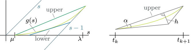
Figure 2: The left picture shows that we can approximate a monotone and convex function from below with linear functions. It furthermore shows the corridor in which the divergence will be located. Furthermore, there is a degree of freedom in choosing a tangential straight from below. A mirrored straight $g^{\prime\prime}$, which is a feasible lower bound yields the same convergence rate for the lower bound. The worse case that could happen for approximation is that the function has a kink as shown on the right picture. The right picture shows an interval $[t_{k},t_{k+1}]$. Then we see the error for the upper bound scales with the volume of a blunt triangle.

III Discussion

Solving (1) is an important problem in various areas in quantum information science, because it generally includes all types of optimisation which one can repatriate to the relative entropy, a central factor in information theory. However, for the general task and without any constraints on $\rho$ and $\sigma$ it is hopeless to get a good numerically tool set, because it is well known that the relative entropy diverges for cases of arbitrary small smallest eigenvalues of $\rho^{1/2}\sigma\rho^{1/2}$. Next to this physical challenge it is often hard to become provable lower bounds on magnitudes like the key rate in QKD scenarios. The challenge here is that convex optimisation methods frequently give good approximations to the optimal value but without guarantee that the value is e.g. a lower bound. However, for security of certain protocols exactly this property is unavoidable.

For the latter problem, the present method joins a list of already existent methods [17, 18, 19, 14, 20, 15, 16], which are mostly concerned with the application in key rate estimation. Roughly we can classify the methods so far into the three classes of interior point methods [17, 14], based on semi definite hierarchies [18, 20] and estimating the conditional entropy with the min-entropy [31]. The recently published follow up project [19] of [18] uses concrete hierarchies of semi definite optimisation with characterised devices. Importantly this whole approach is based on an integral representation of the relative entropy respective the logarithm as well but uses different techniques for the integration. We summarise the existing methods in Table 1. However, we can summarise in fairness that the final representation of the optimisation program in our approach convinces with outstanding simplicity.

In comparison to each of the already existent methods we give a toolbox for provable upper and lower bounds and a convergence result for compact intervals $[\mu,\lambda]$ with $\mu>0$. However, assuming $\mu=0$ is practical manageable as discussed in Appendix F as well. The fact that we need fixed integral bounds $0<\mu\leq\lambda$ which on first view seems to be a disadvantage, turns out to be the important ingredient for a rigorous numerical analysis. The existence of these values bounds the problem to finite range and one can think about the lower respective upper bounds as continuous functionals with values in a compact set. Therefore a rigorous numerical analysis becomes applicable. It is a beautiful observation that compactness of the image of the functionals is equivalent to finite relative entropy. Since we are only interested in minimisation tasks here, we get rid of numerical analysis artifacts with infinities directly and naturally.

In contrast, controlling the number and places of supporting points is in general a difficult game with no a priori best solution. Of course one has to have in mind that practically the number of grid points must not be too big, because it increases the number of variables in the SDP solver directly. This calls for a clever heuristic, especially with regard to even larger dimensions. With the proofs of Proposition 2 and Corollary 1 we give a clear mathematical, and therefore rigorous, framework which one can use in constructing heuristics. E.g. the fact that one can get rid of the $\mu$-dependence from Proposition 2 to Corollary 1 yields a good intuition for a heuristic: there should be unequal weighted number of grid points close to $\mu$ and close to $\lambda$. Another key could be to design a method that removes grid points as well. Many scenarios are possible here, which we leave open for future adjustment. In addition to heuristics, we would like to mention that our approach can also be carried out directly with the original integral representation of Frenkel [1]. Since the singularities at $0$ and $1$ play a decisive role there, it becomes much more difficult to extract provable scenarios. However, we did numerical experiments in this direction with success, but apparently without numerical analysis.

Concluding these thoughts, they open up different avenues for future research with the methods outlined here. On the one hand, a big but important challenge is to develop a heuristic that underpins the theoretical results that few grid points are sufficient. On the other hand one can apply the methods to different problem instances which are related to the relative entropy. The simplest one would be an optimisation over the von Neumann entropy under linear constraints. Lastly and concretely for the QKD application, one can start a straightforward improvement to a device independent algorithm. For this purpose one can use the ideas of [32]. Here one starts with a $C^{\star}$-algebra to be the quantum system one is considering. In each level of the hierarchy one gets the nonlinear optimisation task (11) for a fixed dimension, which one can relax to (6) and (8) with the positivity constraints coming from the postive cone $\Sigma_{2}$ in [32]. The positivity conditions in (6) and (8) translate directly from positvity conditions of $\Sigma_{2}^{\star}$ in each step in [32].

Similarly one could directly combine our approach with the seminal DPS [33] hierarchy for optimising in one argument in the set of separable states. As outlined in Appendix I, combining these methods gives lower bounds on e.g. the relative entropy of entanglement in a very natural way.

IV Methods

We divide this section into two parts, namely the analysis of $\operatorname{tr}^{+}[\sigma s-\rho]$, which becomes a central ingredient in our convergence analysis and the convergence analysis itself then becomes the second part of this section.

– Analysis of $\operatorname{tr}^{+}[\sigma s-\rho]$ :

Our method for the relaxations in (6) and (8) is based on the following observation. Consider $\rho,\sigma\in\mathcal{S}(\mathcal{H})$ with $\mu\sigma\leq\rho\leq\lambda\rho$. Then we have

$$D(\rho\parallel\sigma)-\log\lambda-1+\lambda =\int_{\mu}^{\lambda}\frac{ds}{s}\operatorname{tr}^{+}[\sigma s-\rho]$$ (12)

$$=\int_{\mu}^{\lambda}\frac{ds}{s}\sup_{0\leq P\leq\mathds{1}}\operatorname{tr}[P(\sigma s-\rho)].$$

At this point, we would evaluate the supremum in $P$ for each point $s\in[\mu,\lambda]$. Therefore it is valid to estimate the evaluation of the supremum once a time after integration

$$\int_{\mu}^{\lambda}\frac{ds}{s}\sup_{0\leq P\leq\mathds{1}}\operatorname{tr}[P(\sigma s-\rho)]\geq\sup_{0\leq P\leq\mathds{1}}\int_{\mu}^{\lambda}\frac{ds}{s}\operatorname{tr}[P(\sigma s-\rho)].$$

Concluding this thought, the interpretation is that we choose the best linear function lower bounding the trace term in terms of approximating the integral and not the function $\operatorname{tr}^{+}[\sigma s-\rho]$ itself. Therefore we reinterpret the supremum from a pointwise given one to an optimum over integral values. In addition, we are using the formidable properties of $\operatorname{tr}^{+}[\sigma s-\rho]$ coming from the next Lemma 1.

Lemma 1 (Properties of Divergence).

Let $\rho,\sigma\in\mathcal{S}(\mathcal{H})$ be two quantum states. Then $g(s):=\operatorname{tr}^{+}[\sigma s-\rho]$ has the following properties

1. $g$ is convex for $s\in\mathbb{R}$ and in particular continuous

2. $g$ is monotonically increasing.

3. $\operatorname{tr}^{+}[\sigma s-\rho]$ satisfies the data processing inequality and asymptotically we have $s-1\leq\operatorname{tr}^{+}[\sigma s-\rho]\leq s$.

Proof.

Appendix C. ∎

Combining the facts that $\operatorname{tr}^{+}[\sigma s-\rho]$ is convex, monotonically increasing and that the interchange of integration and supremum gives valuable lower bounds yields even heuristically that a rare number of grid points is already enough for lower bounds on key rates. This implies particularly that for a situation where convergence of the relative entropy is in terms of computational resources out of scope, this approach nevertheless gives perhaps a lower bound on e.g. extractable randomness.

In Figure 2 we sketch $\operatorname{tr}^{+}[\sigma s-\rho]$ and what happens if one changes integral and supremum. For the convergence analysis we have a degree of freedom in the straight below of $\operatorname{tr}^{+}[\sigma s-\rho]$. We use this degree of freedom to optimise in integral norm as discussed above. For completeness we give in the proof of Proposition 1 a full derivation of formula (6). In contrast to the lower bound, the upper bound (8) becomes a straight forward procedure for estimating convex functions. In Appendix E is a derivation of (8) as well.

– Deatailed Convergence Analysis :

From Figure 2 it is geometrically immediate that the optimised lower bound on each interval has an error which is less than the error of the upper bound, i.e. a simple convexity argument that the mirrored straight $g^{\prime\prime}$ is a feasible straight as lower bound in (6) and get the same results in terms of complexities. Thus, we are left with proving the convergence for the upper bound.

We know that $\operatorname{tr}^{+}[\sigma s-\rho]$ is monotonically increasing and convex as proposed in Lemma 1 $(1)$ and $(2)$. For the convergence, we choose a grid $\mu=t_{1}\leq\cdots\leq t_{r}=\lambda$. For each subinterval we do a worst-case estimation in the sense that we relax $\operatorname{tr}^{+}[\sigma s-\rho]$ to the piecewise-defined function $g_{2}(s)$ and $g_{3}(s)$ which has one kink in $[t_{k},t_{k+1}]$ and the error grows with this estimate. The upper error is now given by $g^{\prime}\cdot h/2$ which scales like $\delta^{2}\tan(\alpha)$. From Lemma 1 $(4)$ we know that the tangent, $\tan(\alpha)$, is bounded by the largest gradient, $1$ as shown in Lemma 1 $(3)$ and the fact that $\operatorname{tr}^{+}[\sigma s-\rho]$ is monotonically increasing. Therefore, as outlined in Appendix D, we are left with a telescopic sum over gradients, which becomes $1$ and thus finishes the proof.

V Acknowledgements

We thank Mario Berta, Tobias J. Osborne, Hermann Kampermann, Martin Plavala and Zhen-Peng Xu for helpful discussions around the topic. We thank Omar Fawzi for pointing us to the reference [15] from which we took the examples in Appendix H. GK thanks especially MB for many discussions with hints and possible extensions. RS acknowledges support from the Quantum Valley Lower Saxony and the Quantum Frontiers cluster of excellence. RS acknowledges financial support from the BMBF projects ATIQ and CBQD.

Appendix A Discussion about Instances

In the first plot of Figure 1 we consider a generic random pair of states $\rho$ and $\sigma$ and test Corollary 1. Therefore we aim to estimate the relative entropy between the two states. As shown, we have convergence as proposed and even the constant factor is there approximately $c\approx\lambda$. Therefore we conclude that Corollary 1 is close to optimal from the theoretical perspective.

In the middle we see a generic problem for the full problem statement. As shown, we have even there quadratic convergence and get the proposed value with guarantee due to the fact that we can bound from below and above.

The right plot describes the usual instance used in QKD protocols with mutually unbiased bases in each dimension and the question about the lower bound on the key rate. Even there, whereby the problem has dimension $64$, we get good convergence results for each parameter of $\alpha$. For this purpose we consider a maximally entangled state $\Omega^{+}$ in different dimensions and mix it with white noise depending on a parameter $\alpha\in[0,1]$

$$\Omega(\alpha):=(1-\alpha)\Omega^{+}+\alpha\frac{\mathds{1}}{d^{2}}.$$

Figure 1 shows now solutions for different fixed values of $\alpha\in[0,1]$ of (11), whereby the measurement channels are constructed with two mutually unbiased basis. We executed the algorithm for the local dimensions two, four and eight of Alice, respective Bob’s system. As a result we get the well known lower bounding curves for the Devetak-Winter estimate as shown in Figure 1.

From a numerical perspective one can use Hayashi’s pinching inequality [34] to estimate the expected number of grid points in Corollary 1. Du to the fact that $\lambda=\sqrt{d}$, for $d$, the dimension of the global system, we can estimate the number of grid points with $\frac{d^{1/4}}{\sqrt{\varepsilon}}$ for an $\varepsilon$-approximation. This yields that in this particular case the number of grid points becomes dimension dependent, but for reasonable settings negligible, because even for local dimension $16$ this would yield $d^{1/4}=4$. Therefore the global system size and the state of the art SDP solver would lead firstly to a runtime challenge until we have an inapplicable number of grid points due to the estimate in Corollary 1.

Appendix B Proof of Proposition 1

The first statement follows from the following calculation. Let $\mu=t_{1}\leq\cdots\leq t_{r}=\lambda$. Then we have

$$\int_{\mu}^{\lambda}\frac{ds}{s}\operatorname{tr}^{+}[\sigma s-\rho] =\sum_{k=1}^{r-1}\int_{t_{k}}^{t_{k+1}}\frac{ds}{s}\sup_{0\leq P\leq\mathds{1}}\operatorname{tr}[P(\sigma s-\rho)]$$

$$\geq\sum_{k=1}^{r-1}\sup_{0\leq P\leq\mathds{1}}\int_{t_{k}}^{t_{k+1}}\frac{ds}{s}\operatorname{tr}[P(\sigma s-\rho)]$$

$$=\sum_{k=1}^{r-1}\sup_{0\leq P\leq\mathds{1}}\operatorname{tr}[P\sigma]\underbrace{(t_{k+1}-t_{k})}_{=:\beta_{k}}\ +$$

$$\quad\quad\quad\quad\quad\quad\quad\operatorname{tr}[P\rho]\underbrace{\log\frac{t_{k}}{t_{k+1}}}_{=:\alpha_{k}}$$

$$=\sum_{k=1}^{r-1}\sup_{0\leq P\leq\mathds{1}}\operatorname{tr}[P(\sigma\beta_{k}+\rho\alpha_{k})]$$

$$=\inf_{\mu_{1},\ldots,\mu_{r-1}}\sum_{k=1}^{r-1}\operatorname{tr}[\mu_{k}]$$

$$\quad\quad\text{s.th.}\ \mu_{k}\geq\alpha_{k}\rho+\beta_{k}\sigma.$$

This gives us (6).

Appendix C Proof of Lemma 1

– Convexity and Continuity:

The convexity follows by the following calculation similar to [35]

$$\operatorname{tr}^{+}[\sigma(\lambda s_{1}+(1-\lambda)s_{2})-\rho] =\operatorname{tr}^{+}[\lambda(\sigma s_{1}-\rho)+(1-\lambda)(\sigma s_{2}-\rho)]$$

$$=\sup_{0\leq P\leq\mathds{1}}\lambda\operatorname{tr}[P(\sigma s_{1}-\rho)]+(1-\lambda)\operatorname{tr}[P(\sigma s_{2}-\rho)]$$

$$\leq\lambda\sup_{0\leq P\leq\mathds{1}}\operatorname{tr}[P(\sigma s_{1}-\rho)]+(1-\lambda)\sup_{0\leq P\leq\mathds{1}}\operatorname{tr}[P(\sigma s_{2}-\rho)]$$

$$=\lambda\operatorname{tr}^{+}[\sigma s_{1}-\rho]+(1-\lambda)\operatorname{tr}^{+}[\sigma s_{2}-\rho].$$

For continuity let $\rho,\tilde{\rho},\sigma,\tilde{\sigma}$ be quantum states and $s_{1},s_{2}\in\mathbb{R}_{\geq 0}$. Then we have similar to [36]

$$2\cdot|\operatorname{tr}^{+}[\sigma s_{1}-\rho]-\operatorname{tr}^{+}[\tilde{\sigma}s_{2}-\tilde{\rho}]| =|\|s_{1}\sigma-\rho\|_{1}+(s_{1}-1)-(\|\tilde{\sigma}s_{2}-\tilde{\rho}\|_{1}+s_{2}-1)|$$

$$\leq|s_{2}-s_{1}|+\|\rho-\tilde{\rho}\|_{1}+\|s_{1}\sigma-s_{2}\tilde{\sigma}\|_{1}.$$

whereby we used the reversed triangle inequality for the one-norm. In particular we see that the divergence is continuous in the states. In the other way around for equal states and different $s_{1/2}$ we have continuity in $s$.
– Monotony:  The monotony is a direct consequence of the fact that for $s_{1}\geq s_{2}$ we have

$$\sigma s_{1}-\rho\geq\sigma s_{2}-\rho.$$

– Asymptotic Behaviour:

Consider a channel $\Phi:\mathcal{B}_{1}(\mathcal{H})\to\mathcal{B}_{1}(\mathcal{H})$. We assume that $D_{\text{max}}(\rho\parallel\sigma)<\infty$ and satisfies the data processing inequality. This yields that $D(\rho\parallel\sigma)-D(\Phi(\rho)\parallel\Phi(\sigma))$ is a finite number. Adapting from [36, Lemmma 4] the proof that $\operatorname{tr}^{+}[\sigma s-\rho]$ satisfies the data processing inequality, namely let $\sigma s-\rho=Q-S$ with $Q,S\geq 0$. Then let $P:=P_{\Phi(\sigma)s-\Phi(\rho)\geq 0}$ and

$$\operatorname{tr}^{+}[\sigma s-\rho] =\operatorname{tr}[Q]$$

$$=\operatorname{tr}[\Phi(Q)]$$

$$\geq\operatorname{tr}[P(\Phi(Q)-\Phi(S))]$$

$$=\operatorname{tr}[P(\Phi(\sigma s-\rho)]$$

$$=\operatorname{tr}^{+}[\Phi(\sigma)s-\Phi(\rho)].$$

Therefore we know that for any $\kappa\geq\lambda$

$$0 =\int_{\lambda}^{\kappa}\frac{ds}{s}\underbrace{\operatorname{tr}^{+}[\sigma s-\rho]-\operatorname{tr}^{+}[\Phi(\sigma)s-\Phi(\rho)]}_{\geq 0}$$

$$=\int_{\lambda}^{\kappa}\frac{ds}{s}|\operatorname{tr}^{+}[\sigma s-\rho]-\operatorname{tr}^{+}[\Phi(\sigma)s-\Phi(\rho)]|.$$

The property now follows from the fact that $\|\cdot\|_{1}$ is a norm on the space of integrable functions and we know easily that every classical dichotomy of states satisfies the property asymptotically and the fact that channels are trace preserving.

Appendix D Proof of Proposition 2 and Corollary 1

Lemma 2.

Let $f$ be a convex and monotonically increasing function and $\mu=t_{1}\leq\ldots\leq t_{r}=\lambda$ be a grid. Then the Trapezoid rule satisfies the error estimate

$$|I(f)-T(f)|\leq\frac{1}{2}M\delta^{2}$$

with a maximal grid size $\delta$ and a maximal upper bound on the subgradients $M$.

Proof.

This is an easy geometric consequence. One has to include that the error of the integral on each subinterval does only depend on the difference of the gradient leaving the interval minus the gradient coming into the interval. But, as shown in Figure 2, the resulting triangle is always a blunt triangle. ∎

Using Lemma 2 we see that the convergence rate is immediate with Hölder’s inequality under the integral with $p=\infty$ and $q=1$. Moreover the supremum of $1/s$ is bounded by $1/\mu$. The gradient in Lemma 2 can be estimated with $1$ coming from Lemma 1 $(4)$. With these information the rate $O(\frac{\mu}{d}\delta^{2})$ is clear. The other statements are straightforward calculations as we can estimate for a uniform grid the number of grid points with $O((\lambda-\mu)\sqrt{\frac{d}{\mu\varepsilon}})$.

Proof of the Corollary: It is easy to see that if we consider the three straights

$$g_{1}(s) =\frac{m_{1}+m_{2}}{p+q}s$$

$$g_{2}(s) =\frac{m_{1}}{p}s$$

$$g_{3}(s) =\frac{m_{2}}{q}(s-p)+m_{1}$$

the following inequality holds

$$\int_{0}^{p+q}g_{1}(s)ds- \int_{0}^{p}g_{2}(s)ds-\int_{p}^{p+q}g_{3}(s)ds$$

$$\leq\frac{1}{2}(\frac{m_{2}}{q}-\frac{m_{1}}{p})pq.$$

This means that the error depends only on the gradient leaving the interval $[0,p+q]$ minus the gradient coming in the interval, if we aim to approximate a convex and monotone function with a linear function. Estimating $p\cdot q\leq\frac{1}{4}\delta^{2}$ yields the convergence in terms of $\delta$.

In a second step we can divide an interval starting in $t_{k}$ in steps with step size $\delta(t_{k})=\sqrt{8t_{k}\varepsilon}$. This leads to the recursive formula

$$t_{k}=t_{k-1}+\sqrt{8t_{k-1}\varepsilon}.$$

With this adapted $\delta(t_{k})>0$ we can estimate

$$|\int_{\mu}^{\lambda}\frac{ds}{s}\operatorname{tr}^{+}[\sigma s-\rho]-T(f)| =\sum_{k=1}^{r-1}\int_{t_{k}}^{t_{k+1}}\frac{ds}{s}|\operatorname{tr}^{+}[\sigma s-\rho]-g^{(k)}_{1}(s)|$$

$$\leq\sum_{i=1}^{r-1}\sup_{s\in[t_{k(i)},t_{k(i)+1}]}|\frac{1}{s}|\int_{t_{k(i)}}^{t_{k(i)+1}}ds|\operatorname{tr}^{+}[\sigma s-\rho]-g^{(k)}_{1}(s)|$$

$$\leq\sum_{i=1}^{r-1}\frac{1}{t_{k(i)}}\frac{1}{8}(\tilde{m}_{i+1}-\tilde{m}_{i})\delta^{2}(t_{k(i)})$$

$$\leq\sum_{i=1}^{r-1}\frac{1}{t_{k(i)}}\frac{1}{8}(\tilde{m}_{i+1}-\tilde{m}_{i})8t_{k(i)}\varepsilon$$

$$=\varepsilon\sum_{i=1}^{r-1}(\tilde{m}_{i+1}-\tilde{m}_{i})$$

$$=\varepsilon.$$

We used in step two Hölder’s inequality and in the last step the fact that asymptotically the function $\operatorname{tr}^{+}[\sigma s-\rho]$ has gradient equal to $1$ from Lemma 1 and $\tilde{m}_{0}=0$, because we assumed $\mu>0$.
We are left with the task to estimate the number of grid points for the dependent $\delta(t_{k})$. For this purpose we have to find a function $f:\mathbb{N}\to\mathbb{R}$ such that

$$f(k)\leq f(k-1)+\sqrt{8f(k-1)\varepsilon}$$

and $f(0)=\mu$. It is easy to see that $f(k)=(\frac{\sqrt{\varepsilon}}{2}k+\sqrt{\mu})^{2}$ does it if $\varepsilon<\mu$. Therefore we need at most

$$f(k) \leq\lambda\quad\Leftrightarrow$$

$$k \leq\frac{\sqrt{2\lambda}-\sqrt{2\mu}}{\sqrt{\varepsilon}}$$

$$k \leq\sqrt{\frac{2\lambda}{\varepsilon}}$$

grid points for an $\varepsilon$-approximation.

Appendix E Derivation Upper Bound

Choose a grid $\mu=t_{1}\leq\cdots\leq t_{r}=\lambda$ and define

$$y_{k}:=\sup_{0\leq P\leq\mathds{1}}\operatorname{tr}[P(\sigma t_{k}-\rho)]$$

Then we have due to the convexity of $\operatorname{tr}^{+}[\sigma s-\rho]$

$$\int_{\mu}^{\lambda}\frac{ds}{s}\operatorname{tr}^{+}[\sigma s-\rho] =\sum_{k=1}^{r-1}\int_{t_{k}}^{t_{k+1}}\frac{ds}{s}\operatorname{tr}^{+}[\sigma s-\rho]$$

$$\leq\sum_{k=1}^{r-1}\int_{t_{k}}^{t_{k+1}}\frac{ds}{s}(\frac{y_{k+1}-y_{k}}{t_{k+1}-t_{k}}(s-t_{k})+y_{k})$$

$$=\sum_{k=1}^{r-1}(y_{k+1}-y_{k})\ +(y_{k}-t_{k}\frac{y_{k+1}-y_{k}}{t_{k+1}-t_{k}})\log\frac{t_{k+1}}{t_{k}}$$

$$=\sum_{k=1}^{r-1}y_{k+1}-t_{k}\frac{y_{k+1}}{t_{k+1}-t_{k}}\log\frac{t_{k+1}}{t_{k}}+\sum_{k=1}^{r-1}(y_{k}+\frac{t_{k}y_{k}}{t_{k+1}-t_{k}})\log\frac{t_{k+1}}{t_{k}}-y_{k}$$

$$=(y_{1}+\frac{t_{1}y_{1}}{t_{2}-t_{1}})\log\frac{t_{2}}{t_{1}}-y_{1}+y_{r}-\frac{t_{r-1}y_{r}}{t_{r}-t_{r-1}}\log\frac{t_{r}}{t_{r-1}}+\sum_{k=1}^{r-2}y_{k+1}-t_{k}\frac{y_{k+1}}{t_{k+1}-t_{k}}\log\frac{t_{k+1}}{t_{k}}$$

$$\quad+\sum_{k=2}^{r-1}(y_{k}+\frac{t_{k}y_{k}}{t_{k+1}-t_{k}})\log\frac{t_{k+1}}{t_{k}}-y_{k}$$

$$=(y_{1}+\frac{t_{1}y_{1}}{t_{2}-t_{1}})\log\frac{t_{2}}{t_{1}}-y_{1}+y_{r}-\frac{t_{r-1}y_{r}}{t_{r}-t_{r-1}}\log\frac{t_{r}}{t_{r-1}}+\sum_{k=2}^{r-1}\cancel{y_{k}}-t_{k-1}\frac{y_{k}}{t_{k}-t_{k-1}}\log\frac{t_{k}}{t_{k-1}}$$

$$\quad+\sum_{k=2}^{r-1}(y_{k}+\frac{t_{k}y_{k}}{t_{k+1}-t_{k}})\log\frac{t_{k+1}}{t_{k}}\cancel{-y_{k}}$$

$$=y_{1}[(1+\frac{t_{1}}{t_{2}-t_{1}})\log\frac{t_{2}}{t_{1}}-1]+y_{r}[1-\frac{t_{r-1}}{t_{r}-t_{r-1}}\log\frac{t_{r}}{t_{r-1}}]$$

$$\quad+\sum_{k=2}^{r-1}y_{k}[(1+\frac{t_{k}}{t_{k+1}-t_{k}})\log\frac{t_{k+1}}{t_{k}}-\frac{t_{k-1}}{t_{k}-t_{k-1}}\log\frac{t_{k}}{t_{k-1}}].$$

Inserting the definition of $y_{k}$ yields the following definitions for $\alpha_{k}$ and $\beta_{k}$

$$\delta_{k}=\begin{cases}[(1+\frac{t_{1}}{t_{2}-t_{1}})\log\frac{t_{2}}{t_{1}}-1]\cdot t_{1}&k=1\\ [1-\frac{t_{r-1}}{t_{r}-t_{r-1}}\log\frac{t_{r}}{t_{r-1}}]\cdot t_{r}&k=r\\ [(1+\frac{t_{k}}{t_{k+1}-t_{k}})\log\frac{t_{k+1}}{t_{k}}-\frac{t_{k-1}}{t_{k}-t_{k-1}}\log\frac{t_{k}}{t_{k-1}}]\cdot t_{k}&\text{else}.\end{cases}$$

and for $\delta_{k}$

$$\gamma_{k}=\begin{cases}-[(1+\frac{t_{1}}{t_{2}-t_{1}})\log\frac{t_{2}}{t_{1}}-1]&k=1\\ -[1-\frac{t_{r-1}}{t_{r}-t_{r-1}}\log\frac{t_{r}}{t_{r-1}}]&k=r\\ -[(1+\frac{t_{k}}{t_{k+1}-t_{k}})\log\frac{t_{k+1}}{t_{k}}-\frac{t_{k-1}}{t_{k}-t_{k-1}}\log\frac{t_{k}}{t_{k-1}}]&\text{else}.\end{cases}$$

Thus we conclude

$$\int_{\mu}^{\lambda}\frac{ds}{s}\operatorname{tr}^{+}[\sigma s-\rho] \leq\sum_{k=1}^{r}\sup_{0\leq P\leq\mathds{1}}\operatorname{tr}[P(\gamma_{k}\rho+\delta_{k}\sigma)]$$ (13)

$$=\inf_{\nu_{1},\ldots,\nu_{r}}\sum_{k=1}^{r}\operatorname{tr}[\nu_{k}]$$ (14)

$$\quad\quad\text{s.th.}\ \nu_{k}\geq\gamma_{k}\rho+\delta_{k}\sigma.$$ (15)

Appendix F Discussion about $\mu=0$

In applications it is possible that $\mu$, the lower bound in the integral representation becomes zero. Our theoretical results can not apply due to the weight function $1/s$ even though the integral representation is finite anyway. However, from an experimental point of view coming from reality we can always assume that all states considered have a bit white noise such that $\mu$ is strictly greater than zero. From a mathematical perspective, however, this is unsatisfactory. Therefore we provide a practical way out, which will not affect our results up to a small error. First of all we observe that a finite $\lambda>0$ for a dichotomy of states $(\rho,\sigma)$ implies $\ker\sigma\subset\ker\rho$ immediately. This shows that the difficult part of numerical analysis with the relative entropy is exactly classified in terms of $\lambda\to\infty$. In particular, as we saw, quantum crytography behaves in these terms very formidable. Otherwise the case $\mu>0$ implies $\ker\sigma=\ker\rho$ which is manageable in a straight forward manner of our discussion. We are left with the situation $\ker\sigma\subsetneq\ker\rho$. In this case $\mu$ becomes zero. But interestingly we can estimate the first step with an estimate which becomes tight for a grid tending to zero. For this purpose we consider a grid $\mu=t_{0}<t_{1}<\ldots<t_{n}=\lambda$. Between $t_{1}$ and $t_{n}$ the whole story from above is applicable. Only on the interval $[t_{0},t_{1}]$ we replace

$$\int_{0}^{t_{1}}\frac{ds}{s}\operatorname{tr}^{+}[\sigma s-\rho] \geq\int_{0}^{t_{1}}\frac{ds}{s}\operatorname{tr}[P_{(\ker\rho)}(\sigma s-\rho)]$$

$$=\operatorname{tr}[P_{(\ker\rho)}\sigma]\int_{0}^{t_{1}}ds$$

with $P_{(\ker\rho)}$ is a solution to $\sup_{0\leq P\leq\mathds{1}}\operatorname{tr}[P(\mathds{1}-\rho)]$. That this estimate is a lower bound follows immediately. Moreover it becomes tight in the case of $t_{1}$ small enough.

Appendix G SDP formulations for Standard Task

The method presented here is able to solve tasks which have one of the following properties

1. It is a minimisation over a positive weighted sum of relative entropies

   $$\text{min}\sum_{i}\zeta_{i} D(\rho^{(i)}\parallel\sigma^{(i)})$$

   s.th. semi definite constraints on the states

   i.e. $\zeta_{i}\geq 0$ for all $i$

2. each state within each relative entropy is linear in the sdp variables, i.e. something like $\rho^{(i)}=\Phi(\tilde{\rho}^{(i)})$ whereby $\tilde{\rho}^{(i)}$ is the actual SDP variable. Exemplary $\Phi$ could be the channel that tensorises just a state or a measurement.

Therefore we can estimate sums of e.g. the following summands

1. For the entropy of a state $\rho$ under linear constraints we can maximise $H(\rho)=\log d-D(\rho\parallel\mathds{1}/d)$ under linear constraints if we equivalently minimise

   $$\begin{aligned} \inf_{\rho}\ &D(\rho\parallel\mathds{1}/d)\\ \text{s.th.}&\ \;h_{i}(\rho)\geq 0\quad i=1,\dots,n\\ &\mu\mathds{1}\leq\rho\leq\lambda\mathds{1}\\ &\rho\in\mathcal{S}(\mathcal{H})\end{aligned}\qquad\Rightarrow\qquad\begin{aligned} \inf_{\rho,\nu_{k}}&\sum_{k}\operatorname{tr}[\nu_{k}]+\log\lambda+1-\lambda\\ \text{s.th.}&\ \;h_{i}(\rho)\geq 0\quad i=1,\dots,n\\ &\nu_{k}\geq\gamma_{k}\rho+\delta_{k}\mathds{1}\quad\forall k\\ &\mu\mathds{1}\leq\rho\leq\lambda\mathds{1}\\ &\rho\in\mathcal{S}(\mathcal{H})\quad\nu_{k}\geq 0\end{aligned}$$

2. For the conditional entropy of a state $\rho$ under linear constraints we can maximise

   $$H(A|B)_{\rho_{AB}}=\log d_{A}-D(\rho_{AB}\parallel\mathds{1}_{A}/d_{A}\otimes\rho_{B})$$

   under linear constraints if we equivalently minimise

   $$\begin{aligned} \inf_{\rho}\ &D(\rho_{AB}\parallel\mathds{1}/d_{A}\otimes\rho_{B})\\ \text{s.th.}&\ \;h_{i}(\rho_{AB})\geq 0\quad i=1,\dots,n\\ &\mu\mathds{1}/d_{A}\otimes\rho_{B}\leq\rho_{AB}\leq\lambda\mathds{1}/d_{A}\otimes\rho_{B}\\ &\rho_{AB}\in\mathcal{S}(\mathcal{H}_{A}\otimes\mathcal{H}_{B})\end{aligned}\qquad\Rightarrow\qquad\begin{aligned} \inf_{\rho,\nu_{k}}&\sum_{k}\operatorname{tr}[\nu_{k}]+\log\lambda+1-\lambda\\ \text{s.th.}&\ \;h_{i}(\rho_{AB})\geq 0\quad i=1,\dots,n\\ &\mu\mathds{1}/d_{A}\otimes\rho_{B}\leq\rho_{AB}\leq\lambda\mathds{1}/d_{A}\otimes\rho_{B}\\ &\rho_{AB}\in\mathcal{S}(\mathcal{H}_{A}\otimes\mathcal{H}_{B})\quad\nu_{k}\geq 0.\end{aligned}$$

Appendix H Exemplary Application in Quantum Shannon Theory

We consider exemplary the task of calculating the entanglement-assisted classical capacity similar to [15, 3.2] of the amplitude damping channel. This section is intended to demonstrate the strength and diversity of our approach rather than to maximising out its numerical limitations.

We consider the amplitude damping channel in its basic form with Kraus-representation

$$K_{1}:=\begin{pmatrix}1&0\\ 0&\sqrt{1-p}\end{pmatrix}\quad K_{2}:=\begin{pmatrix}0&\sqrt{p}\\ 0&0.\end{pmatrix}$$

As shown in the repository it is easy to find an isometry that implements the dilation $U$ of the amplitude channel. Reference [37] has shown that the entanglement-assisted classical capacity can be formulated as the following optimisation task

$$C(\mathcal{A}_{p}):=\max_{\sigma\in\mathcal{S}(\mathcal{H})}I(\sigma,\mathcal{A}_{p}),$$

whereby $\mathcal{A}_{p}$ is the amplitude damping channel with damping parameter $p$ and $I$ the mutual information. For our specific case, this yields

$$I(\sigma,\mathcal{A}_{p})=H(B|E)_{U\sigma U^{\dagger}}+H(B)_{U\sigma U^{\dagger}}.$$

Particularly we can rewrite this expression for $\rho_{BE}:=U\sigma U^{\dagger}$ to be

$$I(\rho_{BE},\mathcal{A}_{p})=\log(d_{B}^{2})-D(\rho_{BE}\parallel\mathds{1}_{B}/d_{B}\otimes\rho_{E})-D(\rho_{B}\parallel\mathds{1}_{B}/d_{B}).$$

That means optimising $I$ is equivalent to minimising

$$\min_{\rho=U\sigma U^{\dagger}}D(\rho_{BE}\parallel\mathds{1}_{B}/d_{B}\otimes\rho_{E})+D(\rho_{B}\parallel\mathds{1}_{B}/d_{B}).$$

This problem can be easily implemented if we just add our approach two times from (6) and (8) with two sets of variables $\tau$ but just one $\rho$.

Figure 3: The plot shows exemplarily the entanglement assisted capacity of the amplitude damping channel on a qubit in dependence of the damping parameter. The plot is similar to figure 1 in [15].

Appendix I Entanglement Measures

This section is devoted to a ”proof-of-principle” of our technique for estimating entanglement measures. We aim to estimate for a fixed $\rho_{AB}\in\mathcal{S}(\mathcal{H}_{A}\otimes\mathcal{H}_{B})$ the following optimisation problem

$$\min_{\sigma_{AB}\in\text{SEP}(A:B)}D(\rho_{AB}\parallel\sigma_{AB}).$$ (16)

We denote to be $\text{SEP}(A:B)$ to be the set of all separable states over the bipartition $\mathcal{H}_{A}\otimes\mathcal{H}_{B}$. The quantity in (16) is often called relative entropy of entanglement [38] and has a significant meaning in entanglement theory (see e.g. [39]). For general Hilbert spaces even the membership problem for the set of separable states a NP-hard problem [40].

Nevertheless, there are SDP-hierarchies to solve (16) if the functional would be a usual linear SDP [33, 41]. Combining our linearisation and a hierarchy for the set of separable states could therefore yield reasonable lower bounds (the hierarchies are optimising over e.g. $n$-extendable states and therefore relax the problem in terms of lower bounds and we are providing in particular lower bounds as well).

We would like to repeat that the aim of this appendix is not to exhaust the numerical possibilities, but rather to demonstrate the versatility of our approach by way of example. Thus, we use the fact that for two qubits the PPT criterium is sufficient [42] and show the relative entropy of entanglement for an entangled state on two qubits mixed with white noise.

Figure 4: The plot shows the relative entropy of entanglement on a pair of qubits here with PPT criterium in dependence with a maximally entangled state mixed with white noise. The amount of white noise is calculated with a parameter alpha.

References

- Frenkel [2023] P. E. Frenkel, Integral formula for quantum relative entropy implies data processing inequality, Quantum 7, 1102 (2023).
- Bennett and Brassard [2014] C. H. Bennett and G. Brassard, Quantum cryptography: Public key distribution and coin tossing, Theoretical computer science 560, 7 (2014).
- Pirandola et al. [2020] S. Pirandola, U. L. Andersen, L. Banchi, M. Berta, D. Bunandar, R. Colbeck, D. Englund, T. Gehring, C. Lupo, C. Ottaviani, et al., Advances in quantum cryptography, Advances in optics and photonics 12, 1012 (2020).
- Nadlinger et al. [2022] D. P. Nadlinger, P. Drmota, B. C. Nichol, G. Araneda, D. Main, R. Srinivas, D. M. Lucas, C. J. Ballance, K. Ivanov, E. Y.-Z. Tan, P. Sekatski, R. L. Urbanke, R. Renner, N. Sangouard, and J.-D. Bancal, Experimental quantum key distribution certified by bell's theorem, Nature 607, 682 (2022).
- Zhang et al. [2022] W. Zhang, T. van Leent, K. Redeker, R. Garthoff, R. Schwonnek, F. Fertig, S. Eppelt, W. Rosenfeld, V. Scarani, C. C.-W. Lim, and H. Weinfurter, A device-independent quantum key distribution system for distant users, Nature 607, 687 (2022).
- Renner [2006] R. Renner, Security of quantum key distribution (2006), arXiv:quant-ph/0512258 [quant-ph] .
- Portmann and Renner [2022] C. Portmann and R. Renner, Security in quantum cryptography, Reviews of Modern Physics 94, 10.1103/revmodphys.94.025008 (2022).
- Dupuis et al. [2020] F. Dupuis, O. Fawzi, and R. Renner, Entropy accumulation, Communications in Mathematical Physics 379, 867 (2020).
- Arnon-Friedman et al. [2018] R. Arnon-Friedman, F. Dupuis, O. Fawzi, R. Renner, and T. Vidick, Practical device-independent quantum cryptography via entropy accumulation, Nature communications 9, 459 (2018).
- Metger and Renner [2023] T. Metger and R. Renner, Security of quantum key distribution from generalised entropy accumulation, Nature Communications 14, 5272 (2023).
- Tan et al. [2022] E. Y.-Z. Tan, P. Sekatski, J.-D. Bancal, R. Schwonnek, R. Renner, N. Sangouard, and C. C.-W. Lim, Improved diqkd protocols with finite-size analysis, Quantum 6, 880 (2022).
- Christandl et al. [2009a] M. Christandl, R. König, and R. Renner, Postselection technique for quantum channels with applications to quantum cryptography, Physical review letters 102, 020504 (2009a).
- Senno et al. [2023] G. Senno, T. Strohm, and A. Acín, Quantifying the intrinsic randomness of quantum measurements, Physical Review Letters 131, 10.1103/physrevlett.131.130202 (2023).
- Winick et al. [2018] A. Winick, N. Lütkenhaus, and P. J. Coles, Reliable numerical key rates for quantum key distribution, Quantum 2, 77 (2018).
- Fawzi and Fawzi [2018] H. Fawzi and O. Fawzi, Efficient optimization of the quantum relative entropy, Journal of Physics A: Mathematical and Theoretical 51, 154003 (2018).
- Fawzi et al. [2018] H. Fawzi, J. Saunderson, and P. A. Parrilo, Semidefinite approximations of the matrix logarithm, Foundations of Computational Mathematics 19, 259–296 (2018).
- Hu et al. [2022] H. Hu, J. Im, J. Lin, N. Lütkenhaus, and H. Wolkowicz, Robust interior point method for quantum key distribution rate computation, Quantum 6, 792 (2022).
- Brown et al. [2023] P. Brown, H. Fawzi, and O. Fawzi, Device-independent lower bounds on the conditional von neumann entropy (2023), arXiv:2106.13692 [quant-ph] .
- Araú jo et al. [2023] M. Araú jo, M. Huber, M. Navascués, M. Pivoluska, and A. Tavakoli, Quantum key distribution rates from semidefinite programming, Quantum 7, 1019 (2023).
- Tan et al. [2021] E. Y.-Z. Tan, R. Schwonnek, K. T. Goh, I. W. Primaatmaja, and C. C.-W. Lim, Computing secure key rates for quantum cryptography with untrusted devices, npj Quantum Information 7, 10.1038/s41534-021-00494-z (2021).
- Jenčová [2023] A. Jenčová, Recoverability of quantum channels via hypothesis testing (2023), arXiv:2303.11707 [quant-ph] .
- Hiai and Petz [1991] F. Hiai and D. Petz, The proper formula for relative entropy and its asymptotics in quantum probability, Communications in mathematical physics 143, 99 (1991).
- Augustino [2023] B. Augustino, Quantum algorithms for symmetric cones (2023).
- Devetak and Winter [2005] I. Devetak and A. Winter, Distillation of secret key and entanglement from quantum states, Proceedings of the Royal Society A: Mathematical, Physical and Engineering Sciences 461, 207 (2005).
- Tomamichel et al. [2009] M. Tomamichel, R. Colbeck, and R. Renner, A fully quantum asymptotic equipartition property, IEEE Transactions on Information Theory 55, 5840–5847 (2009).
- Renner and Cirac [2009] R. Renner and J. I. Cirac, de finetti representation theorem for infinite-dimensional quantum systems and applications to quantum cryptography, Physical Review Letters 102, 10.1103/physrevlett.102.110504 (2009).
- Christandl et al. [2009b] M. Christandl, R. König, and R. Renner, Postselection technique for quantum channels with applications to quantum cryptography, Physical review letters 102, 020504 (2009b).
- Arnon-Friedman and Renner [2015] R. Arnon-Friedman and R. Renner, de finetti reductions for correlations, Journal of Mathematical Physics 56, 052203 (2015).
- Tomamichel [2016] M. Tomamichel, Quantum Information Processing with Finite Resources (Springer International Publishing, 2016).
- Coles et al. [2016] P. J. Coles, E. M. Metodiev, and N. Lütkenhaus, Numerical approach for unstructured quantum key distribution, Nature communications 7, 11712 (2016).
- Konig et al. [2009] R. Konig, R. Renner, and C. Schaffner, The operational meaning of min- and max-entropy, IEEE Transactions on Information Theory 55, 4337 (2009).
- Koßmann et al. [2023] G. Koßmann, R. Schwonnek, and J. Steinberg, Hierarchies for semidefinite optimization in -algebras (2023), arXiv:2309.13966 [math.OC] .
- Doherty et al. [2005] A. C. Doherty, P. A. Parrilo, and F. M. Spedalieri, Detecting multipartite entanglement, Physical Review A 71, 10.1103/physreva.71.032333 (2005).
- Hayashi [2002] M. Hayashi, Optimal sequence of quantum measurements in the sense of stein s lemma in quantum hypothesis testing, Journal of Physics A: Mathematical and General 35, 10759–10773 (2002).
- Hirche et al. [2023] C. Hirche, C. Rouzé, and D. S. Franca, Quantum differential privacy: An information theory perspective (2023), arXiv:2202.10717 [quant-ph] .
- Sharma and Warsi [2013] N. Sharma and N. A. Warsi, Fundamental bound on the reliability of quantum information transmission, Physical Review Letters 110, 10.1103/physrevlett.110.080501 (2013).
- Bennett et al. [2002] C. H. Bennett, P. W. Shor, J. A. Smolin, and A. V. Thapliyal, Entanglement-assisted capacity of a quantum channel and the reverse shannon theorem (2002), arXiv:quant-ph/0106052 [quant-ph] .
- Piani [2009] M. Piani, Relative entropy of entanglement and restricted measurements, Physical Review Letters 103, 10.1103/physrevlett.103.160504 (2009).
- Berta and Tomamichel [2023] M. Berta and M. Tomamichel, Entanglement monogamy via multivariate trace inequalities (2023), arXiv:2304.14878 [quant-ph] .
- Gurvits [2002] L. Gurvits, Quantum matching theory (with new complexity theoretic, combinatorial and topological insights on the nature of the quantum entanglement) (2002), arXiv:quant-ph/0201022 [quant-ph] .
- Berta et al. [2021] M. Berta, F. Borderi, O. Fawzi, and V. B. Scholz, Semidefinite programming hierarchies for constrained bilinear optimization, Mathematical Programming 194, 781–829 (2021).
- Horodecki et al. [1996] M. Horodecki, P. Horodecki, and R. Horodecki, Separability of mixed states: necessary and sufficient conditions, Physics Letters A 223, 1–8 (1996).