The TruEnd-procedure: Treating trailing zero-valued balances in credit data

Abstract

A novel procedure is presented for finding the true but latent endpoints within the repayment histories of individual loans. The monthly observations beyond these true endpoints are false, largely due to operational failures that delay account closure, thereby corrupting some loans in the dataset with ‘false’ observations. Detecting these false observations is difficult at scale since each affected loan history might have a different sequence of zero (or very small) month-end balances that persist towards the end. Identifying these trails of diminutive balances would require an exact definition of a "small balance", which can be found using our so-called TruEnd-procedure. We demonstrate this procedure and isolate the ideal small-balance definition using residential mortgages from a large South African bank. Evidently, corrupted loans are remarkably prevalent and have excess histories that are surprisingly long, which ruin the timing of certain risk events and compromise any subsequent time-to-event model such as survival analysis. Excess histories can be discarded using the ideal small-balance definition, which demonstrably improves the accuracy of both the predicted timing and severity of risk events, without materially impacting the monetary value of the portfolio. The resulting estimates of credit losses are lower and less biased, which augurs well for raising accurate credit impairments under the IFRS 9 accounting standard. Our work therefore addresses a pernicious data error, which highlights the pivotal role of data preparation in producing credible forecasts of credit risk.

 

Keywords— Data errors; Optimisation; Decision analysis; Credit risk modelling; Loss Given Default; Survival analysis.

JEL: C41, C44, C61.

 

Word count (excluding front matter): 7255

1   Introduction

Hailing from the biostatistical literature, survival analysis is a powerful class of techniques for modelling any time-to-event data across many disciplines; see [70], [61], [60], and [68]. Survival analysis examines the length of time until reaching some well-defined endpoint, should the event occur. By implication, survival models do not only predict the probability of an event occurring, but also its timing. In quantitative finance, [63] originally demonstrated that a loan’s probability of default (or PD) is a function of time. [40] extended this work by developing Cox proportional hazards (PH) regression models using UK loans data, which compared favourably to cross-sectional logistic regression (LR) models. Another notable extension is [72], who investigated Harrel’s correlation method for finding time-dependent covariates, whereafter they compared various types of model diagnostics within the credit domain, e.g., Cox-Snell and Schoenfeld residuals. The authors also demonstrated a (more dynamic) time-sensitive binning procedure for Cox PH-models, which improves upon the otherwise static weight of evidence (WOE) transform; itself commonly used within LR-models, as explained in [73, §1.5 ]. In predicting the PD, other authors demonstrated that including time-dependent variables (especially macroeconomic variables such as interest/policy rates) into a Cox PH-model can improve the model fit and/or its predictive power, typically beyond that of a comparable LR-model; see [41], [50], [42], and [43]. Lastly, [52] compared various types of default survival models, including Cox PH with/without spline functions, mixture cure models, and accelerated failure time models. Though certainly not exhaustive, this growing body of literature augurs well for the increasing use of survival analysis in predicting both the prevalence and timing of default.

The advent of the IFRS 9 accounting standard from [56] has generated greater impetus for more dynamic modelling such as survival analysis. In particular, IFRS 9 requires that a financial asset’s value be comprehensively and regularly adjusted, based on the asset’s expected credit loss (ECL) over its lifetime; see [64] and [71]. This ECL-estimation depends not only on the PD as risk parameter, but also on the Loss Given Default (LGD), i.e., the fraction of the loan balance that was eventually lost, as measured at the point of default. However, this LGD-parameter is notoriously difficult to model due to the bimodality and asymmetry of the realised LGD-density, as discussed in [69], [49], and [39, pp. 271-314 ]. These statistical complications arise naturally since the reality of resolving a defaulted loan can be complex, highly uncertain, lengthy, sensitive to the macroeconomic cycle, and even vary by jurisdiction; see [69], [53, pp. 11-13 ], [55], and [44, pp. 23-26 ]. Ultimately, it takes time to resolve a so-called default spell (or episode) that may end in write-off, whereupon all cash flows are discounted back to the default point in calculating the associated non-zero credit loss. Some default spells may resolve into a so-called cured outcome (with a zero-valued loss), while more recent spells are likely to be right-censored since collectors are still pursuing the resolution of these spells. This framing suggests that survival analysis is a natural choice for modelling the LGD-parameter, particularly in predicting the time to either write-off or cure. In fact, a few studies have already explored some aspects hereof, though this topic is certainly still evolving; see [74], [76], [75], [58], and [62].

Despite methodological soundness, the inappropriate parametrisation of a survival model will inadvertently invite so-called model risk. In particular, [51] define model risk as the adverse exposure resulting from a model that: 1) is conceptually flawed; 2) provides inaccurate output or predictions; 3) is used inappropriately; or 4) has a flawed implementation. As such, a survival model that is trained on inaccurate or flawed data will render predictions that can disagree with reality quite substantially, thereby ruining subsequent decision-making as well as compromising the ECL-estimates for a bank’s loss provision. Proper data preparation is itself paramount to producing any reliable statistical model, which can include many exercises such as data cleaning, feature engineering, data fusion, outlier detection, and missing value treatments, as discussed in [57]. Moreover, the UK regulator has recently published five broad principles in managing model risk across banks, given the growing prevalence of using model outputs within decision-making; see [65] and [66]. When using data during modelling, Principles 3.2 and 4.3 from [66] call for verifying whether this data represents reality, as well as for assuring the quality and reliability of the same data. The South African regulator decrees similarly in Guidance Note 9 from [67] that data should be both complete and truly relevant when using it for developing credit risk models. By pronouncing so pervasively on model risk, these regulators have only further affirmed the obvious importance of training models from data that is largely error-free.

One such significant data error is the potential for loan accounts with a series of zero-valued (or exceedingly small) month-end balances that trail the end of their observed repayment histories, i.e., trailing zero-valued balances (TZB). These TZB-cases arise due to historical issues when migrating data between disparate computer systems, as well as operational failures in managing loan accounts that ultimately compromise their timely closure. The actual closure dates of some loan accounts can therefore precede the last dates observed from data, thereby resulting in excess monthly records (or ‘false’ history) between these two dates; see Fig. 1. This excess credit history renders the observed endpoint as ambiguous and inconsistent that, as explained in [68], will bias any subsequent survival estimates of the ‘true’ time-to-write-off; itself latent and unobservable. Moreover, the realised LGD-value becomes upwardly biased since the resolution period over which cash flows are discounted is too long. While a larger LGD-value may prudently reflect operational failures within the bank, the resulting bias disagrees with the true credit risk profile of the affected loan. As such, the subsequent ECL-estimate is higher than strictly necessary, and this premium poses as an opportunity cost for ignoring these erroneous TZB-cases.

Figure 1: Illustrating the ‘healthy’ non-TZB period (green-shaded) and the ‘unhealthy’ TZB-period (red-shaded) over the lifetime of an affected loan. The exact cut-off point between either period type is uncertain, as represented by the magnifying glass.

The obvious remedy is to remove the TZB-affected part from a loan’s history, i.e., move the observed but false endpoint earlier, at least to the first instance of a zero-valued (or suitably small) balance. The excess history beyond this true but latent endpoint can then be discarded, not unlike a surgeon excising a malignant tumour. However, manually finding this latent endpoint for each affected loan would quickly become challenging, especially given the typically large credit datasets in retail lending; often containing hundreds of thousands of loans over multiple decades. Moreover, these diminutive balances that trail the ends of credit histories can vary across accounts and can therefore defy definition of the endpoint itself. Isolating such a trail will naturally depend on the exact definition of a "small or immaterial balance", beyond which the remaining history is deemed as practically zero-valued and therefore best deleted. This small-balance definition will itself inform the overall prevalence of TZB-cases, and quite significantly so, as we will demonstrate later. Such definitions that are too small will incorrectly sequester only a portion of account lifetimes into supposed TZB-histories, which may very well be too short; thereby leaving behind ‘cancerous’ stumps of data while failing to solve the problem. Conversely, small-balance definitions that are too large will excessively elongate TZB-histories and inflate their prevalence; ultimately cutting away into otherwise credible data (not unlike an overzealous surgeon), thereby compromising the subsequent modelling. Therefore, the question becomes this: how small exactly is a "small balance" in finding the true endpoint, though without discarding ‘healthy’ history?

The aforementioned question clearly suggests an optimisation framework for finding the starting point of the ‘cancerous’ TZB-period, such that this true endpoint is neither too early (thereby cutting away credible history), nor too late (thereby retaining false history). Optimisation itself, as explained in [48], is the process of finding the best solution to a quantitative problem while meeting certain constraints. In our context, the number of such possible solutions is infinite since the size of a small-balance definition can theoretically assume any non-negative currency amount. Evaluating any solution therefore requires an appropriate objective function $f$ that can simultaneously reward or penalise various aspects of such a solution in finding the ‘true’ endpoint. Accordingly, we contribute such an $f$ and a broader optimisation framework that systematically evaluates the costs/benefits of any small-balance definition in isolating the latent TZB-period. For a given loan portfolio, our so-called TruEnd-procedure therefore finds the best small-balance definition or ‘policy’, denoted as $b^{*}$. Any latent TZB-periods within a given portfolio can then be identified and duly discarded using this $b^{*}$-policy, thereby correcting this data error. Doing so would intuitively improve the predicted timing of risk events (such as write-off or settlement) when using this corrected data in training survival models. Accordingly, we believe our work demonstrates the sound pursuit of innovation in modelling towards alleviating model risk and improving the accuracy of ECL-estimates under IFRS 9.

In section 2, we present the TruEnd-procedure and motivate its design using a real-world case study. We calibrate and demonstrate this procedure in subsection 3.1 using residential mortgage data from the South African credit market. This demonstration culminates in selecting the best $b^{*}$-policy from the ensuing optimisation results, having applied the TruEnd-procedure on a few subsamples of data in showing the overall robustness of optima. In subsection 3.2, we investigate the impact of imposing this particular $b^{*}$-policy on the same data, thereby discarding the resulting TZB-periods across all duly affected accounts. In this impact study, two survival models are compared in predicting the time-to-write-off, respectively derived from the original untreated data vs a TruEnd-treated variant thereof without TZB-periods. The TruEnd-procedure is implemented and demonstrated using the R-programming language; see our source code in [45].

2   A method for finding trailing zero-valued balances (TZB)

Consider a portfolio of $N$ loans, indexed using $i=1,\dots,N$, where each loan account $i$ is observed over time $t$ up to its observed (but possibly false) lifetime $T_{i}$, which is measured in calendar months. By definition, loan $i$ has a TZB-period of minimum length $l\geq 1$ month when the month-end balances during such a period are persistently zero or close to zero. Let $B_{i}\geq 0$ denote the account’s currency balance (denominated in ZAR), which is a random variable that is sequentially measured at month-end times $t=1,\dots,T_{i}$ for loan $i$. This yields the column vector $\boldsymbol{B}_{i}=\left[B_{i1},B_{i2},\dots,B_{iT_{i}}\right]^{\text{T}}$, also represented as the time series $\left\{B_{it}\right\}_{t=1}^{T_{i}}$. Given an affected account $i$, its TZB-period has a starting point $t_{z}(i)\geq 1$ whereafter most of the remaining observed balances $\left\{B_{it}\right\}_{t\geq t_{z}(i)}$ are noticeably lower when compared to the preceding balances $\left\{B_{it}\right\}_{t<t_{z}(i)}$ prior to the TZB-period.

In finding this $t_{z}(i)$-point for an affected account $i$, one can examine the elements of $\boldsymbol{B}_{i}$; itself effectively becoming a control variable within a broader optimisation context. More formally, let $b\geq 0$ be a constant (or threshold) respective to the domain of $\boldsymbol{B}_{i}$. Then, a TZB-account is identified whenever it has a period $t=t_{z}(i),\dots,T_{i}$ such that $B_{it}\leq b$ at every point $t$ during this period. The "true end" of such a TZB-account therefore occurs at time $t_{z}(i)-1$ whereat the last small balance can credibly occur, which is also $\leq b$ by definition. As such, let $\mathcal{S}_{T}$ be the subset of all TZB-accounts within a portfolio, which is defined for a particular $b$-value and the so-called control matrix $\boldsymbol{B}=\left[\boldsymbol{B}_{1},\dots,\boldsymbol{B}_{N}\right]$ as

$$\mathcal{S}_{T}\left(\boldsymbol{B},b\right)=\big{\{}i\ \big{|}\ \exists\ t^{\prime}\in[1,T_{i}]\ :B_{it}\leq b\quad\text{for}\ t=t^{\prime},\dots,T_{i}\quad\text{s.t}\quad T_{i}-t^{\prime}\geq l\big{\}}\,.$$ (1)

Accordingly, the $t_{z}(i)$-point is the earliest moment $(t^{\prime}+1)$ of such a TZB-period, barring the last small balance that can credibly occur at $t^{\prime}$ (hence the ‘$+1$’-term), and is given by the procedure

$$T_{z}(\boldsymbol{B}_{i},b):\quad t_{z}(i)=(t^{\prime}+1):B_{it}\leq b\quad\text{for}\ t=t^{\prime},\dots,T_{i}\quad\text{s.t}\quad T_{i}-t^{\prime}\geq l\quad\forall\ i\in\mathcal{S}_{T}\left(\boldsymbol{B},b\right)\,.$$ (2)

For illustration purposes, let $Z_{it}\left(B_{it},b\right)\in\{0,1\}$ be a Boolean-valued decision function that indicates an element’s membership to a TZB-period at $t$, defined for any loan $i$ as

$$Z_{it}\left(B_{it},b\right)=\begin{cases}1\quad\text{if}\ B_{it}\leq b\quad\text{for}\ t=T_{z}(\boldsymbol{b}_{i},b),\dots,T_{i}\\ 0\quad\text{otherwise}\end{cases}\,.$$ (3)

Table 1: Finding the TZB-start point $t_{z}$ for a single real-world account $i$ by evaluating $T_{z}(\boldsymbol{B}_{i},b)$ from Eq. 2 against $b=500$ using $\boldsymbol{B}_{i}$ as control. Membership to a TZB-period is indicated over time $t$ using $Z_{t}(B_{it},b)$ from Eq. 3. The green-shaded row is the account’s true end at time $t_{z}(i)-1$, while the orange-shaded rows constitute the TZB-period, marked for deletion. Given $t_{z}=62$, the measures $M_{1}\left(t_{z}\right)$ and $M_{2}\left(t_{z},6\right)$ from Eqs. 4–5 are estimated accordingly.

Date	Time $t$	Principal	Balance $B_{t}$	Membership $Z_{t}(B_{t},b)$
…
2011-08-31	56 ($t_{z}-7$)	R 90,000	R 6,028.16	0	}61cm[ Non-TZB period ]	$M_{2}(t_{z},6)=6,053.66$
2011-09-30	57	R 90,000	R 6,078.47	0
2011-10-31	58	R 90,000	R 7,954.24	0
2011-11-30	59	R 90,000	R 8,018.80	0
2011-12-31	60	R 90,000	R 8,085.82	0
2012-01-31	61 ($t_{z}-1$)	R 90,000	R 156.47	0
2012-02-29	62 ($t_{z}$)	R 90,000	R 163.30	1	}81cm[ TZB-period ]	$M_{1}(t_{z})=161.36$
2012-03-31	63	R 90,000	R 170.28	1
2012-04-30	64	R 90,000	R 177.26	1
2012-05-31	65	R 90,000	R 184.33	1
2012-06-30	66	R 90,000	R 191.42	1
2012-07-31	67	R 90,000	R 198.57	1
2012-08-31	68	R 90,000	R 205.73	1
2012-09-30	69 ($T_{i}$)	R 90,000	R 0.00	1

As an illustration, consider the credit history of a single real-world mortgage account $i$ in Table 1, using the threshold $b$ respective to the domain of $\boldsymbol{B}_{i}$. Evidently, the loan balance decreased substantially to $B_{it}=156.47$ at the time of early settlement $t=61$, at which point the credit history should have logically stopped but did not. Using $b=500$, the TZB-indicator $Z_{it}(B_{it},b)$ flags the start of the TZB-period at $t_{z}=62$, thereby implying that the account’s "true end" is at $t=61$. Moreover, consider the mean balance across the preceding 6-month non-TZB period $t=56,\dots,61$ and compare against that of the supposed TZB-period thereafter. The substantial difference in the respective means (6,053.66 vs. 161.36) corroborates an otherwise clear split in the credit balances, as manifested when implicitly choosing $t_{z}$ by explicitly choosing $b$.

A manual evaluation of individual $t_{z}(i)$-points across many affected loans $i\in\mathcal{S}_{T}\left(\boldsymbol{B},b\right)$ will quickly become cumbersome without some automation. However, we can formalise the use of the arithmetic mean as a tool for evaluating any particular $t_{z}(i)$-value of loan $i$; and indeed, for evaluating a chosen $b$-value as the portfolio-wide TZB-threshold. This idea exploits the mean’s known weakness to outliers, particularly those $B_{it}$-values close to zero within a supposed TZB-period. As such, consider the measure

$$M_{1}\big{(}t_{z}\big{)}=\mathbb{E}_{t}\left[\boldsymbol{B}_{i}\right]\approx\frac{1}{T_{i}-t_{z}}\sum_{t}{B_{it}}\quad\text{for}\ t=t_{z},\dots,T_{i}\quad\text{s.t.}\quad T_{i}-t_{z}\geq l\,,$$ (4)

where $M_{1}$ is evaluated across the account’s TZB-period given some $t_{z}$-value; i.e., $M_{1}$ is the affected account’s mean TZB-balance. Now consider the counterweight measure

$$M_{2}\big{(}t_{z},\tau\big{)}=\mathbb{E}_{t}\left[\boldsymbol{B}_{i}\right]\approx\frac{1}{\tau}\sum_{t}{B_{it}}\quad\text{for}\ t=\big{(}t_{z}-\tau-1\big{)},\dots,\big{(}t_{z}-1\big{)}\,,$$ (5)

where $M_{2}$ is estimated across the period (of specifiable length $\tau\geq 1$) that immediately precedes the TZB-period; i.e., $M_{2}$ is the affected account’s non-TZB mean balance. For non-TZB accounts, $M_{1}$ is undefined while $M_{2}$ simply becomes the mean balance of the last $\tau$ periods, i.e., $t_{z}$ becomes $T_{i}$. In the interest of expediency, we simply set the length $\tau=6$ months when calculating $M_{2}$; though this aspect can certainly be investigated in future work. More importantly, and since both measures $M_{1}$ and $M_{2}$ work in concert when varying $t_{z}$, the influence of either measure on the other can be tracked as follows. Given a $t_{z}(i)$-value for a TZB-account $i$, let $\phi_{i}\big{(}t_{z}(i)\big{)}$ denote the degree to which $M_{1}\big{(}t_{z}(i)\big{)}$ is ‘contaminated’ by $M_{2}\big{(}t_{z}(i),\tau\big{)}$, defined simply as

$$\phi_{i}\big{(}t_{z}(i)\big{)}=\frac{M_{1}\big{(}t_{z}(i)\big{)}}{M_{1}\big{(}t_{z}(i)\big{)}+M_{2}\big{(}t_{z}(i),\tau\big{)}}\quad\forall\ i\in\mathcal{S}_{T}\left(\boldsymbol{B},b\right)\,.$$ (6)

In principle, the $M_{1}\big{(}t_{z}(i)\big{)}$-value should be relatively closer to zero than its sibling $M_{2}\big{(}t_{z}(i),\tau\big{)}$-value, as demonstrated in Table 1 with $t_{z}(i)=62$. Exceedingly greater $t_{z}(i)$-values will produce lower $M_{2}\big{(}t_{z}(i),\tau\big{)}$-values given the increasing influence of overly small $B_{it}$-values that should rightfully be discarded; thereby failing to isolate the ‘true’ starting point of TZB-history. On the other hand, excessively smaller $t_{z}(i)$-values will wrongfully discard larger elements within $\boldsymbol{B}_{i}$ that denote otherwise credible history, thereby causing larger $M_{1}\big{(}t_{z}(i)\big{)}$-values. As an illustration, consider Fig. 2 that compares three hypothetical scenarios for $M_{1}$ and $M_{2}$ when choosing specific $t_{z}(i)$-values, having used the same real-world account $i$ from Table 1. In the ideal scenario, i.e., $t_{z}(i)=62$, the preceding non-TZB period is perfectly separated from the subsequent TZB-period in that the latter contains noticeably smaller balances while the former does not. The "too early" scenario, i.e., $t_{z}(i)=56$, shows the increasing ‘contamination’ in $M_{1}$ from including the obviously larger $B_{it}$-values within the TZB-period, specifically those six extra elements at $t=56,\dots,61$ in Table 1. Accordingly, the $M_{1}$-value increases substantially from its previous value under the ideal scenario. Conversely, the "too late" scenario, i.e., $t_{z}(i)=66$, demonstrates the debilitating effect on the $M_{2}$-value (itself decreasing substantially) when including minuscule $B_{it}$-values within the non-TZB period.

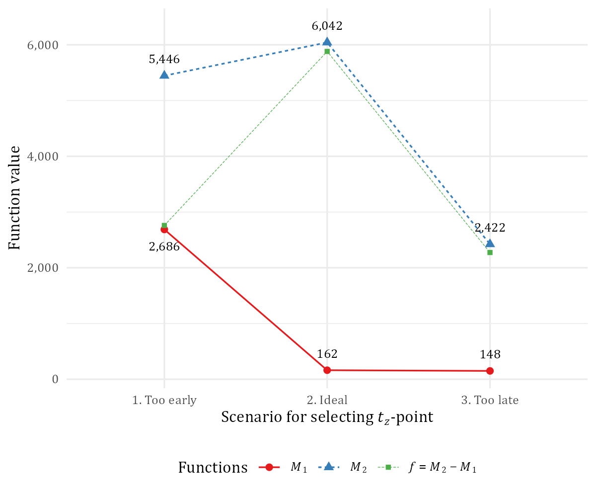
Figure 2: Illustrating three independent scenarios for $M_{1}$ and $M_{2}$ from Eqs. 4–5 in choosing the TZB-period’s starting point $t_{z}(i)$: too early, ideal, and too late. The function $f=M_{2}\big{(}t_{z}(i),\tau\big{)}-M_{1}\big{(}t_{z}(i)\big{)}$ illustrates the combined effect across all scenarios, shown in green.

Put differently, a delayed $t_{z}$-point will yield smaller $M_{2}(t_{z},\tau)$-values whereas a premature $t_{z}$-point will produce larger $M_{1}(t_{z})$-values. Both factors suggest that the ideal $t_{z}(i)$-point for a TZB-account $i$ can be found by maximising $M_{2}$ and minimising $M_{1}$ with respect to $t_{z}(i)$, which is itself controlled by varying $b$ in $T_{z}(\boldsymbol{B}_{i},b)$ from Eq. 2. Doing so implies maximising the loan-level objective function

$$l_{i}\big{(}t_{z}(i)\big{)}=w\cdot M_{2}\big{(}t_{z}(i),\tau\big{)}-M_{1}\big{(}t_{z}(i)\big{)}\quad\text{for}\ w\in[0,1]\quad\text{and}\quad\forall\ i\in\mathcal{S}_{T}\left(\boldsymbol{B},b\right)\,.$$ (7)

The specifiable weight $w$ in Eq. 7 is simply a mathematical expedient, which is motivated as follows. In isolating the TZB-account’s "true end", any reasonable $t_{z}(i)$-value also implies that the associated $M_{2}\big{(}t_{z}(i),\tau\big{)}$-value will most likely be orders of magnitude larger than its sibling $M_{1}\big{(}t_{z}(i)\big{)}$-value. In turn, this discrepancy in domain sizes imply that the value of $M_{2}$ will remain relatively unchanged when subtracting that of $M_{1}$, thereby rendering the latter as meaningless and ruining any subsequent optimisation. Accordingly, we introduce the specifiable weight $w$ in Eq. 7 by which $M_{2}$ should be scaled towards matching the domain of $M_{1}$, even if only approximately.

Finding a single portfolio-level threshold $b$ implies evaluating Eq. 7 across many TZB-accounts. For a particular $(\boldsymbol{B},b)$-tuple (or ‘configuration’), the final portfolio-level objective function therefore becomes

$$f(\boldsymbol{B},b)=\frac{1}{\bar{s}}\sum_{i}{l_{i}\big{(}T_{z}(\boldsymbol{B}_{i},b)\big{)}}\quad\text{for}\ \forall\ i\in\mathcal{S}_{T}(\boldsymbol{B},b)\,.$$ (8)

Since the size and composition of $\mathcal{S}_{T}(\boldsymbol{B},b)$ will change in tandem with each $(\boldsymbol{B},b)$-configuration, the eventual optimisation will undoubtedly be affected by sampling variability. In mitigating this effect, the summation in Eq. 8 is therefore weighted by the sample standard deviation $\bar{s}$ of the loan-level $l_{i}\big{(}T_{z}(\boldsymbol{B}_{i},b)\big{)}$-values within $\mathcal{S}_{T}(\boldsymbol{B},b)$, which is the so-called TZB-set. More formally, let $n_{s}$ denote the size (or cardinality) of $\mathcal{S}_{T}(\boldsymbol{B},b)$, whereafter we estimate the mean $\bar{l}$ of these $l_{i}\big{(}T_{z}(\boldsymbol{B}_{i},b)\big{)}$-values as

$$\bar{l}=\frac{1}{n_{s}}\sum_{i}{l_{i}\big{(}T_{z}(\boldsymbol{B}_{i},b)\big{)}}\quad\text{for}\ \forall\ i\in\mathcal{S}_{T}(\boldsymbol{B},b)\,.$$ (9)

Using $\bar{l}$, we then estimate the standard deviation $\bar{s}$ as

$$\bar{s}=\sqrt{\frac{1}{n_{s}-1}\sum_{i}{\bigg{(}l_{i}\big{(}T_{z}(\boldsymbol{B}_{i},b)\big{)}-\bar{l}\bigg{)}^{2}}}\quad\text{for}\ \forall\ i\in\mathcal{S}_{T}(\boldsymbol{B},b)\,.$$ (10)

Finally, the objective function $f$ from Eq. 8 is iteratively calculated across a range of candidate thresholds $b\in\mathcal{S}_{b}$ within the search space $\mathcal{S}_{b}$, having used $\boldsymbol{B}$ as a particular control variable. Similar to the LROD-procedure from [46] and [47], the optimisation problem is effectively partitioned into smaller $(\boldsymbol{B},b)$-based ‘sub-problems’, where $\boldsymbol{B}$ can be any quantity used as a control and screened using $b$ as a domain-specific threshold. Each resulting $f(\boldsymbol{B},b)$-value is stored centrally, thereby forming a curve across all pre-chosen $b$-values for each $\boldsymbol{B}$, as demonstrated hypothetically in Fig. 3. The objective is then solved by searching for the ‘best’ threshold $b^{*}$ such that $f(\boldsymbol{B},b^{*})\geq f(\boldsymbol{B},b)$ across all candidate $b$-values within the search space $\mathcal{S}_{b}$. This $b^{*}$-value is then used in finding the start times of TZB-periods $T_{z}(\boldsymbol{B}_{i},b^{*})$ of each applicable account $i$ within the underlying TZB-set $\mathcal{S}_{T}\left(\boldsymbol{B},b^{*}\right)$, whereafter all monthly records are discarded for those times $T_{z}(\boldsymbol{B}_{i},b^{*}),\dots,T_{i}$, given that these accounts actually ended at $T_{z}(\boldsymbol{B}_{i},b^{*})-1$. The TruEnd-procedure is therefore summarised into the following general steps:

1. Enumerate the search space $\mathcal{S}_{b}$ with thresholds $b_{1},b_{2},\dots$ respective to the domain of a control $\boldsymbol{B}$;

2. Calculate $f(\boldsymbol{B},b)$ for every $(\boldsymbol{B},b)$-configuration within $\mathcal{S}_{b}$, and collate into the collection $\big{\{}f(\boldsymbol{B},b)\big{\}}$;

3. Search the collection $\big{\{}f(\boldsymbol{B},b)\big{\}}$ for the global maximum, i.e., the optimal threshold $b^{*}$ is given for each $\boldsymbol{B}$ by

   $$b^{*}=\mathop{\arg\max}_{b\,\in\,\mathcal{S}_{b}}{\left\{f(\boldsymbol{B},b)\right\}}\,;$$ (11)

4. Discard all records across times $t=T_{z}(\boldsymbol{B}_{i},b^{*}),\dots,T_{i}$ for all applicable accounts $i\in\mathcal{S}_{T}\left(\boldsymbol{B},b^{*}\right)$.

Figure 3: Illustrating the TruEnd-procedure in finding the optimal threshold $b^{*}$ that maximises the objective function $f$ from Eq. 8. Given a control variable $\boldsymbol{B}$ (e.g., balance), the elements within this times series that are smaller than $b^{*}$ can then be discarded, moving backwards.

3   Illustrating the TruEnd-procedure using residential mortgage data

The TruEnd-procedure is illustrated and tested using a rich portfolio of residential mortgages, provided by a large South African bank. This longitudinal dataset has monthly loan performance observations over time $t=1,...,T_{i}$ for account $i=1,...,N$ with $N=653,331$ 20-year mortgage accounts. These amortising mortgages were observed from January 2007 up to December 2022, during which new mortgages were continuously originated, thereby yielding 49,880,588 raw monthly observations of loan repayment performance. This data includes net cash flows (receipts), expected instalments, arrears balances, month-end balances, variable interest rates, original loan principals, re-advance amounts and times, write-off amounts and times, and early settlement amounts and times. Having prepared and cleaned this data extensively, we present the optimisation results in subsection 3.1 across a few subsamples of this data on which the TruEnd-procedure is applied. Then, we select the optimal threshold from these results and perform an impact study in subsection 3.2, wherein the dataset is compared before and after excluding the TZB-periods, as isolated using this optimal threshold.

3.1.   Optimisation results using the datasets $\mathcal{D}_{s}$ and $\mathcal{D}_{f}$

In applying the TruEnd-procedure on a loan portfolio of size $N$, a value must first be assigned to the weight $w\in[0,1]$ in Eq. 7 for down-scaling the non-TZB mean $M_{2}$, lest the effect of the (much smaller) TZB-mean $M_{1}$ becomes negligible. Consider that the contamination degree $\phi$ from Eq. 6 already represents the percentage-valued contribution of $M_{1}$ to the sum $M_{1}+M_{2}$; an intuitive basis from which we can derive a $w$-value at the portfolio-level. For each candidate threshold $b$, we calculate the means of both $M_{1}$ and $M_{2}$ across all applicable accounts, denoted respectively as $\bar{M}_{1}$ and $\bar{M}_{2}$. More formally, the portfolio-level contamination degree $\bar{\phi}(\boldsymbol{B},b)$ is estimated for each $b\in\mathcal{S}_{b}$ respective to a given control $\boldsymbol{B}$ as

$$\bar{\phi}(\boldsymbol{B},b)=\frac{\bar{M}_{1}(\boldsymbol{B},b)}{\bar{M}_{1}(\boldsymbol{B},b)+\bar{M}_{2}(\boldsymbol{B},b)}\,,$$ (12)

where its components are simply estimated as

$$\bar{M}_{1}(\boldsymbol{B},b) =\frac{1}{n_{s}}\sum_{i\,\in\,\mathcal{S}_{T}(\boldsymbol{B},b)}{M_{1}\Big{(}T_{z}(\boldsymbol{B}_{i},b)\Big{)}}\,,\ \text{and}$$

$$\bar{M}_{2}(\boldsymbol{B},b) =\frac{1}{N}\left(\sum_{i\,\in\,\mathcal{S}_{T}(\boldsymbol{B},b)}{M_{2}\Big{(}T_{z}(\boldsymbol{B}_{i},b),\tau\Big{)}}+\sum_{j\,\notin\,\mathcal{S}_{T}(\boldsymbol{B},b)}{M_{2}\Big{(}T_{j},\tau\Big{)}}\right)\quad\text{for}\ \tau=6\ \text{months}\,.$$

Figure 4: Portfolio-level contamination degree $\bar{\phi}(\boldsymbol{B},b)$ from Eq. 12 across candidate thresholds $b$ respective to account balances $\boldsymbol{B}$ as control. The midpoint is overlaid, which informs the $w$-value within the TruEnd-procedure.

We graph the contamination degree $\bar{\phi}(\boldsymbol{B},b)$ in Fig. 4 across several candidate thresholds $b\in\mathcal{S}_{b}$, where the search space is enumerated using expert judgement as

$$\mathcal{S}_{b}=\{ 0;10;25;50;75;100;150;200;250;300;400;500;750;1,000;1,250;$$

$$1,500;1,750;2,000;2,500;3,000;4,000;5,000;7,500;10,000\}\,.$$ (13)

Evidently, the $\bar{\phi}(\boldsymbol{B},b)$-quantity appears to be a monotonically increasing function of $b$, and even somewhat linear. This result is intuitively sensible since $\bar{M}_{1}(\boldsymbol{B},b)$ should increase in tandem with $b$, especially when denoting balances smaller than $b$ as "practically zero-valued" towards identifying TZB-periods later. Then, we define the so-called midpoint across all contamination degrees as the average $\bar{\phi}(\boldsymbol{B},b)$-value between the lowest and highest of such degrees; i.e., $50\%\cdot\sum{\bar{\phi}(\boldsymbol{B},b)}$ for the first and last $b$-values within $\mathcal{S}_{b}$ from subsection 3.1. The resulting midpoint of 0.065% is then used as the $w$-value in Eq. 7, thereby calibrating the TruEnd-procedure towards this particular mortgage portfolio. This rather simplistic method for finding a $w$-value produces reasonable and intuitive optimisation results, as will be shown later. However, future research can most certainly improve upon this aspect of calibrating the TruEnd-procedure, as well as examine the impact of the chosen $\tau$-value.

Given the extremely large sample sizes, we deliberately subsample the full dataset $\mathcal{D}_{f}$ into a smaller set $\mathcal{D}_{s}$ using clustered random sampling. This $\mathcal{D}_{s}$-set contains the entire repayment histories of only 10,000 mortgage accounts that were randomly selected, which effectively constitutes only 1.5% of all accounts within $\mathcal{D}_{f}$. The TruEnd-procedure can then be applied on both of these sets $\left\{\mathcal{D}_{f};\mathcal{D}_{s}\right\}$, whereupon the resulting optima can be compared with respect to the influence of sample size. Such an analysis can help inspire confidence in the overall robustness of optima, or highlight instability related to overly small sample sizes. As a first step, we repeat the analysis shown in Fig. 4 by using the smaller $\mathcal{D}_{s}$ with Eq. 12 in estimating the portfolio contamination degrees $\bar{\phi}(\boldsymbol{B},b)$. The resulting differences in the $\bar{\phi}(\boldsymbol{B},b)$-values are almost indiscernible across all $b$-thresholds when using $\mathcal{D}_{s}$ instead of $\mathcal{D}_{f}$. That said, the midpoint changed every so slightly from 0.065% ($\mathcal{D}_{f}$) to 0.064% ($\mathcal{D}_{s}$). These minute differences in $\bar{\phi}(\boldsymbol{B},b)$-values already suggest some robustness against ‘small’ sample sizes; however, this result is highly dependent on the exact size of $\mathcal{D}_{s}$ and random sampling.

We present the so-called TruEnd-results in Fig. 5 across the same search space $b\in\mathcal{S}_{b}$ from subsection 3.1 and for the same control variable $\boldsymbol{B}$ (balances), having iteratively estimated $f(\boldsymbol{B},b)$ from Eq. 8 on both of the datasets $\left\{\mathcal{D}_{s},\mathcal{D}_{f}\right\}$. The results are strikingly similar in that both datasets produce an $f$-curve with the same shape, as well as yield the same optimal $b^{*}$-value of ZAR 300 that can serve as a "small-balance definition" (or policy). The optimal region that contains this $b^{*}$-value is slightly larger for the smaller set $\mathcal{D}_{s}$ than for $\mathcal{D}_{f}$, though this discrepancy is attributable to sampling variability; itself corroborated when comparing the slightly perturbed shape of the $f$-curve in Fig. 5(a) to the smoother shape in Fig. 5(b). Moreover, the $b$-values within this optimal region, i.e., $b\in[200,500]$, do not differ significantly from one another on their face value; as corroborated by the relatively small differences in their $f(\boldsymbol{B},b)$-values. By implication, any of these $b$-values can serve quite intuitively as small-balance definitions in practice, despite $b^{*}$ being the ‘best’ such value. Conversely, more extreme $b$-values such as $b<100$ or $b\geq 2,500$ are correctly disqualified in Fig. 5 given their increasing sub-optimality. These results therefore provide high-level assurance on the soundness and robustness of the TruEnd-procedure and its optima.

(a) TruEnd-results on the subsampled set $\mathcal{D}_{s}$

(b) TruEnd-results on the full set $\mathcal{D}_{f}$

Figure 5: TruEnd-results $f\left(\boldsymbol{B},b\right)$ across candidate thresholds $b$, respective to account balances $\boldsymbol{B}$ as control. The encircled point denotes the best policy $b^{*}$ that maximises $f$ from Eq. 8. The pink triangular points that surround $b^{*}$ signify an optimal region in $f$ as annotated. The TruEnd-results are respectively derived in (a) and (b) from either the smaller subsampled dataset $\mathcal{D}_{s}$ or from the full dataset $\mathcal{D}_{f}$.

In principle, the prevalence of any phenomenon depends on the definition thereof. Likewise, the portfolio-wide prevalence of accounts with a TZB-period will also depend on the exact definition of a "small balance" used in isolating such TZB-periods, i.e., the candidate $b$-values. Given a particular $b$-value, recall the decision function $Z_{it}(B_{it},b)$ from Eq. 3 that indicates at time $t$ whether account $i$ is in its TZB-period or not; i.e., the respective value 1 or 0. We aggregate these values for each $i$ by taking the maximum over $t$, whereafter these aggregates are denoted as $Z_{i}(\boldsymbol{B}_{i},b)$ given each balance vector $\boldsymbol{B}_{i}$. These account-level TZB-indicators form a sample of size $N$ from which the so-called TZB-prevalence rate can be estimated at the portfolio-level. Expressed as $\sum_{i}{Z_{i}(\boldsymbol{B}_{i},b)/N}$, we graph the resulting TZB-prevalence rate in Fig. 6 across the same $b$-values using $\mathcal{D}_{f}$. Evidently, TZB-prevalence increases rapidly as $b$ increases, though its slope flattens progressively for points beyond the optimal $b^{*}$-policy. With a range of approximately 15-28%, overall TZB-prevalence is remarkably sensitive to the choice of $b$, especially when considering that TZB-prevalence almost doubles when comparing the extremities. The optimal $b^{*}$-policy itself yields a TZB-prevalence rate of 23% for $\mathcal{D}_{f}$, which remains practically unchanged at 22.7% for the smaller dataset $\mathcal{D}_{s}$. Almost a quarter of the portfolio’s accounts are therefore afflicted with this pernicious TZB-error, which would have likely remained undetected if not for applying the TruEnd-procedure.

Figure 6: The TZB-prevalence rate across candidate thresholds $b$, respective to account balances $\boldsymbol{B}$ as control within the full dataset $\mathcal{D}_{f}$. Given the optimal $b^{*}$-policy from Fig. 5, the associated TZB-prevalence rate is overlaid.

The high TZB-prevalence rates presented thus far are certainly worrisome, given the potential for severely biased predictions from subsequent time-to-event models. However, the degree of such bias will inherently depend on the materiality (or impact) of TZB-cases, even if quite prevalent within a portfolio. For each candidate threshold $b$ in Fig. 7, we therefore investigate the impact of imposing such a $b$-policy, having discarded the resulting TZB-period for each affected account. Starting at 98.7 months for $b=0$, the mean account age in Fig. 7(a) decreases swiftly at first as $b$ increases up to the optimal $b^{*}$-policy, at which point the loans have a shorter average lifetime of 96.7 months. The mean length of these discarded TZB-periods also increases as $b$ grows slightly larger; i.e., from 13.9 to 18.5 months for $b=0,\dots,b^{*}$. The respective downward and upward trends in both means are intrinsically sensible since we fully expect the mean age to decrease when discarding TZB-periods of greater length as $b$ increases. However, for larger $b$-values, the rate of change in both of these means slows down noticeably after reaching the optimal $b^{*}$-policy, despite the increments between successive $b$-values growing larger. These flatter slopes suggest that the TruEnd-procedure has greater impact for smaller $b$-values given the greater sensitivity to changes at those smaller locales. Moreover, the mean loan age of 100.9 months within the raw dataset decreases quite significantly by about 4.2 months when imposing the optimal $b^{*}$-policy and discarding the resulting TZB-periods; themselves having a mean length of 18.5 months and median of 5 months. Accordingly, certain risk events such as write-off or early settlement can occur far earlier than previously thought, which has sobering implications for the degree of ‘mistimed’ predictions from survival models.

(a) Mean account ages

(b) Mean balances

Figure 7: Sample mean values of various measures across candidate thresholds $b$, respective to account balances $\boldsymbol{B}$ as control within the full dataset $\mathcal{D}_{f}$. Error margins (shaded) are overlaid for each estimate using 95% confidence intervals; some of which are very narrow and barely visible. Given the optimal $b^{*}$-policy from Fig. 5, the associated means are annotated. In (a), the means of account ages and TZB-period lengths are shown in the respective sub-panels. In (b), the portfolio-level means $\bar{M}_{1}(\boldsymbol{B},b)$ and $\bar{M}_{2}(\boldsymbol{B},b)$ from Eq. 12 are shown in the respective sub-panels.

Aside from analysing the age-related impact of applying the TZB-procedure, we also examine its impact in Fig. 7(b) from the perspective of monetary value. In particular, the portfolio-level mean $\bar{M}_{1}$ appears to be a monotonically increasing function of the candidate threshold $b$, which is unsurprising given the role of $b$ in qualifying balances as TZB-cases. Moreover, the mean balances during these TZB-periods are reassuringly small across most $b$-values, at least up to the optimal $b^{*}$-policy; at which point the mean is approximately ZAR 7.45. This empirical result corroborates the intuition that a TZB-period should – by definition – only span those last few balances that are "practically zero-valued". The monetary impact on the portfolio would therefore be minuscule when discarding these isolated TZB-periods, especially for smaller $b$-values. Furthermore, the other portfolio-level mean $M_{2}$ also seems to be a monotonically increasing function of $b$. Such an increasing trend is innately sensible since small-valued outlying TZB-cases are increasingly removed from the window over which $\bar{M}_{2}$ is calculated, thereby ‘sifting’ the mean. However, and unlike $\bar{M}_{1}$, the rate of change in $\bar{M}_{2}$ is far greater for smaller values of $b\leq b^{*}$ than for larger values; just like for the means of loan age and TZB-period length in Fig. 7(a). Lastly, all of these results in Fig. 7 do not change materially when using the smaller dataset $\mathcal{D}_{s}$ instead of $\mathcal{D}_{f}$, thereby providing at least some assurance on their robustness against sampling variability. Assuming the optimal $b^{*}$-policy, we therefore conclude that TZB-cases are not only quite prevalent in affecting 23% of accounts, but can materially prejudice the timing of risk events given the surprisingly long trail of excessive history ($\geq 18$ months). Excluding these trails will correct the timing though without affecting the overall portfolio size, given the very low mean TZB-balance of $\bar{M}_{1}(\boldsymbol{B},b^{*})=$ ZAR 7.45.

3.2.   The impact of applying the TruEnd-procedure vs its absence

Following subsection 3.1, we duly select the optimal policy $b^{*}=300$ in serving as the portfolio-wide cut-off for identifying the start times of TZB-periods; i.e., $b^{*}$ is the ‘best’ small-balance definition. However, this $b^{*}$-policy is selectively applied in that the resulting TZB-periods are discarded only for terminated accounts, i.e., write-offs and settlements. Doing so is deemed prudent in limiting the potential for unwittingly ‘overwriting’ the observed reality (or data) when discarding records, at least beyond what is necessary. Furthermore, it so happens that these terminated accounts constitute 83% of identified TZB-cases, while the remaining minority cases are still active (or right-censored) by the end of the sampling window. This rather high prevalence of terminated accounts within TZB-cases actually corroborates the original description of the problem; i.e., operational and/or system failures can delay the timely closure of accounts, thereby corrupting their observed endpoints.

(a) Overall account lifetimes

(b) Realised loss rates (write-offs)

Figure 8: A distributional analysis in comparing the histograms and densities of certain quantities in the full dataset $\mathcal{D}_{f}$, before and after discarding the isolated TZB-cases using the optimal $b^{*}$-policy. Sample means are overlaid, showing a 3-month reduction in the average account age in (a); and a 1.2% point reduction in the average realised loss in (b).

Having excluded the identified TZB-periods using this $b^{*}$-policy, we examine the impact thereof using a comparative distributional analysis. In particular, the empirical probability distribution of a certain quantity is analysed against that of its ‘predecessor’; i.e., the true distribution $f_{\mathrm{T}}$ that rightfully excludes TZB-periods vs the preceding false distribution $f_{\mathrm{F}}$ that still includes TZB-periods. By virtue of shortening some account histories, we fully expect account ages $a$ to be affected, which should reflect in the distributional shapes of $f_{\mathrm{F}}$ and $f_{\mathrm{T}}$ across $a$. In fact, Fig. 8(a) shows that $f_{\mathrm{F}}(a)<f_{\mathrm{T}}(a)$ for smaller ages $a<80$ months, which reverses to $f_{\mathrm{F}}(a)>f_{\mathrm{T}}(a)$ for larger ages $a>240$; a clockwise "distributional tilt" in the shape of $f_{\mathrm{T}}$ relative to that of $f_{\mathrm{F}}$. The overall mean age reduces by 3 months to 97.9 when applying this $b^{*}$-policy, even though its effect is much more pronounced for terminated accounts – in which case, the mean age reduces by about 18 months. Moreover, we obtain a similar result for the realised loss rates $l$, as calculated from written-off accounts using the workout-method with observed cash flows; see [55] and [39, §10 ]. Specifically, $f_{\mathrm{T}}$ also exhibits a clockwise distributional tilt relative to $f_{\mathrm{F}}$ across all $l$, as shown in Fig. 8(b). The mean loss rate therefore decreases by 1.2% points to 40.5% when applying this $b^{*}$-policy. While seemingly small, this reduction can amount to many millions saved in credit losses for typical mortgage portfolios, purely as an innocuous data fix before any intensive modelling.

One can also gauge the impact of imposing this $b^{*}$-policy by using survival analysis to model another aspect of the LGD risk parameter: the time until write-off $T$. This non-negative random variable $T$ represents the age of a default spell that either ends with a resolved outcome (write-off) or is left unresolved as right-censored. Then, consider the cumulative lifetime probability distribution $F(t)=\mathbb{P}(T\leq t)$ across some time horizon $t$, which represents the cumulative probability of write-off by time $t$; see [61, pp. 1-15 ]. Its complement is the write-off survivor function $S(t)=1-F(t)=\mathbb{P}(T>t)$, which may be estimated using the well-known non-parametric Kaplan-Meier (KM) estimator $\hat{S}(t)$ from [59]. Regarding competing risks that preclude write-off, the cured outcome is grouped with right-censored observations in the interest of expediency and simplicity. However, by following this "latent risks" approach, the quantity $\hat{F}(t)=1-\hat{S}(t)$ can be overestimated, as discussed in [54]. That said, the effects of such overestimation should at least be consistent within a broader two-component comparative study, especially when both components $A$ and $B$ are equally overestimated in assessing the difference $A-B$; itself the main objective at present. We therefore deem such overestimation to be negligible in its effect on the ensuing comparative study.

We present the $\hat{F}(t)$-estimates in Fig. 9 and compare the true distribution $F_{\mathrm{T}}(t)$ that rightfully excludes TZB-periods vs the false distribution $F_{\mathrm{F}}(t)$ that still includes TZB-periods; i.e., applying the TruEnd-procedure vs its absence. The difference between both cumulative distributions seems to grow up to a certain time point $t=84$, beyond which the difference gradually subsides again. The slightly larger lifetime write-off probabilities $F_{\mathrm{T}}(t)>F_{\mathrm{F}}(t)$ stem directly from the act of excluding TZB-periods, thereby moving risk events to earlier times during default spells. This result is corroborated in Fig. 10 wherein we provide estimates of the discrete-time hazard rate $\hat{h}(t)=\hat{f}(t)/\hat{S}(t)$, where $\hat{f}$ is the estimated density function of $\hat{F}$ that represents the frequency of failures per unit of time. The write-off hazard $\hat{h}(t)$ therefore denotes the conditional write-off probability of an account during $(t-1,t]$, having survived at least up to $t-1$. Accordingly, estimates of the true hazard distribution $h_{\mathrm{T}}(t)$ that rightfully exclude TZB-periods are compared to those of the false hazard distribution $h_{\mathrm{F}}(t)$ that still include TZB-periods. Again, we observe slightly larger write-off hazards $h_{\mathrm{T}}(t)\geq h_{\mathrm{F}}(t)$ at earlier times $t\leq 84$, though these differences grow smaller (and even reverse) at later times. While write-off risk evidently increases when correcting the timing of the underlying risk events, the realised loss rates can decrease by virtue of shorter default spells, as previously shown in Fig. 8. Lastly, default spells longer than 10 years are increasingly rare and of dubious practical value. We have therefore limited the (graphical) survival analyses of both $\hat{F}(t)$ and $\hat{h}(t)$ in Figs. 9–10 to a maximum time in default of 10 years, without necessarily excluding those longer-aged default spells.

(a) Early time period $t\in[0,60]$

(b) Later time period $t\in[61,120]$

Figure 9: Comparing the cumulative lifetime probability distribution $\hat{F}(t)$ over spell age $t$ until write-off, having applied the TruEnd-procedure ($F_{\mathrm{T}}$) vs its absence ($F_{\mathrm{F}}$). In (a), $F(t)$ is graphed for the early period $t\in[0,60]$, whereas (b) shows the later period $\in[61,120]$. In summarising the discrepancy between the line graphs $A_{t}$ and $B_{t}$, the mean absolute error (MAE) is calculated and overlaid.

(a) Early time period $t\in[0,60]$

(b) Later time period $t\in[61,120]$

Figure 10: Comparing the hazard function $\hat{h}(t)$ over spell age $t$ until write-off, having applied the TruEnd-procedure ($h_{\mathrm{T}}$) vs its absence ($h_{\mathrm{F}}$); shown across two periods in (a) and (b). The graph design follows that of Fig. 9.

4   Conclusion

In credit data, an account’s observed repayment history can incorrectly include a lengthy sequence of zero (or very small) month-end balances towards its end, often caused by operational or system failures that delay the account’s timely closure. This phenomenon, called trailing zero-valued balances (TZB), poses a significant modelling challenge since it distorts the ‘true’ but unobservable endpoints of affected accounts. As a form of measurement error, these TZB-cases can ruin the timing of certain risk events such as write-off or early settlement. When training LGD-models from affected data, TZB-cases become particularly pernicious to the resulting loss predictions. The excess TZB-history can artificially prolong the period over which cash flows are discounted, thereby inflating the calculated loss percentage even before modelling such ‘realised’ losses. Moreover, inaccurate timings of risk events in training data can compromise the subsequent predictions of any time-to-event model, including survival analysis. Therefore, the failure to identify and treat these TZB-cases will invite model risk, which can erode trust in all statistical models derived from such inaccurate data.

The remedy is intuitively simple: remove the ‘cancerous’ TZB-affected part within the history of a loan, thereby moving its endpoint earlier. However, finding the ‘true’ endpoint for each loan is difficult at scale, especially given the typically large sizes of credit datasets in retail lending. An automated procedure of sorts is clearly needed, though which would then need instruction on identifying these TZB-cases; itself a non-trivial task. Isolating such trails of diminutive balances will depend on the exact definition of a "small or immaterial" balance, which should itself be neither too small nor too large, lest we either retain false history or discard credible history. Determining the ‘best’ definition $b^{*}$ amidst many candidates $b$ would require an optimisation approach that embeds the underlying costs/benefits of each $b$-value. Such an approach would also need to contend with the uncertainty of account balances over time; i.e., the potential for settlement and bouts of loan delinquency, which may even end in write-off. Moreover, the approach would need to find a single small-balance definition that can apply to the entire portfolio (or homogeneous segment therein), thereby exerting appropriate control while achieving consistency and simplicity.

We contribute such a data-driven optimisation approach that can find the best small-balance policy $b^{*}$ towards identifying and discarding latent TZB-periods within a given loan portfolio. Our so-called TruEnd-procedure includes a bespoke objective function $f$ that is statistically evaluated across the histories of all constituent accounts. This $f$ relies on two opposing counter-measures, $M_{2}$ and $M_{1}$; both of which giving the mean balance of an account, albeit calculated over two different periods that respectively predate or succeed the supposed ‘true’ endpoint. When optimising $f$ using a value iteration technique, the best $b^{*}$-policy effectively yields those individual endpoints within affected loan histories that simultaneously maximises $M_{2}$ and minimises $M_{1}$ on average. Some of the novelty in these measures arises from their deliberate exploitation of the arithmetic mean’s known weakness to outliers. Having identified the true endpoints using this $b^{*}$-policy, the excess histories thereafter constitute TZB-periods that can be discarded, thereby correcting the timing of account termination.

In demonstrating the TruEnd-procedure, we test a wide range of candidate policies $b$ in defining "small balances", having used a large sample of residential mortgage data from the South African credit market. Not only do we find the best $b^{*}$-policy, but our results also reveal a small optimal region of $b$-values clustered around this $b^{*}$-value. The optimisation results $f(b)$ are strikingly similar for those $b$-values within this region, which suggests that any one of them can practically serve as a policy definition for "small balances". However, the function $f$ reacts ever more drastically to larger values of $b$ outside of this region, whilst noting that such larger $b$-values would increasingly curtail the individual loan histories to their detriment. As $b$ grows larger beyond a certain point, the notion of cutting away more and more of the ‘healthy’ parts of these histories should rightfully be penalised accordingly. Therefore, the associated and demonstrably severe reaction in $f$ serves as reassurance on the overall and intuitive soundness of the TruEnd-procedure in definitively disqualifying those larger $b$-values.

Aside from finding the optimal $b^{*}$-policy, TZB-affected accounts are remarkably prevalent within this mortgage portfolio, ranging at 15-28% of accounts across all $b$-values. When applying any of these $b$-policies, the isolated (and discarded) TZB-periods have significant durations in that loan histories are now shortened by about 14-19 months on average, depending on the exact $b$-value. Evidently, TZB-cases are both highly prevalent and material in this portfolio, which could not have been detected (or even quantified) if not for applying our TruEnd-procedure. At the optimal $b^{*}$-policy of ZAR 300, we find that 23% of accounts are TZB-cases with excess histories that span about 18 months, during which time the mean TZB-balance is practically zero-valued at ZAR 7.45. Having discarded the identified TZB-periods, the timing of account termination is therefore corrected, thereby reducing the mean loss rate of write-offs by 1.2% points; a material result for any LGD-model. Using survival analysis on defaulted loans, we further interrogate this result by modelling and comparing the now-corrected time to write-off versus its uncorrected counterpart. As expected, the write-off hazard generally increases at earlier durations within default spells, chiefly due to risk events now occurring slightly earlier than before. Both the predicted timing and severity of risk events are therefore made more accurate in modelling the recovery process of defaulted loans. By implication, the resulting LGD-model yields lower and less-biased estimates of credit losses for defaulted loans, having better approximated their true profiles of credit risk. Ultimately, we believe this work can safely salvage a dataset that is otherwise corrupted by TZB-cases, which demonstrates the sound pursuit of innovation during data preparation.

Regarding limitations, the TruEnd-procedure currently uses monthly account balances $\boldsymbol{B}$ as the control variable in screening candidate thresholds $b$, respective to the domain of $\boldsymbol{B}$. However, these currency-denominated amounts are certainly susceptible to the erosive effects of inflation, especially over longer sampling periods. This inflation susceptibility can detract from finding a single ideal threshold $b^{*}$ that should apply to all balances across time. Future research can therefore explore alternative controls such as the balance-to-principal ratio of an account over time, whose percentage-valued bounds can circumvent the aforementioned inflation susceptibility. In addition, future researchers can refactor the TruEnd-procedure towards using multiple control variables, e.g., both balance and balance-to-principal. Using multiple controls may afford even greater granularity in the search for optimal thresholds, though the added complexity thereof may become questionable. Similarly, one could also explore the value of a segmentation scheme by which the underlying dataset is first partitioned before running the optimisation step. Instead of yielding a single portfolio-wide threshold $b^{*}$, such future work can focus on finding an optimised threshold $b^{*}_{s}$ for each homogeneous segment $s$ of accounts.

Acknowledgements

This study is partially supported by the National Research Foundation of South Africa (Grant Number 126885). This work has no known conflicts of interest that may have influenced the outcome of this work. The authors also thank all anonymous referees and editors for their valuable contributions.

References

- [1] Bart Baesens, Daniel Rösch and Harald Scheule “Credit Risk Analytics: Measurement Techniques, Applications, and Examples in SAS” Hoboken, New Jersey: John Wiley & Sons, 2016
- [2] John Banasik, Jonathan N Crook and Lyn C Thomas “Not if but when will borrowers default” In Journal of the Operational Research Society 50.12 JSTOR, 1999, pp. 1185–1190 DOI: 10.1057/palgrave.jors.2600851
- [3] Tony Bellotti and Jonathan Crook “Credit scoring with macroeconomic variables using survival analysis” In Journal of the Operational Research Society 60.12 Nature Publishing Group, 2009, pp. 1699–1707 DOI: 10.1057/jors.2008.130
- [4] Tony Bellotti and Jonathan Crook “Forecasting and stress testing credit card default using dynamic models” In International Journal of Forecasting 29.4, 2013, pp. 563–574 DOI: 10.1016/j.ijforecast.2013.04.003
-
[5]
Tony Bellotti and Jonathan Crook
“Retail credit stress testing using a discrete hazard model with macroeconomic factors”
In Journal of the Operational Research Society 65.3
Taylor
& Francis, 2014, pp. 340–350 DOI: 10.1057/jors.2013.91 - [6] Arno Botha “A procedure for loss-optimising the timing of loan recovery under uncertainty”, 2021 DOI: 10.13140/RG.2.2.12015.30888/1
- [7] Arno Botha and Roelinde Bester “The TruEnd-procedure [source code] for treating trailing zero-valued balances in credit data” Zenodo, 2024 DOI: 10.5281/zenodo.10974650
- [8] Arno Botha, Conrad Beyers and Pieter De Villiers “Simulation-based optimisation of the timing of loan recovery across different portfolios” In Expert Systems with Applications 177, 2021 DOI: 10.1016/j.eswa.2021.114878
- [9] Arno Botha, Conrad Beyers and Pieter De Villiers “The loss optimisation of loan recovery decision times using forecast cash flows” In Journal of Credit Risk, 2022 DOI: 10.21314/JCR.2020.275
- [10] Stephen Boyd and Lieven Vandenberghe “Convex optimization” Cambridge University Press, 2004
- [11] Raffaella Calabrese and Michele Zenga “Bank loan recovery rates: Measuring and nonparametric density estimation” In Journal of Banking & Finance 34.5 Elsevier, 2010, pp. 903–911 DOI: 10.1016/j.jbankfin.2009.10.001
- [12] Jonathan Crook and Tony Bellotti “Time Varying and dynamic models for default risk in consumer loans” In Journal of the Royal Statistical Society: Series A (Statistics in Society) 173.2, 2010, pp. 283–305 DOI: 10.1111/j.1467-985x.2009.00617.x
- [13] Pieter J. De Jongh et al. “A proposed best practice model validation framework for Banks” In South African Journal of Economic and Management Sciences 20.1, 2017 DOI: 10.4102/sajems.v20i1.1490
-
[14]
Lore Dirick, Gerda Claeskens and Bart Baesens
“Time to default in credit scoring using survival analysis: a benchmark study”
In Journal of the Operational Research Society 68.6
Taylor
& Francis, 2017, pp. 652–665 DOI: 10.1057/s41274-016-0128-9; - [15] Steven Finlay “The Management of Consumer Credit: Theory and Practice” Hampshire, UK: Palgrave Macmillan, 2010
- [16] Ted A Gooley, Wendy Leisenring, John Crowley and Barry E Storer “Estimation of failure probabilities in the presence of competing risks: new representations of old estimators” In Statistics in medicine 18.6 Wiley Online Library, 1999, pp. 695–706 DOI: 10.1002/(sici)1097-0258(19990330)18:6<695::aid-sim60>3.0.co;2-o
- [17] Marc Gürtler and Martin Hibbeln “Improvements in loss given default forecasts for bank loans” In Journal of Banking & Finance 37.7 Elsevier, 2013, pp. 2354–2366 DOI: 10.1016/j.jbankfin.2013.01.031
- [18] IASB “International Financial Reporting Standard (IFRS) 9: Financial Instruments”, 2014 IFRS Foundation: International Accounting Standards Board (IASB) URL: https://www.ifrs.org/issued-standards/list-of-standards/ifrs-9-financial-instruments/
- [19] Gareth James, Daniela Witten, Trevor Hastie and Robert Tibshirani “An introduction to statistical learning: with applications in R” New York: Springer, 2013 DOI: 10.1007/978-1-4614-7138-7
- [20] Morne Joubert, Tanja Verster and Helgard Raubenheimer “Making use of survival analysis to indirectly model loss given default” In ORiON 34.2 ORSSA, 2018, pp. 107–132 DOI: 10.5784/34-2-588
- [21] E.. Kaplan and Paul Meier “Nonparametric Estimation from Incomplete Observations” In Journal of the American Statistical Association 53.282 [American Statistical Association, Taylor & Francis, Ltd.], 1958, pp. 457–481 URL: http://www.jstor.org/stable/2281868
- [22] Christiana Kartsonaki “Survival analysis” In Diagnostic Histopathology 22.7 Elsevier, 2016, pp. 263–270 DOI: 10.1016/j.mpdhp.2016.06.005
- [23] David G Kleinbaum and Mitchel Klein “Survival analysis: a self-learning text” New York: Springer, 2012 DOI: 10.1007/978-1-4419-6646-9
- [24] Janette Larney, James Samuel Allison, Gerrit Lodewicus Grobler and Marius Smuts “Modelling the Time to Write-Off of Non-Performing Loans Using a Promotion Time Cure Model with Parametric Frailty” In Mathematics 11.10 MDPI, 2023, pp. 2228 DOI: 10.3390/math11102228
- [25] B Narain “Survival analysis and the credit granting decision” In Credit Scoring and Credit Control OUP, Oxford, UK, 1992, pp. 109–121
- [26] Zoltán Novotny-Farkas “The interaction of the IFRS 9 expected loss approach with supervisory rules and implications for financial stability” In Accounting in Europe 13.2, 2016, pp. 197–227 DOI: 10.1080/17449480.2016.1210180
- [27] PRA “PS6/23: Model risk management principles for banks”, 2023 Bank of England, Prudential Regulation Authority (PRA) URL: https://www.bankofengland.co.uk/prudential-regulation/publication/2023/may/model-risk-management-principles-for-banks
- [28] PRA “SS1/23: Model risk management principles for banks”, 2023 Bank of England, Prudential Regulation Authority (PRA) URL: https://www.bankofengland.co.uk/prudential-regulation/publication/2023/may/model-risk-management-principles-for-banks-ss
- [29] SARB “G9/2022: Matters related to the credit risk models of banks”, 2022 South African Reserve Bank (SARB): URL: https://www.resbank.co.za/en/home/publications/publication-detail-pages/prudential-authority/pa-deposit-takers/banks-guidance-notes/2022/G9-2022-Matters-related-to-the-credit-risk-models-of-banks
- [30] Patrick Schober and Thomas R Vetter “Survival analysis and interpretation of time-to-event data: the tortoise and the hare” In Anesthesia and Analgesia 127.3 Wolters Kluwer Health, 2018, pp. 792–798 DOI: 10.1213/ANE.0000000000003653
- [31] Til Schuermann “What do we know about Loss Given Default?” In Wharton Financial Institutions Centre Working Paper, Availaible at SSRN:, 2004 DOI: 10.2139/ssrn.525702
- [32] Judith D Singer and John B Willett “It’s about time: Using discrete-time survival analysis to study duration and the timing of events” In Journal of Educational Statistics 18.2, 1993, pp. 155–195 DOI: 10.2307/1165085
- [33] Jimmy Skoglund “Credit risk term-structures for Lifetime Impairment Forecasting: A practical guide” In Journal of Risk Management in Financial Institutions 10.2, 2017, pp. 177–195 URL: https://www.econbiz.de/Record/credit-risk-term-structures-for-lifetime-impairment-forecasting-a-practical-guide-skoglund-jimmy/10011670671
- [34] Maria Stepanova and Lyn Thomas “Survival analysis methods for personal loan data” In Operations Research 50.2 INFORMS, 2002, pp. 277–289 DOI: 10.1287/opre.50.2.277.426
- [35] Lyn C Thomas “Consumer Credit Models: Pricing, Profit and Portfolios” New York: Oxford University Press, 2009 DOI: 10.1093/acprof:oso/9780199232130.001.1
- [36] Jiri Witzany, Michal Rychnovsky and Pavel Charamza “Survival analysis in LGD modeling” In European Financial and Accounting Journal 7.1, 2012, pp. 6–27 DOI: 10.18267/j.efaj.12
- [37] Richard Wood and David Powell “Addressing probationary period within a competing risks survival model for retail mortgage loss given default” In Journal of Credit Risk 13.3, 2017 DOI: 10.21314/JCR.2017.228
- [38] Jie Zhang and Lyn C Thomas “Comparisons of linear regression and survival analysis using single and mixture distributions approaches in modelling LGD” In International Journal of Forecasting 28.1 Elsevier, 2012, pp. 204–215 DOI: 10.1016/j.ijforecast.2010.06.002
- [39] Bart Baesens, Daniel Rösch and Harald Scheule “Credit Risk Analytics: Measurement Techniques, Applications, and Examples in SAS” Hoboken, New Jersey: John Wiley & Sons, 2016
- [40] John Banasik, Jonathan N Crook and Lyn C Thomas “Not if but when will borrowers default” In Journal of the Operational Research Society 50.12 JSTOR, 1999, pp. 1185–1190 DOI: 10.1057/palgrave.jors.2600851
- [41] Tony Bellotti and Jonathan Crook “Credit scoring with macroeconomic variables using survival analysis” In Journal of the Operational Research Society 60.12 Nature Publishing Group, 2009, pp. 1699–1707 DOI: 10.1057/jors.2008.130
- [42] Tony Bellotti and Jonathan Crook “Forecasting and stress testing credit card default using dynamic models” In International Journal of Forecasting 29.4, 2013, pp. 563–574 DOI: 10.1016/j.ijforecast.2013.04.003
-
[43]
Tony Bellotti and Jonathan Crook
“Retail credit stress testing using a discrete hazard model with macroeconomic factors”
In Journal of the Operational Research Society 65.3
Taylor
& Francis, 2014, pp. 340–350 DOI: 10.1057/jors.2013.91 - [44] Arno Botha “A procedure for loss-optimising the timing of loan recovery under uncertainty”, 2021 DOI: 10.13140/RG.2.2.12015.30888/1
- [45] Arno Botha and Roelinde Bester “The TruEnd-procedure [source code] for treating trailing zero-valued balances in credit data” Zenodo, 2024 DOI: 10.5281/zenodo.10974650
- [46] Arno Botha, Conrad Beyers and Pieter De Villiers “Simulation-based optimisation of the timing of loan recovery across different portfolios” In Expert Systems with Applications 177, 2021 DOI: 10.1016/j.eswa.2021.114878
- [47] Arno Botha, Conrad Beyers and Pieter De Villiers “The loss optimisation of loan recovery decision times using forecast cash flows” In Journal of Credit Risk, 2022 DOI: 10.21314/JCR.2020.275
- [48] Stephen Boyd and Lieven Vandenberghe “Convex optimization” Cambridge University Press, 2004
- [49] Raffaella Calabrese and Michele Zenga “Bank loan recovery rates: Measuring and nonparametric density estimation” In Journal of Banking & Finance 34.5 Elsevier, 2010, pp. 903–911 DOI: 10.1016/j.jbankfin.2009.10.001
- [50] Jonathan Crook and Tony Bellotti “Time Varying and dynamic models for default risk in consumer loans” In Journal of the Royal Statistical Society: Series A (Statistics in Society) 173.2, 2010, pp. 283–305 DOI: 10.1111/j.1467-985x.2009.00617.x
- [51] Pieter J. De Jongh et al. “A proposed best practice model validation framework for Banks” In South African Journal of Economic and Management Sciences 20.1, 2017 DOI: 10.4102/sajems.v20i1.1490
-
[52]
Lore Dirick, Gerda Claeskens and Bart Baesens
“Time to default in credit scoring using survival analysis: a benchmark study”
In Journal of the Operational Research Society 68.6
Taylor
& Francis, 2017, pp. 652–665 DOI: 10.1057/s41274-016-0128-9; - [53] Steven Finlay “The Management of Consumer Credit: Theory and Practice” Hampshire, UK: Palgrave Macmillan, 2010
- [54] Ted A Gooley, Wendy Leisenring, John Crowley and Barry E Storer “Estimation of failure probabilities in the presence of competing risks: new representations of old estimators” In Statistics in medicine 18.6 Wiley Online Library, 1999, pp. 695–706 DOI: 10.1002/(sici)1097-0258(19990330)18:6<695::aid-sim60>3.0.co;2-o
- [55] Marc Gürtler and Martin Hibbeln “Improvements in loss given default forecasts for bank loans” In Journal of Banking & Finance 37.7 Elsevier, 2013, pp. 2354–2366 DOI: 10.1016/j.jbankfin.2013.01.031
- [56] IASB “International Financial Reporting Standard (IFRS) 9: Financial Instruments”, 2014 IFRS Foundation: International Accounting Standards Board (IASB) URL: https://www.ifrs.org/issued-standards/list-of-standards/ifrs-9-financial-instruments/
- [57] Gareth James, Daniela Witten, Trevor Hastie and Robert Tibshirani “An introduction to statistical learning: with applications in R” New York: Springer, 2013 DOI: 10.1007/978-1-4614-7138-7
- [58] Morne Joubert, Tanja Verster and Helgard Raubenheimer “Making use of survival analysis to indirectly model loss given default” In ORiON 34.2 ORSSA, 2018, pp. 107–132 DOI: 10.5784/34-2-588
- [59] E.. Kaplan and Paul Meier “Nonparametric Estimation from Incomplete Observations” In Journal of the American Statistical Association 53.282 [American Statistical Association, Taylor & Francis, Ltd.], 1958, pp. 457–481 URL: http://www.jstor.org/stable/2281868
- [60] Christiana Kartsonaki “Survival analysis” In Diagnostic Histopathology 22.7 Elsevier, 2016, pp. 263–270 DOI: 10.1016/j.mpdhp.2016.06.005
- [61] David G Kleinbaum and Mitchel Klein “Survival analysis: a self-learning text” New York: Springer, 2012 DOI: 10.1007/978-1-4419-6646-9
- [62] Janette Larney, James Samuel Allison, Gerrit Lodewicus Grobler and Marius Smuts “Modelling the Time to Write-Off of Non-Performing Loans Using a Promotion Time Cure Model with Parametric Frailty” In Mathematics 11.10 MDPI, 2023, pp. 2228 DOI: 10.3390/math11102228
- [63] B Narain “Survival analysis and the credit granting decision” In Credit Scoring and Credit Control OUP, Oxford, UK, 1992, pp. 109–121
- [64] Zoltán Novotny-Farkas “The interaction of the IFRS 9 expected loss approach with supervisory rules and implications for financial stability” In Accounting in Europe 13.2, 2016, pp. 197–227 DOI: 10.1080/17449480.2016.1210180
- [65] PRA “PS6/23: Model risk management principles for banks”, 2023 Bank of England, Prudential Regulation Authority (PRA) URL: https://www.bankofengland.co.uk/prudential-regulation/publication/2023/may/model-risk-management-principles-for-banks
- [66] PRA “SS1/23: Model risk management principles for banks”, 2023 Bank of England, Prudential Regulation Authority (PRA) URL: https://www.bankofengland.co.uk/prudential-regulation/publication/2023/may/model-risk-management-principles-for-banks-ss
- [67] SARB “G9/2022: Matters related to the credit risk models of banks”, 2022 South African Reserve Bank (SARB): URL: https://www.resbank.co.za/en/home/publications/publication-detail-pages/prudential-authority/pa-deposit-takers/banks-guidance-notes/2022/G9-2022-Matters-related-to-the-credit-risk-models-of-banks
- [68] Patrick Schober and Thomas R Vetter “Survival analysis and interpretation of time-to-event data: the tortoise and the hare” In Anesthesia and Analgesia 127.3 Wolters Kluwer Health, 2018, pp. 792–798 DOI: 10.1213/ANE.0000000000003653
- [69] Til Schuermann “What do we know about Loss Given Default?” In Wharton Financial Institutions Centre Working Paper, Availaible at SSRN:, 2004 DOI: 10.2139/ssrn.525702
- [70] Judith D Singer and John B Willett “It’s about time: Using discrete-time survival analysis to study duration and the timing of events” In Journal of Educational Statistics 18.2, 1993, pp. 155–195 DOI: 10.2307/1165085
- [71] Jimmy Skoglund “Credit risk term-structures for Lifetime Impairment Forecasting: A practical guide” In Journal of Risk Management in Financial Institutions 10.2, 2017, pp. 177–195 URL: https://www.econbiz.de/Record/credit-risk-term-structures-for-lifetime-impairment-forecasting-a-practical-guide-skoglund-jimmy/10011670671
- [72] Maria Stepanova and Lyn Thomas “Survival analysis methods for personal loan data” In Operations Research 50.2 INFORMS, 2002, pp. 277–289 DOI: 10.1287/opre.50.2.277.426
- [73] Lyn C Thomas “Consumer Credit Models: Pricing, Profit and Portfolios” New York: Oxford University Press, 2009 DOI: 10.1093/acprof:oso/9780199232130.001.1
- [74] Jiri Witzany, Michal Rychnovsky and Pavel Charamza “Survival analysis in LGD modeling” In European Financial and Accounting Journal 7.1, 2012, pp. 6–27 DOI: 10.18267/j.efaj.12
- [75] Richard Wood and David Powell “Addressing probationary period within a competing risks survival model for retail mortgage loss given default” In Journal of Credit Risk 13.3, 2017 DOI: 10.21314/JCR.2017.228
- [76] Jie Zhang and Lyn C Thomas “Comparisons of linear regression and survival analysis using single and mixture distributions approaches in modelling LGD” In International Journal of Forecasting 28.1 Elsevier, 2012, pp. 204–215 DOI: 10.1016/j.ijforecast.2010.06.002