The Importance of Subtleties in the Scaling of the “Terminal Momentum” For Galaxy Formation Simulations

Abstract

In galaxy formation simulations, it is increasingly common to represent supernovae (SNe) at finite resolution (when the Sedov-Taylor phase is unresolved) via hybrid energy-momentum coupling with some “terminal momentum” $p_{\rm term}$ (depending weakly on ambient density and metallicity) that represents unresolved work from an energy-conserving phase. Numerical implementations can ensure momentum and energy conservation of such methods, but these require that couplings depend on the surrounding gas velocity field (radial velocity $\langle v_{r}\rangle$). This raises the question of whether $p_{\rm term}$ should also be velocity-dependent, which we explore analytically and in simulations. We show that for simple spherical models, the dependence of $p_{\rm term}$ on $\langle v_{r}\rangle$ introduces negligible corrections beyond those already imposed by energy conservation if $\langle v_{r}\rangle\geq 0$. However, for SNe in some net converging flow ($\langle v_{r}\rangle<0$), naively coupling the total momentum when a blastwave reaches the standard cooling/snowplow phase (or some effective cooling time/velocity/temperature criterion) leads to enormous $p_{\rm term}$ and potentially pathological behaviors. We propose an alternative “$\Delta$-Momentum” formulation which represents the differential SNe effect and show this leads to opposite behavior of $p_{\rm term}$ in this limit. We also consider a more conservative velocity-independent formulation. Testing in numerical simulations, these directly translate to large effects on predicted star formation histories and stellar masses of massive galaxies, explaining differences between some models and motivating further study in idealized simulations.

1 Introduction

Stellar feedback is critical to understanding galaxy formation and regulates the masses and star formation rates (SFRs) and outflows of most galaxies, especially those of Milky Way mass or smaller (Naab & Ostriker, 2017; Vogelsberger et al., 2020; Sales et al., 2022, and references therein). Of different mechanisms, mechanical feedback from SNe is one of, if not the, most important (though see Hopkins et al., 2011, 2012a; Tasker, 2011; Kannan et al., 2014; Agertz et al., 2013; Hopkins et al., 2020; Ji et al., 2020; Su et al., 2021). But it has been known for decades that, at achievable resolution for cosmological galaxy-formation simulations of all but the smallest dwarf galaxies, the cooling radii of individual SNe remnants is poorly resolved, so simply coupling the pure ejecta thermal energy and momentum leads to immediate “overcooling” and little effect of SNe on galaxy formation (see references above and e.g. Thacker & Couchman 2000; Marri & White 2003; Governato et al. 2004).

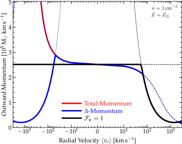
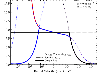
Figure 1: Momentum associated with different definitions of $\mathcal{F}_{\bf v}$, as a function of the mean radial velocity of gas around a SNe $\langle v_{r}\rangle$. We assume $E_{0}=10^{51}\,{\rm erg}$; $\langle M_{\rm coupled}\rangle\sim 10^{6}\,{\rm M_{\odot}}$ (the results are insensitive so long as this is larger than the “cooling mass” $\sim 2000\,{\rm M_{\odot}}$); and $n=1\,{\rm cm^{-3}}$, $Z=Z_{\odot}$ (left) or $n=0.01\,{\rm cm^{-3}}$, $Z=0.01\,Z_{\odot}$ (right), with $\beta_{\Lambda}\approx 0.5$ for Bremsstrahlung cooling. We compare three choices of $\mathcal{F}_{\bf v}$: (1) that given by the “total momentum change” between pre-SNe and asymptotic post-SNe states (§ 3.1), (2) the alternative “$\Delta$-Momentum” (difference in non-linear states with and without a SNe; § 3.2), or (3) simply taking $\mathcal{F}_{\bf v}\rightarrow 1$. For each we show the energy-conserving $p_{\rm egy}$ or $\Delta p_{\rm egy}$, “terminal” momentum $p_{\rm term}$, and minimum (coupled $p_{0}$; Eq. 1). For $\langle v_{r}\rangle\gtrsim-10\,{\rm km\,s^{-1}}$, the behaviors are similar, but they differ dramatically in converging flows.

In the last decade, an increasingly popular method (at least in resolved-ISM simulations with cold neutral media and mass resolution $\lesssim 10^{6}\,{\rm M_{\odot}}$) to address this dilemma is to implement mechanical feedback models which couple both thermal and kinetic energy/momentum (see e.g. Hopkins et al., 2012a, 2014, 2018b, 2023; Kimm & Cen, 2014; Agertz & Kravtsov, 2015; Rosdahl et al., 2017; Hu et al., 2017; Read et al., 2017; Lupi et al., 2017; Kim & Ostriker, 2017; Marinacci et al., 2019; Lahén et al., 2020; Agertz et al., 2021; Martin-Alvarez et al., 2022). Most of these algorithms reflect some variant of those in Hopkins et al. (2012a, 2014), where the momentum coupled is scaled with the resolution/coupling scale in order to represent the “PdV” work done by the hot SNe bubble in whatever energy-conserving phase is un-resolved – the so-called “terminal momentum” $p_{\rm term}$. This terminal momentum has since been extensively studied in orders-of-magnitude higher resolution simulations including the effects of different ambient density, metallicity, magnetic fields, SNe energy, multiple clustered SNe, pre-SNe feedback, and surrounding gas turbulence (Hennebelle & Iffrig, 2014; Iffrig & Hennebelle, 2015; Martizzi et al., 2015; Walch & Naab, 2015; Kim & Ostriker, 2015; Haid et al., 2016; Gentry et al., 2017, 2019; Ohlin et al., 2019; El-Badry et al., 2019; Zhang & Chevalier, 2019; Pittard, 2019), which in general have found it varies only weakly with these parameters, and agrees surprisingly well with classic, simple analytic models (e.g. Chevalier, 1974). In the meantime, numerical improvements to these algorithms have been developed (Hopkins et al., 2018a, 2023) which allow for such coupling to manifestly ensure mass, momentum, and energy conservation as well as the translational, Galilean, and rotational symmetries intrinsic to the problem and avoid imprinting spurious effects such as preferred grid directions.

As discussed in Hopkins et al. (2023), ensuring exact total energy conservation in the SNe coupling operation requires that the effective total momentum coupled in the low-resolution limit depend, at least in some cases, on the surrounding velocity field – i.e. $p_{\rm term}$ cannot remain very weakly velocity-dependent for arbitrary surrounding velocity fields. This becomes important in a regime which most of the idealized simulations above did not explore, namely when there is a large net velocity divergence (inflow/outflow or converging/diverging flow $\langle v_{r}\rangle$) around a given SNe (although this effect was noted for SNe in pre-existing outflows in some studies above, such as Pittard 2019). Indeed most of the high-resolution studies cited which did not assume an initially stationary ambient medium considered a uniformly turbulent medium, so the net inflow+outflow around a median SNe cancel and the effect discussed here is small (see discussion in Hopkins et al., 2018a). As a result, the vast majority of the prescriptions cited above and used in galaxy-formation simulations above simply adopt a constant $p_{\rm term}$, regardless of the true solution velocity dependence or energy conservation considerations.

In this paper, we therefore consider this question in more detail, and show that an important ambiguity arises when SNe explode in strongly-converging flows. While this may not be relevant for the “median” SNe, we show that it can have a large effect on galaxy formation (at typically-adopted numerical resolution) if standard analytic models for the terminal momentum and blastwave evolution are extended to media with non-vanishing $\langle v_{r}\rangle$. We show that this can explain some surprisingly large differences between galaxy formation simulations with seemingly similar physics, and motivate further idealized simulations for the regime of strong converging flows. In the process, we present a more simplified and flexible version of the manifestly-conservative SNe algorithm from Hopkins et al. (2018a, 2023), which we make public in the code GIZMO.

2 Supernova Coupling

Consider a simulation where a mechanical feedback “event” occurs and we wish to couple a combination of energy and momentum to the surrounding cells following Hopkins et al. (2018a) and Hopkins et al. (2023) as detailed in Appendix A. Numerically, this manifestly ensures isotropy and translation, Galilean, and rotation invariance plus mass, momentum, and energy conservation. The total radial/outward momentum coupled (in the frame of the star) is:

$$p_{0} ={\rm MIN}[p_{\rm egy}\ ,\ p_{\rm term}]$$ (1)

where $p_{\rm egy}\equiv\psi\,p_{\rm ej}$ (in terms of the ejecta momentum $p_{\rm ej}=m_{\rm ej}\,v_{\rm ej}$ and $\psi$ defined in Appendix A) is the momentum of a strictly energy-conserving Sedov solution, and $p_{\rm term}$ is some limiting or “terminal” momentum. Since we are interested in SNe (which carry most of the energy and momentum), we follow Hopkins et al. (2023) and for non-SNe (e.g. stellar mass-loss) simply set $p_{\rm term}\rightarrow p_{\rm ej}$.

For SNe, the important “sub-grid physics” is contained, by construction, in the function $p_{\rm term}$, which is some function of ambient gas properties, themselves estimated self-consistently from the surrounding cells (Appendix A). For simplicity, assume a separable function of the form:

$$p_{\rm term} =p_{t,\,0}\,\mathcal{F}_{\mathcal{E}}(\mathcal{E})\mathcal{F}_{n}(\langle n\rangle)\,\mathcal{F}_{Z}(\langle Z\rangle)\,\mathcal{F}_{\bf v}(\langle{\bf v}\rangle)$$ (2)

In terms of the total SNe-frame ejecta energy $\mathcal{E}$, and gas density $\langle n\rangle$, metallicity $\langle Z\rangle$, and velocity field $\langle{\bf v}\rangle={\bf v}_{\rm gas}({\bf x}-{\bf x}_{\ast})-{\bf v}_{\ast}$. Our “reference” scalings assumed in Hopkins et al. (2023) are: $\mathcal{F}_{\mathcal{E}}=\mathcal{E}/10^{51}\,{\rm erg}$; $\mathcal{F}_{n}(\tilde{n}\equiv\langle n\rangle/{\rm cm^{-3}})=2.63$ for $\tilde{n}<0.001$ and $=\tilde{n}^{-0.143}$ for $\tilde{n}\geq 0.001$; $\mathcal{F}_{Z}(\tilde{z}\equiv Z/Z_{\odot})=2$ for $\tilde{z}<0.01$, $=\tilde{z}^{-0.18}$ for $0.01\leq\tilde{z}\leq 1$ and $=\tilde{z}^{-0.12}$ for $\tilde{z}>1$; and $p_{t,\,0}/{\rm M_{\odot}\,km\,s^{-1}}=(f_{\rm kin}^{0})^{1/2}\,4.8\times 10^{5}\approx 2.5\times 10^{5}$. We can also write $p_{\rm term}=(\mathcal{E}/v_{\rm term})\,\mathcal{F}_{{\bf v}}$ with $v_{\rm term}\approx 200\,{\rm km\,s^{-1}}\,\mathcal{F}_{n}^{-1}\,\mathcal{F}_{Z}^{-1}$.

The scalings for $p_{t,\,0}$, $\mathcal{F}_{\mathcal{E}}$, $\mathcal{F}_{n}$, and $\mathcal{F}_{Z}$ are relatively well-understood: they can be derived both analytically and empirically from numerical simulations as the result of where SNe explosions will efficiently cool (see references in § 1), and are weak. The poorly-understood scaling, and our main focus, is the function $\mathcal{F}_{\bf v}$.

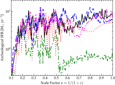
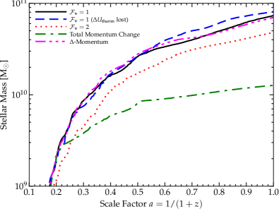
Figure 2: Effects of different terminal momentum choices in cosmological simulations (§ 4). We compare otherwise identical cosmological simulations of a Milky Way-mass halo at $z=0$ with FIRE-3, varying $\mathcal{F}_{\bf v}$, at intermediate resolution ($\langle\Delta m\rangle\sim 6\times 10^{4}\,{\rm M_{\odot}}$) We show the archeological SF history and stellar mass growth. At this resolution individual SNe cooling radii are unresolved, so systematically changing the terminal momentum via $\mathcal{F}_{\bf v}$ directly renormalizes the SFR. Using the “total momentum change” (§ 3.1) formulation leads to a very strong suppression of SF at late times (once the potential becomes deep enough that with fixed $\mathcal{F}_{\bf v}\sim 1$, inflows would become stronger). Using a fixed $\mathcal{F}_{\bf v}=1$ or $\mathcal{F}_{\bf v}$ from the “$\Delta$-Momentum” formulation (§ 3.2) give similar results.

3 How Should the Terminal Momentum Depend on Velocity?

3.1 A First Guess: The “Total” Change in Momentum

Of course, on the size scale of the SNe blastwave and coupling to the gas, the “true” velocity field could be infinitely complex, and ultimately understanding $\mathcal{F}_{\bf v}$ requires numerical simulations. But we wish to gain some intuition with simple models. If we write the smooth (on this scale) large-scale velocity field as ${\bf v}\approx\langle{\bf v}\rangle+\langle\nabla{\bf v}\rangle\cdot{\bf x}+\mathcal{O}({\bf x}^{2})$ (in the frame of the star), and decompose $\nabla{\bf v}$ into the usual trace-free/deviatoric shear, rotation, and expansion/compression ($\nabla\cdot{\bf v}\sim\langle v_{r}\rangle/r$) terms, we can gain some insight. Since our SNe solutions assume spherical symmetry, the only of these terms which should enter is the $\nabla\cdot{\bf v}\rightarrow r^{-2}\,\partial_{r}(r^{2}\,v_{r})$, i.e. $v_{r}$ term. In § B we re-derive the usual analytic terminal momentum argument by considering the radius at which a spherically-symmetric blastwave would have its cooling time fall below its dynamical time, now allowing for a uniform radial velocity $\langle v_{r}\rangle$ in the frame of the star, and show the result can be approximated as $\mathcal{F}_{\bf v}\approx 1/(1+\langle v_{r}\rangle/v_{\rm term})$.

For $\langle v_{r}\rangle\geq 0$, this gives completely reasonable behavior. At small $\langle v_{r}\rangle\rightarrow 0$, $\mathcal{F}_{\bf v}\rightarrow 1$, as it should, and for $\langle v_{r}\rangle\gg v_{\rm term}$, $\mathcal{F}_{\bf v}\rightarrow v_{\rm term}/\langle v_{r}\rangle$ and $p_{\rm term}\rightarrow E_{0}/\langle v_{r}\rangle$. But this is the same behavior as $p_{\rm egy}$ at large $\langle v_{r}\rangle$ (because both reflect the same total energy; § A.3). So it is functionally identical to assume $\mathcal{F}_{{\bf v}}=1$ for all $\langle v_{r}\rangle\geq 0$.

The important difference arises for negative $\langle v_{r}\rangle<0$, i.e. net infall towards the SNe. The simple expression above gives $\mathcal{F}_{\bf v}\rightarrow\infty$ for $\langle v_{r}\rangle\leq v_{\rm term}$, and while the more detailed expressions in § B do not formally diverge, they give effectively the same result, with $\mathcal{F}_{\bf v}\sim|\langle v_{r}\rangle/v_{\rm term}|^{14}$ or so for $\langle v_{r}\rangle\ll-v_{\rm term}$. In practice, this means that in this limit one never reaches the “terminal” momentum, because the inflowing gas velocity ensures the post-shock temperature is so hot that cooling is inefficient, and the coupling will be determined by the energy-conserving solution $p_{\rm egy}$. But that solution in this limit gives $p_{\rm egy}\rightarrow-2\,\langle M_{\rm coupled}\rangle\langle v_{r}\rangle$ ($\psi\rightarrow-2\,\beta_{1}/\beta_{2}=-2\,(\langle v_{r}\rangle/v_{\rm ej})\,(\langle M_{\rm coupled}\rangle/m_{\rm ej})$; § A.3). So the inflow is always halted and reversed, with the peculiar feature that the coupled momentum becomes independent of the input energy even as $E_{0}\rightarrow 0$.

This is not some unique artifact of assumptions we adopted: we obtain the same qualitative result if we instead approximate the blastwave as occurring in a Hubble flow, or isothermal inflow/wind solution, or even as a one-dimensional surface with some external inflow (see solutions in Ostriker & McKee, 1988); whether we consider the shell approximation or a homogenous sphere, and whether we consider the energy injection as impulsive or continuous over the timestep; whether we consider the ambient medium to be infinite, or strictly limited to the mass $\langle M_{\rm coupled}\rangle$; or whether we vary the cooling curve ($\beta_{\Lambda}$ in § B). The reason is simple: in this limit of a spherically-symmetric inflow with inflow kinetic energy much larger than ejecta energy ($\langle M_{\rm coupled}\rangle\langle v_{r}\rangle^{2}\gg E_{0}$), the problem transitions fundamentally from a “blastwave” to an “accretion shock.” Our analytic solutions are qualitatively completely reasonable when we realize they are the standard solutions for an accretion shock, which when $\langle v_{r}\rangle\ll-v_{\rm term}$ corresponds to post-shock cooling times which are long (e.g. “hot” halos) and so the shocked region grows as the mass supply continues (Rees & Ostriker, 1977).

3.2 An Alternative: The Change in Total Momentum Relative to Evolution Without Feedback

This explains the seemingly strange behavior of $p_{\rm term}$ and $p_{\rm egy}$, but highlights what is problematic about our approach for $\langle v_{r}\rangle\ll 0$: by applying the “final” momentum (energy-conserving or terminal) in this limit, we are essentially “jumping ahead” of the hydro/MHD solver. If, after all, $\langle v_{r}\rangle\ll-v_{\rm term}$, then there is sufficient energy in the resolved simulation cells to heat themselves above the threshold where cooling is inefficient, so this solution should be resolved. Thus while not technically wrong or unphysical (or in violation of any conservation law), this “jumping ahead” can be problematic for several reasons: (1) we are making many approximations (like spherical symmetry, an idealized cooling function, no other sources/sinks, a single blastwave in isolation, homogeneous and isotropic density/metallicity/velocity fields, no radiation or cosmic rays or other forces, etc.) which the actual surrounding gas may not obey, (2) it is possible that this “jumping ahead” could effectively jump to a solution further in time than the actual code timestep would allow (if e.g. the gas on either side of the SNe should not be able to “cross” and shock yet in the timestep during which the SNe is coupled), and (3) it violates the spirit of a well-posed sub-grid model, in that such should represent the result of only un-resolved processes but “trust” the code for dealing with resolved processes.

A potential alternative is instead to apply the “$\Delta$-Momentum”: specifically, instead of calculating the final momentum injected in a SNe $p_{0}$ as the difference between the initial (pre-SNe) code momentum state $p_{\rm initial}$ and some analytic “post-evolution” blastwave/shock state $p_{\rm final}$ ($p_{0}=p_{\rm final}-p_{\rm initial}$), we can define the $\Delta$-Momentum $\Delta p$ as the difference between these states relative to the solution where there is no SNe at all (mathematically $\Delta p\equiv(p_{\rm final}-p_{\rm initial})_{E_{0}=E_{0}}-(p_{\rm final}-p_{\rm initial})_{E_{0}\rightarrow 0}$), in order to identify how said SNe uniquely modifies the state. These solutions are derived in § B.2. Fig. 1 compares the behavior of the naive final momentum coupled $p_{0}$ and the $\Delta$-Momentum $\Delta p$ for realistic simulation conditions. For both the energy-conserving and terminal limit, the $\Delta$-Momentum is identical to the “normal” final momentum we would have coupled above, $\Delta p=p_{0}$, for $\langle v_{r}\rangle\geq 0$. But for $\langle v_{r}\rangle<0$, there is longer any divergence in momentum coupled, $\Delta p$ vanishes as $E_{0}\rightarrow 0$, and for very large $\langle v_{r}\rangle\ll-v_{\rm term}$, $\Delta p\propto 1/|\langle v_{r}\rangle|$ is a decreasing function of $|\langle v_{r}\rangle|$ (it no longer grows without limit). But we should stress that since the equations being represented here are fundamentally non-linear, it is by no means obvious that the sum of the ad-hoc defined $\Delta$-Momentum plus subsequent resolved solution evolution in-code will actually give the same non-linear answer as a direct solution at much higher resolution.

Given this ambiguity and the range “bracketed” by the above final momentum and $\Delta$-momentum, an even simpler alternative is just to always take $\mathcal{F}_{{\bf v}}=1$. We see in Fig. 1 that for $\langle v_{r}\rangle\geq 0$, this is basically identical to either of these more sophisticated approaches, but for $\langle v_{r}\rangle\lesssim-v_{\rm term}$, it is “in between.”

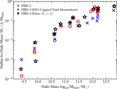
Figure 3: Comparison of the stellar mass-halo mass relation at $z=0$ from cosmological simulations (§ 4). We plot total stellar mass (within $<20\,$kpc of the halo center) versus halo virial mass for each primary galaxy in a zoom-in region, for identical initial conditions simulated with FIRE-3 adopting the SNe treatment here with $\mathcal{F}_{\bf v}=1$; or using the treatment assumed in Hopkins et al. (2023, H23), which was similar to the “Total Momentum Change” formula for $\mathcal{F}_{\bf v}$ with a “cap” at $\mathcal{F}_{\bf v}\lesssim|\bar{\bf w}_{ba}|^{-1/2}\sim$ a few; and FIRE-2 (Hopkins et al., 2018a), which adopted $\mathcal{F}_{\bf v}=1$ but a different and not strictly energy-conserving SNe coupling, different cooling physics, stellar evolution tables, yields, treatment of OB/AGB mass-loss, UV background, and star formation criteria. Details of the differences between SNe treatments are in § C. These are hydrodynamics-only (no MHD or cosmic rays), no-AGN, low-resolution simulations (resolution $\sim(300,\,10^{4},\,6\times 10^{4},\,3\times 10^{5})\,{\rm M_{\odot}}$ for $M_{\rm halo}\sim(10^{10},\,10^{11},\,10^{12},\,10^{13})\,{\rm M_{\odot}}$). The different H23 and FIRE-2 predictions for stellar masses in massive ($M_{\rm halo}\gg 10^{11}\,{\rm M_{\odot}}$) galaxies appears to be dominated by the implicit difference in $\mathcal{F}_{\bf v}$.

4 Effects in Galaxy Formation Simulations

We now consider the effects of these choices in cosmological galaxy formation simulations. The specific simulations we consider below were run as part of the Feedback In Realistic Environments (FIRE) project, specifically using the FIRE-3 version of the code; all details of the methods are described in Hopkins et al. (2023). Briefly, the simulations use the code GIZMO (Hopkins, 2015), with hydrodynamics solved using the mesh-free Lagrangian Godunov MFM method. Both hydrodynamic and gravitational (force-softening) spatial resolution are set in a fully-adaptive Lagrangian manner; mass resolution is fixed. The simulations include cooling and heating from a meta-galactic background and local stellar sources from $T\sim 10-10^{10}\,$K; SF in locally self-gravitating and Jeans-unstable gas; and stellar feedback from OB & AGB mass-loss, SNe Ia & II, and multi-wavelength photo-heating and radiation pressure; with inputs taken directly from stellar evolution models. We compare a set of fully-cosmological zoom-in simulations run from initial redshifts $z\sim 100$ down to $z=0$ with fiducial resolution surrounding a “target” halo of interest. Here, we keep the physics and numerical methods identical to those in Hopkins et al. (2023), and vary only mechanical coupling, using the exact numerical prescription from Appendix A, with the important physical variations contained in the function $\mathcal{F}_{{\bf v}}$.

Fig. 2 compares the history of a typical Milky Way-mass galaxy (m12i from Hopkins et al. 2014), for several choices of $\mathcal{F}_{{\bf v}}$. This simulation has a modest, but common for “zoom-in” cosmological simulations, mass resolution of $\langle m_{b}\rangle\sim 6\times 10^{4}\,{\rm M_{\odot}}$, which as noted in the Appendices gives $\langle M_{\rm coupled}\rangle\sim(2-4)\times 10^{5}\,{\rm M_{\odot}}$, so as a result is almost always in the “terminal momentum” limit. We therefore see the expected result from feedback-regulated SF, consistent with many previous more systematic studies with the FIRE simulations (e.g. Hopkins et al., 2011, 2012b; Orr et al., 2018; Pandya et al., 2021), that the average SFR and final stellar mass are approximately inversely proportional to the strength of feedback, which here is dominated by SNe with un-resolved cooling radii so essentially given by $p_{\rm term}$ and hence $\mathcal{F}_{{\bf v}}$.

These results are entirely expected if we change $\mathcal{F}_{{\bf v}}$ systematically – what is more interesting is if we look at how $\mathcal{F}_{{\bf v}}$ varies with $\langle v_{r}\rangle$. If we adopt the “total momentum change” formalism, we see a strong suppression of SF, particularly at late times. This is because, as discussed in Hopkins et al. (2023), when stellar feedback normally would become less efficient in higher galaxy/halo masses and deeper potentials, the system will more and more often show gas in inflow around a SNe, which then strongly boosts its efficiency, so this decreasing feedback efficiency is partially offset. Changing, on the other hand, the residual thermal coupling of the gas has almost no effect, because at this resolution the cooling radii are unresolved.

Fig. 3 extends this to compare the stellar mass-halo mass relation from the same simulations, with halos masses spanning $\sim 10^{9}-10^{13}\,{\rm M_{\odot}}$ and stellar masses $\sim 10^{4}-10^{12}\,{\rm M_{\odot}}$. For halo masses $\lesssim 10^{11}\,{\rm M_{\odot}}$, we see weaker effects of $\mathcal{F}_{{\bf v}}$, for two reasons: (1) the resolution of these isolated dwarf zoom-ins is higher (see Table 1 in Hopkins et al. 2018b), reaching $\sim 10^{2}\,{\rm M_{\odot}}$ for the smallest, so the cooling radii are increasingly resolved; and (2) because feedback in dwarfs is so strong, a much larger fraction of SNe explode in super-bubbles with $\langle v_{r}\rangle\gg 0$ (where $\mathcal{F}_{\bf v}$ is similar in all tested prescriptions). We also compare the results from FIRE-2 (Hopkins et al., 2018b), which effectively assumed $\mathcal{F}_{\bf v}=1$, but also a different numerical SNe implementation, UV background, cooling and thermo-chemistry, stellar evolution tables, and more; as well as the initial FIRE-3 runs from Hopkins et al. (2023), which adopted $\mathcal{F}_{\bf v}$ closer to the “total momentum change” model but are otherwise similar to our runs here (see § C). In dwarfs, the difference between FIRE-2 and FIRE-3 is robust owing to the various changes above (and less sensitive to $\mathcal{F}_{\bf v}$, though it can be sensitive to the energy-conserving terms $\psi$; Hopkins et al. 2023), but we see that the substantial difference between FIRE-2 and the Hopkins et al. (2023) runs at halo masses $\gtrsim 10^{11}\,{\rm M_{\odot}}$ can primarily be attributed to the implicit choice of $\mathcal{F}_{\bf v}$.

5 Conclusions

In galaxy formation simulations, it is common to treat SNe feedback with a subgrid model for kinetic and thermal injection representing the work done in any unresolved energy-conserving phase. We show that extending such treatments to be “velocity-aware” (i.e. dependent on the velocity field of gas surrounding the SNe, as required for strict energy conservation) introduces an ambiguity when SNe explode in converging flows. In this limit, there are a range of allowed (fully-conservative and analytically justifiable) sub-grid solutions, which differ strongly in how much momentum is imparted to the gas. This dependence is much stronger than the reasonably well-understood dependence of momentum coupled on ambient gas density, metallicity, or turbulence. We show that this can produce significant differences in cosmological galaxy-formation simulations, especially in high-mass galaxies at low resolution. We also stress that this is a physical, rather than numerical, ambiguity. As such, even in simulations which numerically couple feedback in a qualitatively different manner (e.g. “delayed cooling” models which do not explicitly couple momentum), the same fundamental ambiguity exists of how to scale mechanical feedback with surrounding gas velocities.

Given this intrinsic physical ambiguity and the absence of clear guidance from simulations which resolve individual SNe explosions in the relevant environments, we would recommend future work adopt the simplest possible model, namely our “$\mathcal{F}_{{\bf v}}=1$” formulation, as it introduces no additional implicit assumptions and is straightforward to compare to both previous simulations and idealized models. And as we showed this gives similar results in galaxy-formation simulations (at least for bulk galaxy properties) to the “$\Delta$-Momentum” formulation. But clearly, an important path for future work is to study the ambiguous cases here in more detail in higher-resolution simulations to develop more accurate sub-grid models for the extreme, but sometimes relevant limits. We have shown that is important for such models to not simply quantify the final momentum state or “total” momentum change of the high-resolution simulation, as is usually done, but to think carefully about the change in this state specifically introduced at a given spatial, mass, and time scale by individual SNe as a function of their local properties, so that this can be implemented in sub-grid models without “skipping over” resolved MHD processes.

Appendix A Conservative Coupling of Mechanical Feedback

A.1 Coupling Equations

Following Hopkins et al. (2018a) and Hopkins et al. (2023), consider an “event” where a star particle “$a$” (with coordinate position ${\bf x}_{a}$, velocity ${\bf v}_{a}$, total particle/cell mass $m_{a}$) injects, in a given timestep $\Delta t$ (taking the code from initial time $t^{(0)}\rightarrow t^{(1)}=t^{(0)}+\Delta t$), some ejecta mass $m_{{\rm ej},\,a}$ (which can be spread across different explicitly-followed species “$s$,” as $m_{{\rm ej},\,a}\equiv\sum_{s}m_{{\rm ej},\,a,\,s}$). In the rest-frame of the star particle, assume the ejecta is isotropic with total kinetic energy ${\rm KE}_{{\rm ej},\,a}$ (and some arbitrary set of scalar energies “$j$” including e.g. thermal and cosmic ray and radiation energies $U_{{\rm ej},\,a,\,j}$). The ejecta is coupled to some set of gas cells “$b$,” which consist of all cells for which there is a non-vanishing oriented hydrodynamic face area ${\bf A}_{ba}$ that can be constructed between them and the star particle $a$ (this is defined rigorously in Hopkins et al. (2018a), but essentially includes all cells $b$ which are either “neighbors of $a$” or for which “$a$ is a neighbor of $b$”). Given a single event site $a$, then the update to the conserved quantities (e.g. $m$, $U$, and momentum ${\bf p}$) of cell $b$ is given by:

$$m_{b,\,s}^{(1)} =m_{b,\,s}^{(0)}+|\bar{\bf w}_{ba}|\,m_{{\rm ej},\,a,\,s}$$ (3)

$$U_{b,\,j}^{(1)} =U_{b,\,j}^{(0)}+|\bar{\bf w}_{ba}|\,U_{{\rm ej},\,a,\,j}$$

$${\bf p}_{b}^{(1)} ={\bf p}_{b}^{(0)}+\Delta m_{ba}\,{\bf v}_{a}+\Delta{\bf p}_{ba}$$

$$\Delta{\bf p}_{ba} \equiv\bar{\bf w}_{ba}\,p_{0,\,a}$$

Here $\Delta m_{ba}\equiv|\bar{\bf w}_{ba}|\,m_{{\rm ej},\,a}$ and $\bar{\bf w}_{ba}$ is a normalized vector weight function defined in Hopkins et al. (2018a). As shown therein, this ensures all the desired symmetries (e.g. isotropy in the frame of the star and $\sum_{b}|\bar{\bf w}_{ba}|=1$) as well as mass ($\sum_{b}\sum_{s}|\bar{\bf w}_{ba}|\,m_{{\rm ej},\,a,\,s}=\sum_{b}\Delta m_{ba}=m_{{\rm ej},\,a}$) and linear momentum conservation ($\sum_{b}\Delta{\bf p}_{ba}=\mathbf{0}$), with the total coupled radial momentum equal to $p_{0,\,a}$ in the star frame ($\sum_{b}|\Delta{\bf p}_{ba}|=p_{0,\,a}$).

A.2 Enforcing Total Energy Conservation

Without loss of generality, define

$$p_{0,\,a} \equiv\psi_{a}\,\chi_{a}\,(2\,\epsilon_{a}\,m_{{\rm ej},\,a})^{1/2}$$ (5)

in terms of some effective unit of kinetic energy

$$\epsilon_{a} \equiv f_{\rm kin}^{0}\,\mathcal{E}_{a}\equiv(1-f_{U}^{0})\mathcal{E}_{a}\,$$ (6)

$$\mathcal{E}_{a} \equiv E_{{\rm ej},\,a}+\frac{1}{2}\sum_{b}m_{{\rm ej},\,a}\,w^{\prime}_{ba}\,|{\bf v}_{ba}|^{2}$$

where $E_{{\rm ej},\,a}$ is the total ejecta energy (in the frame of the star, ignoring any surrounding gas), and $f_{U}^{0}$ and $f_{\rm kin}^{0}=1-f_{U}^{0}$ are the fraction of the total energy in thermal (or other, e.g. radiation, cosmic rays, etc.) versus kinetic, fixed (hence the ⁰ superscript) to their values for e.g. an idealized Sedov (1959) solution in a homogeneous background, $f_{\rm kin}^{0}=0.28$. At this stage, this is just a choice of units. As shown in Hopkins et al. (2018a), the exact, discrete total energy conservation equation is:

$$\epsilon_{a} =\sum_{b}\,\left[\frac{|\Delta{\bf p}_{b}|^{2}}{2\,m_{b}\,(1+\mu_{b})}+\frac{{\bf v}_{ba}\cdot\Delta{\bf p}_{b}}{(1+\mu_{b})}\right]$$ (7)

which becomes (inserting our definition of $\Delta{\bf p}_{b}$):

$$\frac{(\mathcal{E}_{a}-U_{a})}{\epsilon_{a}} =(\psi_{a}\,\chi_{a})^{2}\,\beta_{2,\,a}+2\,(\psi_{a}\,\chi_{a})\,\beta_{1,\,a}$$ (8)

$$\frac{\langle v_{r}\rangle_{a}}{v_{{\rm ej},\,a}} \equiv\beta_{1,\,a}\equiv\left(\frac{m_{{\rm ej},\,a}}{2\,\epsilon_{a}}\right)^{1/2}\,\sum_{b}w^{\prime}_{ba}\,{{\bf v}_{ba}\cdot\hat{\bf w}_{ba}}$$ (9)

$$\frac{m_{{\rm ej},\,a}}{\langle M_{\rm coupled}\rangle_{a}} \equiv\beta_{2,\,a}\equiv m_{{\rm ej},\,a}\,\sum_{b}\frac{w^{\prime}_{ba}\,|\bar{\bf w}_{ba}|}{m_{b}}$$ (10)

where ${\bf v}_{ba}\equiv{\bf v}_{b}-{\bf v}_{a}$.

Now, consider the case where the ejecta are in a purely energy-conserving Sedov-Taylor type phase, with some analytically-calculated (fixed/self-similar) ratio of kinetic to total energy $f_{\rm kin}^{0}$, where $\mathcal{E}_{a}$ represents the total energy available to the blastwave, and $U_{a}$ represents the fraction in non-kinetic sources, $U_{a}=f_{U}\,\mathcal{E}_{a}\rightarrow f_{U}^{0}\,\mathcal{E}_{a}$. Then clearly the left-hand side of Eq. 8 becomes unity ($\rightarrow 1$). Moreover given its strict degeneracy with $\psi_{a}$ we can take $\chi_{a}\rightarrow 1$ without loss of generality for now. It is then straightforward to solve and obtain the energy-conserving value of $\psi_{a}$:

$$\psi_{a} \equiv\frac{\sqrt{\beta_{2,\,a}+\beta_{1,\,a}^{2}}-\beta_{1\,a}}{\beta_{2,\,a}}$$ (11)

$$=\frac{1}{\beta_{2,\,a}^{1/2}}\left[\sqrt{1+\left(\frac{\beta_{1,\,a}}{\beta_{2,\,a}^{1/2}}\right)^{2}}-\frac{\beta_{1,\,a}}{\beta_{2,\,a}^{1/2}}\right]\ .$$

The additional term $0\leq\chi_{a}\leq 1$ then allows us to represent cases with less momentum coupled (more of the energy going into some other form). If we arbitrarily define some maximal or “terminal” momentum $p_{\rm term}$, then we simply impose:

$$\chi_{a} \rightarrow{\rm MIN}\left[1\ ,\ \frac{p_{\rm term}}{\psi_{a}\,(2\,\epsilon_{a}\,m_{{\rm ej},\,a})^{1/2}}\right]$$ (12)

which then determines the value of $f_{U}\neq f_{U}^{0}$, or $U_{a}$:

$$\frac{U_{a}}{\mathcal{E}_{a}} =1-\left[(\psi_{a}\,\chi_{a})^{2}\,\beta_{2,\,a}+2\,(\psi_{a}\,\chi_{a})\,\beta_{1,\,a}\right]\frac{\epsilon_{a}}{\mathcal{E}_{a}}$$ (13)

This will ensure that the correct total energy is always coupled. We enforce the same timestepping and parallel communication/summation rules as described in Hopkins et al. (2023) (Appendix B3) to ensure that multiple events acting on the same cell in the same timestep do not lead to spurious violations of conservation.

A.3 Limiting Behaviors

The coupled momentum Eq. 5 has four limiting behaviors.

• If $\chi<1$ ($p_{\rm term}<\psi_{a}\,(2\,\epsilon_{a}\,m_{{\rm ej},\,a})^{1/2}$), then

  $$p_{0,\,a}\rightarrow p_{\rm term}$$ (14)

  by construction. This is the “terminal momentum” limit.

• For $\chi=1$, if $\beta_{1,\,a}^{2}/\beta_{2,\,a}\ll 1$, $\psi_{a}\rightarrow\beta_{2,\,a}^{-1/2}=\sqrt{\langle M_{\rm coupled}\rangle/m_{\rm ej}}$, so the total coupled momentum is

  $$p_{0}\rightarrow\psi\,p_{\rm ej}\rightarrow\sqrt{2\,\epsilon_{a}\langle M_{\rm coupled}\rangle}$$ (15)

  (noting $p_{\rm ej}=\sqrt{2\,\epsilon_{a}\,m_{{\rm ej},\,a}}$). This is the expectation for an energy-conserving solution in a homogeneous, non-moving medium.

• For $\chi=1$, if $\beta_{1,\,a}^{2}/\beta_{2,\,a}\gg 1$, the behavior depends on the sign of $\beta_{1,\,a}\propto\langle v_{r}\rangle$. If $\langle v_{r}\rangle>0$ (the gas is net receding from the star), $\psi\rightarrow 1/2\beta_{1}$ and

  $$p_{0} \rightarrow\frac{v_{\rm ej}}{2\langle v_{r}\rangle}\,m_{\rm ej}\,v_{\rm ej}=\frac{\epsilon_{a}}{\langle v_{r}\rangle}$$ (16)

  $$=\sqrt{2\,\epsilon_{a}\langle M_{\rm coupled}\rangle}\sqrt{\frac{\epsilon_{a}}{2\langle M_{\rm coupled}\rangle\,\langle v_{r}\rangle^{2}}}$$

  Note that whether we are in this regime depends on the ratio $\beta_{1}^{2}/\beta_{2}=\langle M_{\rm coupled}\rangle\,\langle v_{r}\rangle^{2}/m_{\rm ej}\,v_{\rm ej}^{2}\sim{\rm KE}^{\rm coupled}_{r}/{\rm KE}_{\rm ej}$, i.e. just the ratio of the pre-existing radial kinetic energy of the background gas to the ejecta kinetic energy. When this is large, the coupled momentum is suppressed relative to the energy-conserving solution in a non-moving background by the root of this factor, to enforce total energy conservation, since the coupled kinetic energy is a non-linear function of the coupled momentum.

• If $\chi=1$, $\beta_{1,\,a}^{2}/\beta_{2,\,a}\gg 1$, and $\langle v_{r}\rangle<0$ (the gas is net infalling towards the star), then $\psi\rightarrow-2\,\beta_{1}/\beta_{2}$ and

  $$p_{0}\rightarrow-2\,\langle M_{\rm coupled}\rangle\,\langle v_{r}\rangle$$ (17)

  In this limit, from a purely energetic point of view, since there is an enormous energy reservoir in the inflow kinetic energy, there can always be enough energy to reverse the inflow to outflow with similar $|v_{r}|$. In practice, the physics of these cases will be regulated by our scaling of $p_{\rm term}$.

A.4 Quantities Determining the Terminal Momentum

The terminal momentum $p_{\rm term}$ can be a function of various properties of the ambient gas and ejecta itself, e.g.

$$p_{\rm term}=p_{\rm term}(\langle\boldsymbol{\Upsilon}_{a}\rangle\ ,\ \boldsymbol{\Psi}_{a})$$ (18)

where

$$\langle{\Upsilon}_{a,\,j}\rangle\equiv\sum_{b}|\bar{\bf w}_{ba}|\,{\Upsilon}_{b,\,j}$$ (19)

and $\boldsymbol{\Upsilon}_{b}=\{n_{b},\,Z_{b},\,T_{b},\,....\}$ is determined by various scalar properties of the neighboring gas cells, weighted appropriately by the fraction of the ejecta $|\bar{\bf w}_{ba}|$ associated with each cell (and $\boldsymbol{\Psi}_{a}$ represents intrinsic ejecta properties such as $\mathcal{E}_{a}$, $m_{{\rm ej},\,a}$, etc.). Given that we are assuming isotropy in the frame of the star already above in our definition of weights to ensure e.g. linear momentum conservation, we use these weighted averages at the ejecta origin, rather than solving “along cells” or cones independently (which necessarily violates said isotropy). For $p_{\rm term}$ being a non-linear function of certain properties such as $n^{\alpha_{n}}\,Z^{\alpha_{Z}}$, we take $\sum_{b}|\bar{\bf w}_{ba}|\,n_{b}^{\alpha_{n}}\,Z_{b}^{\alpha_{Z}}$, to avoid pathological behaviors caused by covariances of these quantities.

A.5 Practical Meaning of $\langle M_{\rm coupled}\rangle$

As an aside, the parameter $\langle M_{\rm coupled}\rangle\equiv\left[\sum_{b}w^{\prime}\,|\bar{\bf w}|_{ba}/m_{b}\right]^{-1}=\left[\sum_{b}|\bar{\bf w}|^{2}_{ba}/(m_{b}+|\bar{\bf w}|_{ba}\,m_{{\rm ej},\,a})\right]^{-1}\approx\left[\sum_{b}|\bar{\bf w}|^{2}_{ba}/m_{b}\right]^{-1}$ defined in Eq. 10 provides a rigorous way of thinking of the total energy change of the system, but also about the effective total mass among which the ejecta energy and momentum are shared. This is especially useful for irregular-mesh or mesh-free methods such as those employed in codes like GIZMO or AREPO where the kernel into which SNe ejecta are deposited can include some neighbors with extremely small shared face areas ${\bf A}$. Notably given the quadratic dependence on the weight function $|\bar{\bf w}|^{2}_{ba}$, these will contribute negligibly to $\langle M_{\rm coupled}\rangle$. It is straightforward to estimate analytically, and verify directly in the simulations, given the definition of face (Hopkins, 2015) and cubic spline kernel function for the volume decomposition used in the FIRE-3 GIZMO simulations plus the roughly-equal cell masses $m_{b}\approx\langle m_{b}\rangle$ presented here, that $\langle M_{\rm coupled}\rangle\sim(4-6)\times\langle m_{b}\rangle$, i.e. the effective coupled mass is a few times the median cell mass. This is quite different from some other implementations: for example the methods used in Hu et al. (2014); Hu et al. (2019), which adopt a different hydrodynamic method and face definition, kernel function, and method for depositing ejecta, which give $\langle M_{\rm coupled}\rangle\sim(100-200)\times\langle m_{b}\rangle$. That, in turn, has an important consequence for the physical limit the coupling is in – the Hu et al. (2014) method will therefore require $\sim 30\times$ better mass resolution (compared to the FIRE-2/3 method here) to begin to effectively capture the energy-conserving phase, in good agreement with the comparison of direct resolution tests presented in Hopkins et al. (2018a) and Hu et al. (2014).

Appendix B Analytic Scalings for $\mathcal{F}_{{\bf v}}$

B.1 “Absolute” Terminal Momentum Change

Consider the rest-frame of a star which explodes isotropically in an isotropic, spherically-symmetric gaseous medium with a uniform radial velocity flow (i.e. for the region of interest around the star, the velocities are radial with some roughly-constant $v_{r}$), and let us make the shell approximation and assume the swept-up mass in the shell $M_{s}\gg m_{\rm ej}$ is much larger than the initial ejecta mass (which carried some energy $E_{0}$), and that the energy is divided between kinetic and thermal forms. All of these assumptions can be freed, we simply wish to illustrate a heuristic argument here. Energy conservation (pre-cooling) gives $E_{0}+(1/2)\,M_{s}\,v_{r}^{2}\approx(1/2)\,M_{s}v_{s}^{2}+U_{\rm th}$, where the thermal energy $U_{\rm th}\approx(3/2)\,(M_{s}/\mu)\,k_{B}\,T_{s}\approx f_{U}\,(1/2)\,M_{s}\,(v_{s}-v_{r})^{2}$ with some $f_{U}=1-f_{K}$ where $0\leq f_{U}<1$ is some similarity parameter whose exact value is not important. Re-arranging this, we can solve for $v_{s}(M_{s})=v_{r}\,f_{U}/(1+f_{U})+\sqrt{2\,E_{0}/((1+f_{U})\,M_{s})+v_{r}^{2}/(1+f_{U})^{2}}$ (or equivalently $M_{s}(v_{s})$). Now define the cooling time $t_{\rm cool}=[(3/2)\,k_{B}\,T_{s}]/[(\rho_{s}/\mu)\,\Lambda(T_{s})]$, where we will approximate $\Lambda\approx\Lambda_{0}\,(T_{s}/T_{0})^{\beta_{\Lambda}}$ over the dynamic range of interest and $\rho_{s}\approx\tilde{\rho}\,\rho$ for some shock compression ratio $\tilde{\rho}$. Define the expansion time $t_{\rm exp}=r/v_{s}$ and note $r=(M_{s}/(4\pi/3)\,\rho)^{1/3}$, and it becomes possible to solve for $v_{s}$ (and hence $M_{s}$) at which $t_{\rm cool}(v_{s}=v_{s,\,c})\approx t_{\rm exp}(v_{s}=v_{s,\,c})$. Then we define the terminal momentum as $p_{\rm term}\equiv M_{s}\,v_{s}-M_{s}\,v_{r}$ (i.e. the change in momentum of the swept-up material relative to its initial value).

After some tedious algebra, the above derivation can be simplified to

$$p_{\rm term}\equiv\frac{E_{0}}{v_{\rm term}}\,\mathcal{F}_{{\bf v}}$$ (20)

where $\mathcal{F}_{{\bf v}}$ satisfies:

$$\mathcal{F}_{{\bf v}}=[(1-y)^{7/3-2\beta_{\Lambda}}\{1-(1-f_{U})\,y/2\}]^{3/(11-6\beta_{\Lambda})}$$ (21)

where $y\equiv\mathcal{F}_{{\bf v}}\,\langle v_{r}\rangle/v_{\rm term}$. This must in general be solved numerically, but the limits are simple. For small $|\langle v_{r}\rangle|/v_{\rm term}\ll 1$, $\mathcal{F}_{{\bf v}}\rightarrow 1$ (as it should). For $\langle v_{r}\rangle\gg v_{\rm term}$, $\mathcal{F}_{{\bf v}}\rightarrow v_{\rm term}/\langle v_{r}\rangle$. And for $\langle v_{r}\rangle\ll-v_{\rm term}$, $\mathcal{F}_{{\bf v}}\rightarrow[(1-f_{U})/2]^{3}\,|\langle v_{r}\rangle/v_{\rm term}|^{10-6\,\beta_{\Lambda}}$. An approximate solution accurate to $\sim 10\%$ for $\langle v_{r}\rangle\geq 0$ is $\mathcal{F}_{{\bf v}}\approx 1/[1+(1-\psi)\,\langle v_{r}\rangle/v_{\rm term}]$ with $\psi\equiv 9\,(5+3\,f_{U})/[2\,(11-6\,\beta_{\Lambda})\,(9+\langle v_{r}\rangle^{2}/v_{\rm term}^{2})]$, and a (slightly less accurate but reasonable) approximation for $\langle v_{r}\rangle<0$ is $\mathcal{F}_{{\bf v}}\approx 1+\tilde{v}_{-}+\tilde{v}_{-}^{2}+\tilde{v}_{-}^{3}+[(1-f_{U})/2]^{3}\,|\langle v_{r}\rangle/v_{\rm term}|^{10-6\,\beta_{\Lambda}}$ where $\tilde{v}_{-}\equiv(|\langle v_{r}\rangle|/v_{\rm term})\,([17-12\beta_{\Lambda}-3f_{U}]/[22-12\beta_{\Lambda}])$. Here, $v_{\rm term}\propto E_{0}^{1/11}\,n^{2/11}\,\Lambda_{0}^{3/11}$ is reasonably consistent with the simulation-calibrated $v_{\rm term}$ and its scalings $\mathcal{F}_{\mathcal{E}}$, $\mathcal{F}_{n}$, $\mathcal{F}_{Z}$ (where $Z$ appears via $\Lambda$).

We can also simplify the above by taking $\beta_{\Lambda}\rightarrow-\infty$ mathematically, or equivalently say the cooling function $\Lambda(T)$ begins to rise steeply for decreasing $T$ below some critical temperature $T_{\rm cool}$, which in turn leads to rapid cooling when the post-shock temperature $T_{s}<T_{\rm cool}$, or equivalently, which the shock-ambient medium velocity $v_{s}-v_{\rm gas}$ falls below some critical “cooling velocity” $v_{\rm cool}$. We then simply calculate $p_{\rm term}$ when $v_{s}-v_{r}=v_{\rm cool}$, which gives $p_{\rm term}=(E_{0}/v_{\rm term})\,\mathcal{F}_{{\bf v}}$ with $\mathcal{F}_{{\bf v}}\rightarrow 1/(1+\langle v_{r}\rangle/v_{\rm term})$ (making the identification $v_{\rm term}=(1+f_{U})\,v_{\rm cool}/2$) for $v_{r}>-v_{\rm term}$ and $\mathcal{F}_{{\bf v}}\rightarrow\infty$ for $v_{r}\leq-v_{\rm term}$. This has a simple closed form solution, and has the same limiting behaviors as above for $|\langle v_{r}\rangle|\ll v_{\rm term}$, $\langle v_{r}\rangle\gg v_{\rm term}$. While for $\langle v_{r}\rangle<-v_{\rm term}$ it formally diverges, the full expression above for finite $\beta_{\Lambda}$ effectively diverges as well (scaling for a more realistic $-1\lesssim\beta_{\Lambda}\lesssim 1/2$ as $|\langle v_{r}\rangle/v_{\rm term}|^{7-16}$ in this limit), and in practice the momentum coupled will always be restricted to $p_{\rm egy}$ in this limit.

B.2 The “$\Delta$-Momentum” Imparted Per Event

Now suppose we wish to calculate the “$\Delta$-Momentum” as defined in the text – i.e. the change in the final momentum of the system not relative to the initial state pre-SNe, but relative to the analytic final state in the absence of a SNe. In the analytic models here, we can define this as $\Delta p\equiv(M_{s}\,v_{s}-M_{s}\,v_{r})_{E_{0}=E_{0}}-(M_{s}\,v_{s}-M_{s}\,v_{r})_{E_{0}\rightarrow 0}$, so we need to subtract the solution in the limit of vanishing initial energy. We need to consider both cases (a) where the system does not efficiently cool so remains in the energy-conserving limit ($\chi=1$ and $p_{0}=M_{s}\,v_{s}-M_{s}\,v_{r}=\psi\,\sqrt{2\,m_{\rm ej}\,E_{0}}$) and (b) one where we are cooled and in the terminal limit $p_{0}=M_{s}\,v_{s}-M_{s}\,v_{r}=p_{\rm term}=(E_{0}/v_{\rm term})\,\mathcal{F}_{{\bf v}}$ above.

For both energy-and-momentum-conserving limits (a) & (b), if $v_{r}\geq 0$, it is easy to verify that $p_{0}\rightarrow 0$ as $E_{0}\rightarrow 0$ given our expressions for $\psi\,\sqrt{2\,m_{\rm ej}\,\epsilon}$ and $p_{\rm term}=(E_{0}/v_{\rm term})\,\mathcal{F}_{{\bf v}}$ above (here both the dimensional momentum goes to zero, but also the dimensionless pre-factors $\psi$ and $\mathcal{F}_{{\bf v}}$ go to zero if $\langle v_{r}\rangle>0$, because $\langle v_{r}\rangle/(v_{\rm ej},\,v_{\rm term})\rightarrow+\infty$). So the “$\Delta$-Momentum” is identical to the $p_{\rm term}$ we already derived

$$\Delta p_{\rm egy,\,term}=p_{0,\,{\rm egy,\,term}}\ \ \ \ \ (\langle v_{r}\rangle\geq 0)\ .$$ (22)

For $\langle v_{r}\rangle<0$, noting that $\langle v_{r}\rangle/v_{\rm ej}=\langle v_{r}\rangle\,\sqrt{m_{\rm ej}/2\,\epsilon}\rightarrow-\infty$ as $E_{0}\rightarrow 0$, case (a) gives $\psi\rightarrow-2\,\beta_{1}/\beta_{2}$ and $p_{0}\rightarrow-2\,M_{\rm coupled}\,\langle v_{r}\rangle$ in this limit, independent of $E_{0}$ (§ A.3). Subtracting this, we obtain $\Delta p=p_{0}(E_{0})-p_{0}(E_{0}\rightarrow 0)=M_{\rm coupled}\,v_{r}+\sqrt{(M_{\rm coupled}\,v_{r})^{2}+2\,M_{\rm coupled}\,\epsilon}$, equivalent to taking $\psi\rightarrow\psi^{\prime}=\beta_{2}^{-1/2}[\sqrt{1+(|\beta_{1}/\beta_{2}^{1/2}|)^{2}}-|\beta_{1}/\beta_{2}^{1/2}|]$ (identical to the expression for $\beta_{1}>0$, with the absolute values now in place),

$$\Delta p_{\rm egy} =\psi(\beta_{1}\rightarrow|\beta_{1}|)\,p_{\rm ej}\ \ \ \ \ (\langle v_{r}\rangle<0)$$ (23)

$$=\sqrt{2\langle M_{\rm coupled}\rangle\epsilon}\,\left[\sqrt{1+\frac{|\beta_{1}|^{2}}{\beta_{2}}}-\frac{|\beta_{1}|}{\beta_{2}^{1/2}}\right]$$

Case (b) must again be solved numerically in general, but noting that for $E_{0}\rightarrow 0$, $\langle v_{r}\rangle/v_{\rm term}\rightarrow-\infty$, the previous limiting solution for $\mathcal{F}_{{\bf v}}\rightarrow\mathcal{F}_{{\bf v},\,0}=[(1-f_{U})/2]^{3}\,|\langle v_{r}\rangle/v_{\rm term}|^{10-6\beta_{\Lambda}}$ applies and we can write $\mathcal{F}_{{\bf v}}\rightarrow\mathcal{F}_{{\bf v},\,0}+\mathcal{F}_{{\bf v},\,\Delta}$ and obtain $\mathcal{F}_{{\bf v},\,\Delta}$. If desired, this can be well-approximated for $\langle v_{r}\rangle<0$ and $\tilde{v}\equiv-\langle v_{r}\rangle/v_{\rm term}\ll 1$ by $\mathcal{F}_{{\bf v},\,\Delta}\rightarrow 1/(1-\tilde{v}_{1})$ with $\tilde{v}_{1}\equiv\tilde{v}\,(17-12\beta_{\Lambda}-3f_{U})/(22-12\beta_{\Lambda})$ and for $\tilde{v}\gg 1$ by $\mathcal{F}_{{\bf v},\,\Delta}\rightarrow 1/\tilde{v}_{2}$ with $\tilde{v}_{2}\equiv\tilde{v}/[7-6\beta_{\Lambda}+6/(1-f_{U})]$. For intermediate values and $\beta_{\Lambda}\gtrsim-1$ the interpolation function $\mathcal{F}_{{\bf v},\,\Delta}\sim(1+\tilde{v}_{1}+\tilde{v}_{1}^{2}+\tilde{v}_{1}^{3})/[1+(\tilde{v}_{1}^{2}+\tilde{v}_{1}^{3})\,\tilde{v}_{2}]$ is acceptable,

$$\Delta p_{\rm term} =\frac{E_{0}}{v_{\rm term}}\,\mathcal{F}_{{\bf v},\,\Delta}$$

$$\mathcal{F}_{{\bf v},\,\Delta} \sim\frac{1+\tilde{v}_{1}+\tilde{v}_{1}^{2}+\tilde{v}_{1}^{3}}{1+(\tilde{v}_{1}^{2}+\tilde{v}_{1}^{3})\,\tilde{v}_{2}}\ \ \ \ \ (\langle v_{r}\rangle<0)$$ (24)

Note that the behavior in case (a) for $\langle v_{r}\rangle$, though derived for an energy-conserving limit, can be trivially written into our standard formulation from § A by defining $\mathcal{F}_{{\bf v}}\rightarrow{\rm MIN}[\mathcal{F}_{{\bf v},\,\Delta}\ ,\ \Delta p_{\rm egy}\,v_{\rm term}/E_{0}]$ for $\langle v_{r}\rangle<0$.

Appendix C Previous FIRE Treatments

It is worth clarifying the difference between FIRE-1 (Hopkins et al., 2014), FIRE-2 (Hopkins et al., 2018b), and the initial version of FIRE-3 (“3.0”) in Hopkins et al. (2023), in the SNe coupling specifically. All adopted a qualitatively similar hybrid energy-momentum coupling as Eq. 1, $p_{0}={\rm MIN}[p_{\rm egy},\,p_{\rm term}]$. The scalings for $p_{t,\,0}$, $\mathcal{F}_{\mathcal{E}}$, $\mathcal{F}_{n}$, and $\mathcal{F}_{Z}$ in $p_{\rm term}$ are almost identical between 1/2/3.0/here, and weak. FIRE-1 adopted a much simpler, scalar kernel mass-weight for deposition, while FIRE-2 & 3.0 adopted a normalized vector weight scheme as we do (§ A.1); the consequences of these differences are the subject of Hopkins et al. (2018b). FIRE-1 & 2 effectively took $\mathcal{F}_{{\bf v}}$ & $\psi$ to be constant, while 3.0 and here vary $\mathcal{F}_{{\bf v}}$ and $\psi$ to ensure energy conservation. There are two significant differences between FIRE-3.0 and here.

(1) In FIRE-3.0, we implicitly assumed something like the “terminal velocity” $v_{\rm term}$/$v_{\rm cool}$ model in § B.1 for $\mathcal{F}_{{\bf v}}$, giving $\mathcal{F}_{{\bf v}}$ rising with decreasing $\langle v_{r}\rangle$ to an imposed maximum of $\sim|\bar{\bf w}_{ba}|^{-1/2}$. This arose because $p_{\rm term}$ was written in terms of some $v_{\rm cool}$, which is equivalent to other ways of writing it when $\langle v_{r}\rangle=0$ but, as we showed, differs for $\langle v_{r}\rangle\ll 0$. As noted in the text, this is the main difference between the massive-galaxy SF histories therein and those in FIRE-2 (which took $\mathcal{F}_{{\bf v}}=1$).

(2) In FIRE-1/2/3.0, we applied solutions “in cones.” For example in 3.0, we took $\Delta{\bf p}_{ba}\equiv\bar{\bf w}_{ba}\,\psi_{a}\,\chi_{a}\,(2\,\epsilon_{a}\,m_{\rm ej,\,a})^{1/2}\rightarrow\bar{\bf w}_{ba}\,\psi^{\prime}_{ba}\,\chi^{\prime}_{ba}\,(2\,\epsilon_{a}\,m_{\rm ej,\,a})^{1/2}$ with the function $\psi^{\prime}_{ba}\,\chi^{\prime}_{ba}$ evaluated within each neighbor $b$ instead of being uniform for the entire coupled group. This was done with a desire to represent the highest-possible resolution solution and avoid imposing spherical symmetry on the surrounding gas around each SNe, but it introduces a couple of subtle issues. First, it violates the machine-accurate isotropy and linear momentum conservation around each SNe, which was discussed in Hopkins et al. (2018a) but there we found the effect was small and the method still avoided the more severe pathological effects of previous FIRE-1 like implementations. Second, this has the unintended effect of “up-weighting” the tails or outer-edges of the coupling kernel, because the effective momentum-per-cell in e.g. the energy-conserving limit scales as $\sim|\bar{\bf w}_{ba}|\,\sqrt{m_{b}/\Delta m_{ba}}\propto|\bar{\bf w}_{ba}|^{1/2}$. This in turn makes the results more sensitive to the coupling kernel, and makes the effective “coupled mass” $\langle M_{\rm coupled}\rangle$ much larger, which erases any effective resolution gain.

References

• Agertz & Kravtsov (2015) Agertz O., Kravtsov A. V., 2015, ApJ, 804, 18
• Agertz et al. (2013) Agertz O., Kravtsov A. V., Leitner S. N., Gnedin N. Y., 2013, ApJ, 770, 25
• Agertz et al. (2021) Agertz O., et al., 2021, MNRAS, 503, 5826
• Chevalier (1974) Chevalier R. A., 1974, ApJ, 188, 501
• El-Badry et al. (2019) El-Badry K., Ostriker E. C., Kim C.-G., Quataert E., Weisz D. R., 2019, MNRAS, 490, 1961
• Gentry et al. (2017) Gentry E. S., Krumholz M. R., Dekel A., Madau P., 2017, MNRAS, 465, 2471
• Gentry et al. (2019) Gentry E. S., Krumholz M. R., Madau P., Lupi A., 2019, MNRAS, 483, 3647
• Governato et al. (2004) Governato F., et al., 2004, ApJ, 607, 688
• Haid et al. (2016) Haid S., Walch S., Naab T., Seifried D., Mackey J., Gatto A., 2016, MNRAS, 460, 2962
• Hennebelle & Iffrig (2014) Hennebelle P., Iffrig O., 2014, A&A, 570, A81
• Hopkins (2015) Hopkins P. F., 2015, MNRAS, 450, 53
• Hopkins et al. (2011) Hopkins P. F., Quataert E., Murray N., 2011, MNRAS, 417, 950
• Hopkins et al. (2012a) Hopkins P. F., Quataert E., Murray N., 2012a, MNRAS, 421, 3488
• Hopkins et al. (2012b) Hopkins P. F., Quataert E., Murray N., 2012b, MNRAS, 421, 3522
• Hopkins et al. (2014) Hopkins P. F., Keres D., Onorbe J., Faucher-Giguere C.-A., Quataert E., Murray N., Bullock J. S., 2014, MNRAS, 445, 581
• Hopkins et al. (2018a) Hopkins P. F., et al., 2018a, MNRAS, 477, 1578
• Hopkins et al. (2018b) Hopkins P. F., et al., 2018b, MNRAS, 480, 800
• Hopkins et al. (2020) Hopkins P. F., et al., 2020, MNRAS, 492, 3465
• Hopkins et al. (2023) Hopkins P. F., et al., 2023, MNRAS, 519, 3154
• Hu et al. (2014) Hu C.-Y., Naab T., Walch S., Moster B. P., Oser L., 2014, MNRAS(arXiv:1402.1788),
• Hu et al. (2017) Hu C.-Y., Naab T., Glover S. C. O., Walch S., Clark P. C., 2017, MNRAS, 471, 2151
• Hu et al. (2019) Hu C.-Y., Zhukovska S., Somerville R. S., Naab T., 2019, MNRAS, 487, 3252
• Iffrig & Hennebelle (2015) Iffrig O., Hennebelle P., 2015, A&A, 576, A95
• Ji et al. (2020) Ji S., et al., 2020, MNRAS, 496, 4221
• Kannan et al. (2014) Kannan R., Stinson G. S., Macciò A. V., Brook C., Weinmann S. M., Wadsley J., Couchman H. M. P., 2014, MNRAS, 437, 3529
• Kim & Ostriker (2015) Kim C.-G., Ostriker E. C., 2015, ApJ, 802, 99
• Kim & Ostriker (2017) Kim C.-G., Ostriker E. C., 2017, ApJ, 846, 133
• Kimm & Cen (2014) Kimm T., Cen R., 2014, ApJ, 788, 121
• Lahén et al. (2020) Lahén N., Naab T., Johansson P. H., Elmegreen B., Hu C.-Y., Walch S., Steinwandel U. P., Moster B. P., 2020, ApJ, 891, 2
• Lupi et al. (2017) Lupi A., Volonteri M., Silk J., 2017, MNRAS, 470, 1673
• Marinacci et al. (2019) Marinacci F., Sales L. V., Vogelsberger M., Torrey P., Springel V., 2019, arXiv e-prints, p. arXiv:1905.08806
• Marri & White (2003) Marri S., White S. D. M., 2003, MNRAS, 345, 561
• Martin-Alvarez et al. (2022) Martin-Alvarez S., Sijacki D., Haehnelt M. G., Farcy M., Dubois Y., Belokurov V., Rosdahl J., Lopez-Rodriguez E., 2022, arXiv e-prints, p. arXiv:2211.09139
• Martizzi et al. (2015) Martizzi D., Faucher-Giguère C.-A., Quataert E., 2015, MNRAS, 450, 504
• Naab & Ostriker (2017) Naab T., Ostriker J. P., 2017, ARA&A, 55, 59
• Ohlin et al. (2019) Ohlin L., Renaud F., Agertz O., 2019, MNRAS, 485, 3887
• Orr et al. (2018) Orr M. E., et al., 2018, MNRAS, 478, 3653
• Ostriker & McKee (1988) Ostriker J. P., McKee C. F., 1988, Reviews of Modern Physics, 60, 1
• Pandya et al. (2021) Pandya V., et al., 2021, MNRAS, 508, 2979
• Pittard (2019) Pittard J. M., 2019, MNRAS, 488, 3376
• Read et al. (2017) Read J. I., Iorio G., Agertz O., Fraternali F., 2017, MNRAS, 467, 2019
• Rees & Ostriker (1977) Rees M. J., Ostriker J. P., 1977, MNRAS, 179, 541
• Rosdahl et al. (2017) Rosdahl J., Schaye J., Dubois Y., Kimm T., Teyssier R., 2017, MNRAS, 466, 11
• Sales et al. (2022) Sales L. V., Wetzel A., Fattahi A., 2022, Nature Astronomy, 6, 897
• Sedov (1959) Sedov L. I., 1959, Similarity and Dimensional Methods in Mechanics, Ed. Sedov, L. I.. New York: Academic Press, 1959
• Su et al. (2021) Su K.-Y., et al., 2021, MNRAS, 507, 175
• Tasker (2011) Tasker E. J., 2011, ApJ, 730, 11
• Thacker & Couchman (2000) Thacker R. J., Couchman H. M. P., 2000, ApJ, 545, 728
• Vogelsberger et al. (2020) Vogelsberger M., Marinacci F., Torrey P., Puchwein E., 2020, Nature Reviews Physics, 2, 42
• Walch & Naab (2015) Walch S., Naab T., 2015, MNRAS, 451, 2757
• Zhang & Chevalier (2019) Zhang D., Chevalier R. A., 2019, MNRAS, 482, 1602