COCOLA: Coherence-Oriented Contrastive Learning of Musical Audio Representations

Abstract

We present COCOLA (Coherence-Oriented Contrastive Learning for Audio), a contrastive learning method for musical audio representations that captures the harmonic and rhythmic coherence between samples. Our method operates at the level of stems (or their combinations) composing music tracks and allows the objective evaluation of compositional models for music in the task of accompaniment generation. We also introduce a new baseline for compositional music generation called CompoNet, based on ControlNet, generalizing the tasks of MSDM, and quantify it against the latter using COCOLA. We release all models trained on public datasets containing separate stems (MUSDB18-HQ, MoisesDB, Slakh2100, and CocoChorales).

1 Introduction

Recently, there have been significant advances in music generation in the continuous domain [1, 2, 3, 4, 5], thanks to the impressive development of generative models [6, 7, 8]. In addition to producing high-quality tracks of increasing length [5], these models offer precise semantic control through textual conditioning [9, 10]. However, they are limited as tools for musical composition, since they output a final mix containing all stems. To overcome this, a new range of compositional generative models is emerging [11, 12, 13], where (i) the generative tasks are defined at the stem level and (ii) their usage is iterative/interactive. The most important application of these models is accompaniment generation, where, given multiple conditioning sources (combined or not), the model is asked to output a new set (or a mixture) of coherent stems. Although previous models could generate accompaniments [14, 15], they could not be used iteratively (acting sequentially on the model’s outputs) in a composition process.

A significant problem with this line of research is the lack of an objective metric for quantifying the coherence of the generated outputs w.r.t. the inputs. For example, [11] proposes the sub-FAD metric as a multi-stem generalization of the FAD [16] protocol proposed in [15]. However, this metric is not optimal for assessing coherence, as it focuses on global quality instead of the level of harmony and rhythm shared by constituent stems.

Figure 1: Illustration of COCOLA score. COCOLA is a contrastive model able to estimate the coherence between instrumental tracks and generated accompaniments.

To this end, we propose a novel contrastive model called COCOLA (Coherence-Oriented Contrastive Learning for Audio), which can evaluate the coherence between conditioning tracks and generated accompaniments (Figure 1). The model is trained by maximizing the agreement between disjoint sub-components of an audio window (sub-mixtures of stems) and minimizing it on sub-components belonging to different windows. With the model, we define a COCOLA score as the similarity between conditioning tracks and accompaniments in the embedding space.

Additionally, given the scarcity of open-source compositional music models (to our knowledge, only MSDM is available publicly [11]), we introduce and release an improved latent diffusion model called CompoNet, based on ControlNet [17], which generalizes the tasks of previous compositional models. We benchmark CompoNet against MSDM with the COCOLA score and FAD [16] on accompaniment generation, showcasing better performance.

After discussing related work in Section 2, we introduce COCOLA and CompoNet in Section 3. We describe the experimental setup in Section 4 and present the results in Section 5. We conclude the article in Section 6.

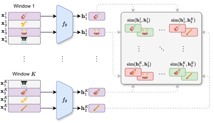
Figure 2: The COCOLA training procedure (single stem case). We first randomly crop windows of size $L$ from a batch of $K$ tracks (depicted on the left). As a second step, we randomly select two distinct stems in each window. For example, in the first window we select $\mathbf{x}^{1}_{1}$ (Guitar) and $\mathbf{x}^{1}_{3}$ (Drums). Thus, we embed all selected stems with the COCOLA encoder $f_{\theta}$, obtaining latent representations. For example, we obtain $\mathbf{h}^{1}_{1}$ and $\mathbf{h}^{1}_{2}$ from the first window. Finally, we compute the contrastive loss (Eq. (3)) considering embedings belonging to the same window as positive pairs and combinations of embeddings between different windows as negative pairs.

2 Related Work

2.1 Contrastive Methods for Audio

Contrastive learning [18, 19] can be formulated both as a supervised or self-supervised problem.

Supervised contrastive learning methods are typically cross-modal, requiring labeled information alongside audio data. In early works, the labeled information was in the form of simple tags, while the loss used to align embeddings of audio segments and tags was the triplet loss [20]. Within the same data setting,[21] used the contrastive loss of SimCLR [22]. With the advent of the transformer architecture [23], using complex sentences instead of simple tags became feasible. MuLaP [24] is the first model to train a common representation between audio and sentences in the musical domain. In such work, the audio and text are processed by a joint transformer encoder, conveying information about the two modalities through cross-attention layers. Although it is not a contrastive model per se, an audio-text matching loss uses negative examples to encourage the model to focus on aligned pairs. More recent works [25, 26, 9, 27], consider separate textual and audio encoders, which makes it possible to use the two branches independently at inference time.

Self-supervised representation learning methods [28, 29, 30, 31] build embedding spaces targeting structural information extracted from the audio data itself. In [32], the authors build positive examples for a triplet loss by augmenting with Gaussian noise, time and frequency translations, and sampling with time proximity. They also consider example mixing. While we compare coherent mixes in our method (Section 3.1), in [32], positive pairs are not coherence-related (e.g., mixing siren and dog sounds). As in the supervised case, following [22], multi-class cross-entropy losses are employed [33, 34, 35]. In COLA [33], the authors train an embedding model with contrastive loss using the simple criterion of sampling positive pairs only from the same audio track (still employing Gaussian noise), outperforming a fully supervised baseline in a plethora of tasks. [36] pairs mixtures with sources extracted via source separation.

The proposed COCOLA method shares aspects of both supervised and self-supervised approaches. Given that stems are pre-separated, we cannot consider the method purely self-supervised. At the same time, we process such data with a uni-modal encoder, as is the case of self-supervised methods.

2.2 Compositional Waveform Music Generation

Compositional music generation in the waveform domain (as opposed to symbolic domains such as MIDI or sheet music [37]) was introduced by [11], proposing the Multi-Source Diffusion Model (MSDM). Such a model captures the joint distribution of a fixed set of sources (e.g., Bass, Drums, Guitar, and Piano) using a (score-based) diffusion model [38, 39, 7, 6, 40]. At inference time, it is possible to perform unconditional generation of all sources, accompaniment generation of a subset given the complement, and source separation.

Following this initial work, AUDIT [41] proposes a diffusion model conditioned by a T5 Encoder [10], trained with instructions that allow the addition, removal (drop), and replacement of sources in an input audio mixture. This model operates on general audio signals with weak dependencies between the sources (e.g., environmental sounds). While MSDM is an unconditional generative model that processes single sources in parallel, AUDIT is a conditional generative model that processes mixtures sequentially.

InstructME [12] introduces AUDIT in the musical setting of MSDM, where sources are highly interdependent. Besides conditioning on chords, the fundamental difference lies in how the audio input is provided to the model: while in AUDIT, the input and output are two channels of the tensor that the diffusion model processes (the input is inpainted at inference time, similarly to how accompaniment generation is performed in MSDM), in InstructME, the input is processed by a convolutional network that follows the structure of the diffusion model U-Net [42] encoder. The features processed by the latter are aggregated with the features of the U-Net encoder (authors do not specify if they sum or inject the features).

StemGen [13] generates a single accompaniment source, given an instrument tag and an input audio mixture, via a masked music language model [4].

Another line of research focuses on inference-only methods for compositional music tasks, given pre-trained generative models. Based on generative source separation via Bayesian inference [43, 44, 45], Generalized Multi-Source Diffusion Inference (GMSDI) [46] performs the tasks of MSDM, requiring models trained only with mixtures and text, by separating sources while generating them.

Our proposed CompoNet baseline (Section 3.3) is a sequential conditional model that, unlike previous models, can perform all compositional music generation tasks (Figure 3). Differently than InstructME, the model is conditioned via a ControlNet adapter [17], which enables fine-tuning of diffusion models pre-trained with a large quantity of mixtures. Table 1 summarizes a comparison between CompoNet and current music compositional models.

3 Method

3.1 Stem-Level Contrastive Learning

In our setting, we have access to a dataset $D=\{\bar{\mathbf{x}}^{k}\}_{k=1,\dots,\bar{K}}$ containing $\bar{K}$ musical tracks $\bar{\mathbf{x}}^{k}$, each separated into a variable number $N$ of individual stems $\bar{\mathbf{x}}^{k}_{n}$, i.e., $\bar{\mathbf{x}}^{k}=\{\bar{\mathbf{x}}^{k}_{n}\}_{n=1,\dots,N}$. As a first step, we sample a batch of $K<\bar{K}$ tracks $\{\bar{\mathbf{x}}^{k}\}_{k=1,\dots,K}$ from $D$, with possible repetitions. Following, we slice a window $\mathbf{x}^{k}$ of size $L$ for each track $\bar{\mathbf{x}}^{k}$ in the batch (all stems in a window share the same length), such that no window contained in the same track overlaps for more than a ratio $r$, obtaining a new batch $\{\mathbf{x}^{k}\}_{k=1,\dots,K}$. Afterward, we select, for each $k$, two disjoint non-empty stem subsets $X_{1}^{k},X_{2}^{k}$ of $\mathbf{x}^{k}$. We define the sub-mixes $\mathbf{m}^{k}_{1}$ and $\mathbf{m}^{k}_{2}$ by summing the stems in $X_{1}^{k},X_{2}^{k}$:

$$\mathbf{m}^{k}_{1}=\sum_{\mathbf{x}_{n}^{k}\in X_{1}^{k}}\mathbf{x}^{k}_{n},\qquad\mathbf{m}^{k}_{2}=\sum_{\mathbf{x}_{n}^{k}\in X_{2}^{k}}\mathbf{x}^{k}_{n}$$ (1)

When $X_{1}^{k},X_{2}^{k}$ are singletons, the sub-mixes are simply two stems in the window (single stem case). We work with sub-mixes because current compositional music generation methods [13] operate over them, including our proposed CompoNet (see Section 3.3). Like in COLA[33], we use a convolutional audio-only encoder $f_{\theta}:\mathbb{R}^{L}\to\mathbb{R}^{d}$, mapping $\mathbf{m}^{k}_{1}$ and $\mathbf{m}^{k}_{2}$ to lower-dimensional embedding vectors $\mathbf{h}^{k}_{1}=f_{\theta}(\mathbf{m}^{k}_{1})$ and $\mathbf{h}^{k}_{2}=f_{\theta}(\mathbf{m}^{k}_{2})$, with $d$ the embedding dimension.

The COCOLA training procedure maximizes the agreement between pairs $\mathbf{h}^{k}_{1},\mathbf{h}^{k}_{2}$ of sub-mixes embeddings in the same window. It decreases it for pairs $\mathbf{h}^{k}_{1},\mathbf{h}^{j}_{2}$ ($j\neq k$) of sub-mixes embeddings in different windows. As in COLA, we use a bilinear similarity metric:

$$\text{sim}(\mathbf{h}^{k}_{1},\mathbf{h}^{j}_{2})=(\mathbf{h}^{k}_{1})^{T}\mathbf{W}\mathbf{h}^{j}_{2}\,,$$ (2)

where $\mathbf{W}$ is a learnable matrix. The loss we optimize is the multi-class cross entropy:

$$\mathcal{L}=-\sum^{K}_{k=1}\log\frac{\exp(\text{sim}(\mathbf{h}^{k}_{1},\mathbf{h}^{k}_{2}))}{\sum^{K}_{j=1}\exp(\text{sim}(\mathbf{h}^{k}_{1},\mathbf{h}^{j}_{2}))}\,.$$ (3)

We depict the training procedure of COCOLA in Figure 2 for the single stem case.

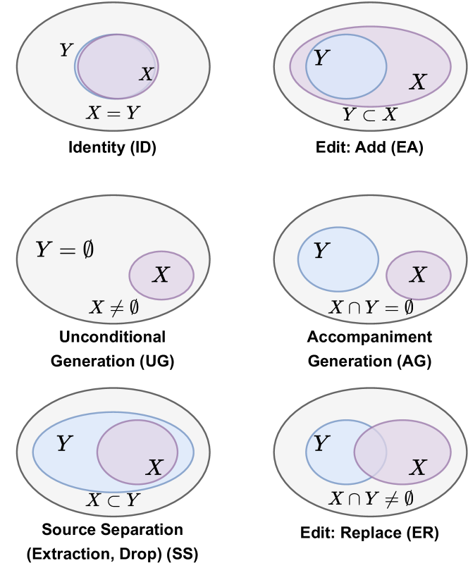
Figure 3: Inter-stem compositional generation tasks. $Y$ and $X$ represent the input and output stem sub-sets, respectively.

In the COLA training procedure, the positive pairs are (fully mixed) windows belonging to the same track. In COCOLA, they are sub-mixes belonging to the same window. As such, we allow for negative pairs belonging to the same track but in different windows. The $r$ ratio has to be chosen well to avoid strong overlaps between windows in the same track. In that case, we could potentially consider (nearly) coherent sub-mixes as negative pairs.

Model	Task					Methodology	Input	Output	Coherence
	UG	AG	SS	EA	ER
MSDM [11]	✓	✓(MS)	✓(MS)	✗	✗	Training / Supervised	Multi / Source	Multi / Source	✓
GMSDI [46]	✓	✓(MS)	✓(MS)	✗	✗	Inference / Weakly Supervised	Multi / Sub-mix	Multi / Sub-mix	✓
StemGen [13]	✓	✓(1S)	✗	✗	✗	Training / Supervised	Single / Sub-mix	Single / Source	✓
Audit [41]	✓	✗	✓(Remove 1S)	✓(1S)	✓(1S)	Training / Supervised	Single / Sub-mix	Single / Sub-mix	✗
InstructME [12]	✓	✗	✓(Extract 1S; Remove 1S)	✓(1S)	✓(1S)	Training / Supervised	Single / Sub-mix	Single / Sub-mix	✓
CompoNet	✓	✓(MS)	✓(MS)	✓(MS)	✓(MS)	Training / Supervised / Fine-tuning	Single / Sub-mix	Single / Sub-mix	✓

Table 1: Compositional audio models comparison. The various tasks are illustrated in Figure 3. 1S vs MS: the task operates on one vs multiple sources at a time. Multi vs Single on Input / Output: the model accepts multiple vs single inputs / outputs. Source vs Sub-mix on Input / Output: the model processes single sources or sub-mixes as inputs / outputs.

3.2 COCOLA Score

Equipped with the encoder $f_{\theta}$, we can quantify the coherence of the accompaniments generated by a generative model $p_{\phi}(\mathbf{x}\mid\mathbf{y})$, where $\mathbf{y}$ is the conditioning variable (the input) and $\mathbf{x}$ is the modeled variable (the output). The model’s variables can be either a set of stems or sub-mixes. Given the input $\mathbf{y}$, the model $p_{\phi}$ generates an output $\tilde{\mathbf{x}}\sim p_{\phi}(\mathbf{x}\mid\mathbf{y})$. We can compute the coherence between $\mathbf{y}$ and $\tilde{\mathbf{x}}$ by first embedding the two vectors $\mathbf{h}_{\mathbf{y}}=f_{\theta}(\mathbf{y})$ and $\mathbf{h}_{\tilde{\mathbf{x}}}=f_{\theta}(\tilde{\mathbf{x}})$ (summing the stems beforehand if considering a set of stems). We define the COCOLA score (CCS) between $\mathbf{x}$ and $\tilde{\mathbf{y}}$ as:

$$\text{CCS}(\mathbf{y},\tilde{\mathbf{x}})=\text{sim}(\mathbf{h}_{\mathbf{y}},\mathbf{h}_{\tilde{\mathbf{x}}})\,,$$ (4)

the similarity (Eq. (2)) between their embeddings. The described procedure is depicted in Figure 1.

3.3 CompoNet

In order to showcase the utility of the COCOLA score as a metric for measuring the coherence of generated accompaniments, we propose an improved compositional model for music called CompoNet and compare it with the MSDM baseline in Section 5.

CompoNet first pre-trains a latent diffusion model $\epsilon_{\phi}$, based on U-Net architecture [42] conditioned via cross-attention layers [23], on a large dataset of tuples $(\mathbf{m},\mathbf{c})$ comprising audio mixtures $\mathbf{m}$ and relative textual descriptions $\mathbf{c}$. The mixtures $\mathbf{m}$ are mapped to latent vectors $\mathbf{z}=E^{\text{VAE}}(\mathbf{m})$ using a pre-trained VAE encoder [47], while the text descriptions are mapped to a continuous sequence $\mathbf{s}=E^{\text{TXT}}(\mathbf{c})$ using a text encoder (e.g., [10]). Following the DDPM formulation [7], the model is trained to reverse the forward Gaussian noising process given by:

$$\mathbf{z}_{t}=\sqrt{\bar{\alpha}_{t}}\mathbf{z}+\sqrt{1-\bar{\alpha}_{t}}\boldsymbol{\epsilon},\quad\boldsymbol{\epsilon}\sim\mathcal{N}(\mathbf{0},\mathbf{I})\,,$$ (5)

where $t\in[0,T]$ is a time index (with $T$ the maximum time step), $\bar{\alpha}_{t}$ is defined by integrating a noise schedule [7], and $\boldsymbol{\epsilon}$ is sampled from the standard Gaussian distribution. The model is trained with denoising score matching [39]:

$$\min_{\phi}\mathbb{E}_{\mathbf{z},\boldsymbol{\epsilon},\mathbf{s},t}\left[\|\boldsymbol{\epsilon}-\epsilon_{\phi}(\mathbf{z}_{t},\mathbf{s},t)\|^{2}_{2}\right]\,,$$ (6)

with $\mathbf{z}_{t}$ obtained via Eq. (5).

In a second phase, we fine-tune a ControlNet [17] adapter $C_{\psi}$ for tackling all compositional musical tasks (Figure 3) with a single model. The U-Net $\epsilon_{\phi}$ comprises an encoder, bottleneck, decoder structure $\epsilon_{\phi}=D_{\phi_{D}}\circ B_{\phi_{B}}\circ E_{\phi_{E}}$. The ControlNet adapter is defined as $C_{\psi}(\mathbf{z}_{t},\mathbf{s},t,\mathbf{w})=E_{\phi_{E}}(\mathbf{z}_{t}+\text{conv}_{\text{in}}(\mathbf{w}),\mathbf{s},t)$, where $\text{conv}_{\text{in}}$ is a zero-initialized convolutional layer, and $\mathbf{w}$ is a latent (VAE) embedding of an external audio input. The ControlNet adapter outputs the set of processed features $\{C^{i}_{\psi}(\mathbf{z}_{t},\mathbf{s},t,\mathbf{w})\}_{i=1,\dots,I}$ for each layer of $E_{\phi_{E}}$, with $I$ the total number of layers. The full ControlNet conditional architecture is defined as $\epsilon_{\phi,\psi}=D_{\phi_{D}}\circ B_{\phi_{B}}\circ E_{\phi_{E},\psi}$ with $E_{\phi_{E},\psi}$ combining the encoder and ControlNet adapter features at each layer $i$ with zero-initialized convolutional layers $\text{conv}_{i}$:

While we have described the general ControlNet architecture, we still have to describe how we train it in CompoNet, namely, the roles of the $\mathbf{z},\mathbf{w}$ and $\mathbf{s}$ variables. Iterating over a dataset containing tuples $(\mathbf{x},\mathbf{t})$ with multi-stem tracks $\mathbf{x}=\{\mathbf{x}_{n}\}_{n=1,\dots,N}$ and tag descriptions $\mathbf{t}=\{\mathbf{t}_{n}\}_{n=1,\dots,N}$ for each stem, we sample from $\mathbf{x}$ two arbitrary subsets of stems $Y,X\subseteq\mathbf{x}$, with $|X|>0$. $Y$ contains input stems while $X$ contains output stems. The topological relationships between such subsets define all possible compositional tasks, as depicted in Figure 3. While previous models partially solve some tasks (see Table 1), ours is the first to solve all of them simultaneously. We proceed like in Eq. (1) and mix the sources in $Y$ and $X$, obtaining $\mathbf{m}_{Y}$ and $\mathbf{m}_{X}$, respectively. Afterward, we encode them in the VAE latent space, defining $\mathbf{z}=E^{\text{VAE}}(\mathbf{m}_{X})$ and $\mathbf{w}=E^{\text{VAE}}(\mathbf{m}_{Y})$. We define the following prompt $\mathbf{s}$:

$$\mathbf{s}=E^{\text{TXT}}(\mathbf{t}_{Y_{1}},\dots,\mathbf{t}_{Y_{|Y|}},\verb|SEP|,\ \mathbf{t}_{X_{1}},\dots,\mathbf{t}_{X_{|X|}})\,,$$ (7)

specifying input and output mixture tags separated by a special token SEP.

Having specified the required inputs and outputs, we train $\epsilon_{\phi,\psi}$ via Eq. (6), optimizing only the $\psi$ weights. The $\mathbf{s}$ prompt instructs the model which task to perform based on the specified stem tags. The user knows such information during the composition process in a generative DAW [48]. While we only test CompoNet on accompaniment generation against MSDM using COCOLA, we want the models to share similar abilities for a fair comparison.

4 Experimental Setup

	Test Dataset
Train Dataset	MUSDB18-HQ	MoisesDB	Slakh2100	CocoChorales
MoisesDB [49]	52.56	53.01	51.22	60.32
Slakh2100 [50]	53.06	53.58	53.78	59.35
CocoChorales [51]	70.10	61.48	67.50	99.78
All	90.43	93.06	90.06	99.89

Table 2: Classification accuracy tests (%) with COCOLA models using $K=2$ sub-mixture test pairs (higher is better). MUSDB18-HQ is used as a hold-out test dataset.

4.1 Datasets

In our experiments, we use four different stem-separated public datasets for training COCOLA and fine-tuning CompoNet. The datasets are MUSDB18-HQ [52], MoisesDB [49], Slakh2100 [50] and CocoChorales [51].

MUSDB18-HQ [52] is the uncompressed version (in WAV format) of the MUSDB18 dataset, initially introduced in [53]. This dataset is a standard for evaluating music source separation systems. It comprises 150 tracks – 100 for training and 50 for testing – totaling approximately 10 hours of professional-quality audio. Each track is divided into four stems: Bass, Drums, Vocals, and Other, with “Other” covering any components not classified under the first three categories.

MoisesDB [49] features 240 music tracks across diverse genres and artists, accumulating more than 14 hours of music. Unlike MUSDB18-HQ, MoisesDB is a genuine multi-track dataset, offering a two-tier taxonomy of 11 distinct stems. Each stem in this dataset includes more detailed type annotations (e.g., Guitar might be labeled as Acoustic Guitar or Electric Guitar). Not having pre-computed splits, we set a custom 0.8 (train) / 0.1 (validation) / 0.1 (test) split.

Slakh2100 [50] is synthesized from the Lakh MIDI Dataset v0.1 [54] employing high-quality sample-based virtual instruments. It features 2100 tracks organized into 1500 tracks for training, 375 for validation, and 225 for testing, together amounting to 145h of audio. The tracks are annotated into 34 stem categories. While such a dataset contains an order of magnitude more data than MUSDB18-HQ and MoisesDB, it does not share the same level of realism as the latter, being the tracks synthesized from MIDI.

CocoChorales [51] is a chorale audio music dataset created through a synthesis process like Slakh2100. However, it comprises a substantially vaster collection of 240000 tracks, extending over 1411 hours of audio data. It is produced by generating symbolic notes via a Coconet model, performing their synthesis with MIDI-DDSP [55]. This dataset is richly annotated, featuring details on performance attributes and synthesis parameters. CocoChorales includes a diverse range of 13 instruments spanning Strings, Brass, Woodwind, and Random ensembles. In our experiments we use the tiny version, comprising 4000 tracks.

4.2 Model Implementation

To implement the COCOLA encoder $f_{\theta}$, we follow [33] and employ the EfficientNet-B0 [56] convolutional architecture followed by a linear projection layer, operating on the mel-filterbank audio representation. The embedding dimension is 512. With respect to the original baseline, we add a $0.1$ dropout on the EfficientNet layers.

For CompoNet, we employ the AudioLDM2 [57, 58] architecture. Since the authors pre-train the model on a large array of datasets [59, 60, 61, 62, 63, 64, 65, 66], we skip the pre-training phase in Section 3.2 and directly fine-tune a ControlNet adapter based on the AudioLDM 2-Large checkpoint. During fine-tuning, we directly pass the conditioning prompt in Eq. 7 to the text-embedding mechanism of AudioLDM2 (based on CLAP [9, 27], T5 [10], and GPT2 [67]), conditioning both the U-Net and the ControlNet adapter.

Figure 4: Cosine vs bilinear similarity during training. Training is performed with “COCOLA All”. The accuracy metric is defined in Eq. (8). We adopt the bilinear similarity in Eq. (2), given its improved performance.

Method	FAD $\downarrow$ CLAP	FAD $\downarrow$ EnCodec	FAD $\downarrow$ VGGish	COCOLA score $\uparrow$ All	COCOLA score $\uparrow$ CocoChorales
Slakh2100
MSDM [11]	0.23	92.81	2.01	3.31	0.72
CompoNet	0.30	106.23	3.20	13.50	8.32
Random	0.064	51.44	0.16	0.069	1.06
Ground Truth	-	-	-	16.57	14.31
MUSDB18-HQ
MSDM [11]	0.29	148.09	2.36	11.61	3.37
CompoNet	0.37	130.04	2.14	11.94	7.21
Random	0.11	100.25	0.35	4.40	3.47
Ground Truth	-	-	-	16.25	12.45

Table 3: Comparison between MSDM and CompoNet.

4.3 Training Details

All COCOLA models are trained on an NVIDIA RTX 4070 Super with 12GB of VRAM. Each training batch contains 32 audio chunks of 5s (16kHz). We set the maximum window overlap ratio $r=50\%$ and train with the Adam optimizer [68] with a $10^{-3}$ learning rate. We add Gaussian noise to positive samples as a data augmentation method, with $\sigma=10^{-3}$. We tried training with cosine similarity [22] but we reported (Figure 4) lower performance, corroborating [33].

CompoNet models are also fine-tuned on NVIDIA GPUs (RTX 4080 16GB on MUSDB18-HQ; A10G, 24GB on Slakh2100). The training batches have size 2 (MUSDB18-HQ) and 5 (Slakh2100) and contain windows of 10.24s (16kHz). We train with Adam [68] with a $10^{-4}$ learning rate. We do not use the empty prompt for classifier-free guidance [69] during fine-tuning.

5 Experiments

We employ four COCOLA encoder models in our experiments : “COCOLA MoisesDB”, “COCOLA Slakh2100”, “COCOLA CocoChorales” and “COCOLA All”. The first three are trained on the homonym datasets, while the last one is trained on all three combined. For the “COCOLA CocoChorales” we use all ensables while on “COCOLA All” we use only the Random ensamble for a more balanced partitioning, with respect to the other datasets. MUSDB18-HQ, being the smallest dataset, is used as a held-out test dataset for studying generalization.

5.1 Coherent Sub-Mix Classification

We cross-test the performance of all COCOLA models, performing classification of coherent pairs on the test split of our datasets. More specifically, given an encoder $f_{\theta}$, we iterate a test set, collecting at each step a batch of $K$ windows $\mathbf{x}^{1},\dots,\mathbf{x}^{K}$. Following the steps in Section 3.1 we compute all similarities $\text{sim}(\mathbf{h}^{k}_{1},\mathbf{h}^{j}_{2})$ for $k,j\in[K]$. We define the accuracy over a batch as:

$$\frac{1}{K}\sum_{k=1}^{K}\mathds{1}\biggl{(}k=\operatorname*{arg\,max}_{j\in[K]}\text{sim}(\mathbf{h}^{k}_{1},\mathbf{h}^{j}_{2})\biggr{)}\,,$$ (8)

where $\mathds{1}$ is the indicator function. We obtain the final accuracy averaging over all batches in the dataset. For our evaluation we use $K=2$ and depict in Table 2 the results across all combinations of models and test datasets. While both “COCOLA MoisesDB” and “COCOLA Slakh2100” perform only slightly better than a random choice, “COCOLA CocoChorales” features improved performance. Finally, combining the three dataset, we obtain an accuracy of over 90% on all datasets, showcasing generalization with 90.43% on the held-out MUSDB18-HQ.

5.2 Accompaniment Generation Evaluation

For the accompaniment generation evaluation, we compare the MSDM model [11] with the proposed CompoNet (Section 3.3). We train CompoNet on MUSDB18-HQ and Slakh2100 (restricted to Bass, Drums, Guitar and Piano stems at test time). We also consider a Random baseline, where, for a given input, we output a random sub-mix from a different test track. We generate 200 chunks for both datasets and models, conditioning on random stem subsets of test tracks and querying a subset of the complementary. The chunks are $\sim$6s / 10.24s long on MUSDB18-HQ / Slakh2100. Given that MSDM tends to generate silence, we sample 12 candidate tracks for each generated track, selecting the one with the highest $L^{2}$ norm. We compare the COCOLA score in Eq. (4) with the FAD [16, 70] metric (interpreted as a sub-FAD [15, 11]) computed with CLAP [9], EnCodec [71], and VGGish [72] backbones.

We showcase the results in Table 3. With the FAD metrics, the model assigns the best score to the Random baseline. This behavior can be explained by considering that the Random outputs are real data, and the FAD evaluates well the perceptual quality. At the same time, it fails to assess the coherence between the tracks, and tends to score MSDM better. With the “COCOLA All” score, Random is the lowest, while CompoNet scores best. CompoNet has the highest value on “COCOLA CocoChorales” which, however, scores MSDM lower than Random. We remember that “COCOLA All” achieves a higher accuracy in Table 2, resulting in more reliability. On Ground Truth, we compute upper-bounds of the COCOLA score using real positive pairs. CompoNet better approaches these bounds.

6 Conclusion

In this paper we proposed COCOLA, a contrastive encoder for recognizing the coherence between musical stems. At the same time, we have introduced CompoNet, a novel compositional model for music based on ControlNet that can solve a wide range of tasks simultaneously. Finally, we have evaluated CompoNet using COCOLA, proposing a new way of assessing accompaniment generation.

We plan to improve the quality of COCOLA by training on additional stem-level datasets [73] or using data obtained by pre-separating [15] larger realistic music datasets [74]. In future work, we would also like to explore inference-side methods that can guide the diffusion process using COCOLA as a likelihood function, offering an alternative (or additional) loss for the GMSDI method [46].

7 Acknowledgments

The authors were partially supported by the ERC grant no. 802554 (SPECGEO), PRIN 2020 project no. 2020TA3K9N (LEGO.AI), PRIN 2022 project no. 2022AL45R2 (EYE-FI.AI, CUP H53D2300350-0001), PNRR MUR project no. PE0000013-FAIR, and AWS Cloud Credit for Research program.

References

- [1] A. Agostinelli, T. I. Denk, Z. Borsos, J. Engel, M. Verzetti, A. Caillon, Q. Huang, A. Jansen, A. Roberts, M. Tagliasacchi et al., “Musiclm: Generating music from text,” arXiv preprint arXiv:2301.11325, 2023.
- [2] J. Copet, F. Kreuk, I. Gat, T. Remez, D. Kant, G. Synnaeve, Y. Adi, and A. Défossez, “Simple and controllable music generation,” Advances in Neural Information Processing Systems, vol. 36, 2024.
- [3] F. Schneider, Z. Jin, and B. Schölkopf, “Moûsai: Text-to-music generation with long-context latent diffusion,” arXiv preprint arXiv:2301.11757, 2023.
- [4] H. F. Garcia, P. Seetharaman, R. Kumar, and B. Pardo, “Vampnet: Music generation via masked acoustic token modeling,” arXiv preprint arXiv:2307.04686, 2023.
- [5] Z. Evans, C. Carr, J. Taylor, S. H. Hawley, and J. Pons, “Fast timing-conditioned latent audio diffusion,” arXiv preprint arXiv:2402.04825, 2024.
- [6] Y. Song, J. Sohl-Dickstein, D. P. Kingma, A. Kumar, S. Ermon, and B. Poole, “Score-based generative modeling through stochastic differential equations,” in International Conference on Learning Representations, 2021. [Online]. Available: https://openreview.net/forum?id=PxTIG12RRHS
- [7] J. Ho, A. Jain, and P. Abbeel, “Denoising diffusion probabilistic models,” in Proceedings of the 34th International Conference on Neural Information Processing Systems, 2020, pp. 6840–6851.
- [8] OpenAI, “Gpt-4 technical report,” 2023.
- [9] B. Elizalde, S. Deshmukh, M. Al Ismail, and H. Wang, “Clap learning audio concepts from natural language supervision,” in ICASSP 2023-2023 IEEE International Conference on Acoustics, Speech and Signal Processing (ICASSP). IEEE, 2023, pp. 1–5.
- [10] C. Raffel, N. Shazeer, A. Roberts, K. Lee, S. Narang, M. Matena, Y. Zhou, W. Li, and P. J. Liu, “Exploring the limits of transfer learning with a unified text-to-text transformer,” Journal of machine learning research, vol. 21, no. 140, pp. 1–67, 2020.
- [11] G. Mariani, I. Tallini, E. Postolache, M. Mancusi, L. Cosmo, and E. Rodolà, “Multi-source diffusion models for simultaneous music generation and separation,” in The Twelfth International Conference on Learning Representations, 2024.
- [12] B. Han, J. Dai, X. Song, W. Hao, X. He, D. Guo, J. Chen, Y. Wang, and Y. Qian, “Instructme: An instruction guided music edit and remix framework with latent diffusion models,” arXiv preprint arXiv:2308.14360, 2023.
- [13] J. D. Parker, J. Spijkervet, K. Kosta, F. Yesiler, B. Kuznetsov, J.-C. Wang, M. Avent, J. Chen, and D. Le, “Stemgen: A music generation model that listens,” in ICASSP 2024-2024 IEEE International Conference on Acoustics, Speech and Signal Processing (ICASSP). IEEE, 2024, pp. 1116–1120.
- [14] M. Grachten, S. Lattner, and E. Deruty, “Bassnet: A variational gated autoencoder for conditional generation of bass guitar tracks with learned interactive control,” Applied Sciences, vol. 10, no. 18, 2020. [Online]. Available: https://www.mdpi.com/2076-3417/10/18/6627
- [15] C. Donahue, A. Caillon, A. Roberts, E. Manilow, P. Esling, A. Agostinelli, M. Verzetti, I. Simon, O. Pietquin, N. Zeghidour et al., “Singsong: Generating musical accompaniments from singing,” arXiv preprint arXiv:2301.12662, 2023. [Online]. Available: https://arxiv.org/abs/2301.12662
- [16] D. Roblek, K. Kilgour, M. Sharifi, and M. Zuluaga, “Fr’echet audio distance: A reference-free metric for evaluating music enhancement algorithms,” in Proc. Interspeech, 2019, pp. 2350–2354.
- [17] L. Zhang, A. Rao, and M. Agrawala, “Adding conditional control to text-to-image diffusion models,” in Proceedings of the IEEE/CVF International Conference on Computer Vision, 2023, pp. 3836–3847.
- [18] S. Chopra, R. Hadsell, and Y. LeCun, “Learning a similarity metric discriminatively, with application to face verification,” in 2005 IEEE Computer Society Conference on Computer Vision and Pattern Recognition (CVPR’05), vol. 1, 2005, pp. 539–546 vol. 1.
- [19] A. v. d. Oord, Y. Li, and O. Vinyals, “Representation learning with contrastive predictive coding,” arXiv preprint arXiv:1807.03748, 2018.
- [20] F. Schroff, D. Kalenichenko, and J. Philbin, “Facenet: A unified embedding for face recognition and clustering,” in Proceedings of the IEEE conference on computer vision and pattern recognition, 2015, pp. 815–823.
- [21] X. Favory, K. Drossos, T. Virtanen, and X. Serra, “COALA: Co-aligned autoencoders for learning semantically enriched audio representations,” in ICML 2020 Workshop on Self-supervision in Audio and Speech, 2020. [Online]. Available: https://openreview.net/forum?id=7jxwhNDM0Uv
- [22] T. Chen, S. Kornblith, M. Norouzi, and G. Hinton, “A simple framework for contrastive learning of visual representations,” in International conference on machine learning. PMLR, 2020, pp. 1597–1607.
- [23] A. Vaswani, N. Shazeer, N. Parmar, J. Uszkoreit, L. Jones, A. N. Gomez, Ł. Kaiser, and I. Polosukhin, “Attention is all you need,” Advances in neural information processing systems, vol. 30, 2017.
- [24] I. Manco, E. Benetos, E. Quinton, and G. Fazekas, “Learning music audio representations via weak language supervision,” in ICASSP 2022-2022 IEEE International Conference on Acoustics, Speech and Signal Processing (ICASSP). IEEE, 2022, pp. 456–460.
- [25] ——, “Contrastive audio-language learning for music,” in Ismir 2022 Hybrid Conference, 2022.
- [26] Q. Huang, A. Jansen, J. Lee, R. Ganti, J. Y. Li, and D. P. Ellis, “Mulan: A joint embedding of music audio and natural language,” in Ismir 2022 Hybrid Conference, 2022.
- [27] Y. Wu, K. Chen, T. Zhang, Y. Hui, T. Berg-Kirkpatrick, and S. Dubnov, “Large-scale contrastive language-audio pretraining with feature fusion and keyword-to-caption augmentation,” in ICASSP 2023-2023 IEEE International Conference on Acoustics, Speech and Signal Processing (ICASSP). IEEE, 2023, pp. 1–5.
- [28] S. Pascual, M. Ravanelli, J. Serrà, A. Bonafonte, and Y. Bengio, “Learning problem-agnostic speech representations from multiple self-supervised tasks,” Interspeech 2019, 2019.
- [29] M. Tagliasacchi, B. Gfeller, F. d. C. Quitry, and D. Roblek, “Pre-training audio representations with self-supervision,” IEEE Signal Processing Letters, vol. 27, pp. 600–604, 2020.
- [30] H.-H. Wu, C.-C. Kao, Q. Tang, M. Sun, B. McFee, J. P. Bello, and C. Wang, “Multi-task self-supervised pre-training for music classification,” in ICASSP 2021-2021 IEEE International Conference on Acoustics, Speech and Signal Processing (ICASSP). IEEE, 2021, pp. 556–560.
- [31] P.-Y. Huang, H. Xu, J. Li, A. Baevski, M. Auli, W. Galuba, F. Metze, and C. Feichtenhofer, “Masked autoencoders that listen,” Advances in Neural Information Processing Systems, vol. 35, pp. 28 708–28 720, 2022.
- [32] A. Jansen, M. Plakal, R. Pandya, D. P. Ellis, S. Hershey, J. Liu, R. C. Moore, and R. A. Saurous, “Unsupervised learning of semantic audio representations,” in 2018 IEEE international conference on acoustics, speech and signal processing (ICASSP). IEEE, 2018, pp. 126–130.
- [33] A. Saeed, D. Grangier, and N. Zeghidour, “Contrastive learning of general-purpose audio representations,” in ICASSP 2021-2021 IEEE International Conference on Acoustics, Speech and Signal Processing (ICASSP). IEEE, 2021, pp. 3875–3879.
- [34] H. Al-Tahan and Y. Mohsenzadeh, “Clar: Contrastive learning of auditory representations,” in International Conference on Artificial Intelligence and Statistics. PMLR, 2021, pp. 2530–2538.
- [35] J. Spijkervet, J. Burgoyne et al., “Contrastive learning of musical representations.” ISMIR, 2021.
- [36] C. Garoufis, A. Zlatintsi, and P. Maragos, “Multi-source contrastive learning from musical audio,” arXiv preprint arXiv:2302.07077, 2023.
- [37] R. Yuan, H. Lin, Y. Wang, Z. Tian, S. Wu, T. Shen, G. Zhang, Y. Wu, C. Liu, Z. Zhou et al., “Chatmusician: Understanding and generating music intrinsically with llm,” arXiv preprint arXiv:2402.16153, 2024.
- [38] J. Sohl-Dickstein, E. A. Weiss, N. Maheswaranathan, and S. Ganguli, “Deep unsupervised learning using nonequilibrium thermodynamics,” in Proceedings ICML 2015, Lille, France, 6-11 July 2015, ser. JMLR Workshop and Conference Proceedings, F. R. Bach and D. M. Blei, Eds., vol. 37. JMLR.org, 2015, pp. 2256–2265. [Online]. Available: http://proceedings.mlr.press/v37/sohl-dickstein15.html
- [39] Y. Song and S. Ermon, “Generative modeling by estimating gradients of the data distribution,” in Advances in Neural Information Processing Systems 32: Annual Conference on Neural Information Processing Systems 2019, NeurIPS 2019, December 8-14, 2019, Vancouver, BC, Canada, H. M. Wallach, H. Larochelle, A. Beygelzimer, F. d’Alché-Buc, E. B. Fox, and R. Garnett, Eds., 2019, pp. 11 895–11 907.
- [40] T. Karras, M. Aittala, T. Aila, and S. Laine, “Elucidating the design space of diffusion-based generative models,” in Advances in Neural Information Processing Systems, 2022. [Online]. Available: https://openreview.net/forum?id=k7FuTOWMOc7
- [41] Y. Wang, Z. Ju, X. Tan, L. He, Z. Wu, J. Bian et al., “Audit: Audio editing by following instructions with latent diffusion models,” Advances in Neural Information Processing Systems, vol. 36, 2024.
- [42] O. Ronneberger, P. Fischer, and T. Brox, “U-net: Convolutional networks for biomedical image segmentation,” in Medical Image Computing and Computer-Assisted Intervention–MICCAI 2015: 18th International Conference, Munich, Germany, October 5-9, 2015, Proceedings, Part III 18. Springer, 2015, pp. 234–241.
- [43] V. Jayaram and J. Thickstun, “Source separation with deep generative priors,” in International Conference on Machine Learning. PMLR, 2020, pp. 4724–4735.
- [44] G. Zhu, J. Darefsky, F. Jiang, A. Selitskiy, and Z. Duan, “Music source separation with generative flow,” IEEE Signal Processing Letters, vol. 29, pp. 2288–2292, 2022.
- [45] E. Postolache, G. Mariani, M. Mancusi, A. Santilli, L. Cosmo, and E. Rodolà, “Latent autoregressive source separation,” in Proceedings of the AAAI Conference on Artificial Intelligence, vol. 37, no. 8, 2023, pp. 9444–9452.
- [46] E. Postolache, G. Mariani, L. Cosmo, E. Benetos, and E. Rodolà, “Generalized multi-source inference for text conditioned music diffusion models,” in ICASSP 2024 - 2024 IEEE International Conference on Acoustics, Speech and Signal Processing (ICASSP), 2024, pp. 6980–6984.
- [47] D. P. Kingma and M. Welling, “Auto-encoding variational bayes,” in 2nd International Conference on Learning Representations, ICLR 2014, Banff, AB, Canada, April 14-16, 2014, Conference Track Proceedings, Y. Bengio and Y. LeCun, Eds., 2014.
- [48] I. Clester and J. Freeman, “Composing with generative systems in the digital audio workstation 145-148,” in Joint Proceedings of the IUI 2023 Workshops: HAI-GEN, ITAH, MILC, SHAI, SketchRec, SOCIALIZE co-located with the ACM International Conference on Intelligent User Interfaces (IUI 2023), Sydney, Australia, March 27-31, 2023, ser. CEUR Workshop Proceedings, A. Smith-Renner and P. Taele, Eds., vol. 3359. CEUR-WS.org, 2023, pp. 145–148. [Online]. Available: https://ceur-ws.org/Vol-3359/paper15.pdf
- [49] I. G. Pereira, F. Araujo, F. Korzeniowski, and R. Vogl, “Moisesdb: A dataset for source separation beyond 4 stems,” in Ismir 2023 Hybrid Conference, 2023.
- [50] E. Manilow, G. Wichern, P. Seetharaman, and J. Le Roux, “Cutting music source separation some Slakh: A dataset to study the impact of training data quality and quantity,” in Proc. IEEE Workshop on Applications of Signal Processing to Audio and Acoustics (WASPAA). IEEE, 2019, pp. 45–49.
- [51] Y. Wu, J. Gardner, E. Manilow, I. Simon, C. Hawthorne, and J. Engel, “The chamber ensemble generator: Limitless high-quality mir data via generative modeling,” arXiv preprint arXiv:2209.14458, 2022.
- [52] Z. Rafii, A. Liutkus, F.-R. Stöter, S. I. Mimilakis, and R. Bittner, “Musdb18-hq - an uncompressed version of musdb18,” Aug. 2019. [Online]. Available: https://doi.org/10.5281/zenodo.3338373
- [53] Z. Rafii, A. Liutkus, F.-R. Stöter, S. I. Mimilakis, and R. Bittner, “The MUSDB18 corpus for music separation,” Dec. 2017. [Online]. Available: https://doi.org/10.5281/zenodo.1117372
- [54] C. Raffel, “Learning-based methods for comparing sequences, with applications to audio-to-midi alignment and matching,” Ph.D. dissertation, Columbia University, USA, 2016. [Online]. Available: https://doi.org/10.7916/D8N58MHV
- [55] Y. Wu, E. Manilow, Y. Deng, R. Swavely, K. Kastner, T. Cooijmans, A. Courville, C.-Z. A. Huang, and J. Engel, “Midi-ddsp: Detailed control of musical performance via hierarchical modeling,” in International Conference on Learning Representations, 2021.
- [56] M. Tan and Q. Le, “Efficientnet: Rethinking model scaling for convolutional neural networks,” in International conference on machine learning. PMLR, 2019, pp. 6105–6114.
- [57] H. Liu, Z. Chen, Y. Yuan, X. Mei, X. Liu, D. Mandic, W. Wang, and M. D. Plumbley, “Audioldm: text-to-audio generation with latent diffusion models,” in Proceedings of the 40th International Conference on Machine Learning, 2023, pp. 21 450–21 474.
- [58] H. Liu, Q. Tian, Y. Yuan, X. Liu, X. Mei, Q. Kong, Y. Wang, W. Wang, Y. Wang, and M. D. Plumbley, “Audioldm 2: Learning holistic audio generation with self-supervised pretraining,” arXiv preprint arXiv:2308.05734, 2023.
- [59] J. F. Gemmeke, D. P. W. Ellis, D. Freedman, A. Jansen, W. Lawrence, R. C. Moore, M. Plakal, and M. Ritter, “Audio set: An ontology and human-labeled dataset for audio events,” in 2017 IEEE International Conference on Acoustics, Speech and Signal Processing (ICASSP), 2017, pp. 776–780.
- [60] X. Mei, C. Meng, H. Liu, Q. Kong, T. Ko, C. Zhao, M. D. Plumbley, Y. Zou, and W. Wang, “Wavcaps: A chatgpt-assisted weakly-labelled audio captioning dataset for audio-language multimodal research,” arXiv preprint arXiv:2303.17395, 2023.
- [61] C. D. Kim, B. Kim, H. Lee, and G. Kim, “AudioCaps: Generating captions for audios in the wild,” in Proceedings of the 2019 Conference of the North American Chapter of the Association for Computational Linguistics: Human Language Technologies, Volume 1 (Long and Short Papers), J. Burstein, C. Doran, and T. Solorio, Eds. Minneapolis, Minnesota: Association for Computational Linguistics, Jun. 2019, pp. 119–132. [Online]. Available: https://aclanthology.org/N19-1011
- [62] H. Chen, W. Xie, A. Vedaldi, and A. Zisserman, “Vggsound: A large-scale audio-visual dataset,” in ICASSP 2020-2020 IEEE International Conference on Acoustics, Speech and Signal Processing (ICASSP). IEEE, 2020, pp. 721–725.
- [63] M. Defferrard, K. Benzi, P. Vandergheynst, and X. Bresson, “Fma: A dataset for music analysis,” in International Society for Music Information Retrieval Conference, 2016.
- [64] T. Bertin-Mahieux, D. P. Ellis, B. Whitman, and P. Lamere, “The million song dataset,” in Proceedings of the 12th International Conference on Music Information Retrieval (ISMIR 2011), 2011.
- [65] G. Chen, S. Chai, G. Wang, J. Du, W.-Q. Zhang, C. Weng, D. Su, D. Povey, J. Trmal, J. Zhang et al., “Gigaspeech: An evolving, multi-domain asr corpus with 10,000 hours of transcribed audio,” arXiv preprint arXiv:2106.06909, 2021.
- [66] K. Ito and L. Johnson, “The lj speech dataset,” https://keithito.com/LJ-Speech-Dataset/, 2017.
- [67] T. Brown, B. Mann, N. Ryder, M. Subbiah, J. D. Kaplan, P. Dhariwal, A. Neelakantan, P. Shyam, G. Sastry, A. Askell et al., “Language models are few-shot learners,” Advances in neural information processing systems, vol. 33, pp. 1877–1901, 2020.
- [68] D. Kingma and J. Ba, “Adam: A method for stochastic optimization,” in International Conference on Learning Representations (ICLR), San Diega, CA, USA, 2015.
- [69] J. Ho and T. Salimans, “Classifier-free diffusion guidance,” in NeurIPS 2021 Workshop on Deep Generative Models and Downstream Applications, 2021.
- [70] A. Gui, H. Gamper, S. Braun, and D. Emmanouilidou, “Adapting frechet audio distance for generative music evaluation,” in ICASSP 2024-2024 IEEE International Conference on Acoustics, Speech and Signal Processing (ICASSP). IEEE, 2024, pp. 1331–1335.
- [71] A. Défossez, J. Copet, G. Synnaeve, and Y. Adi, “High fidelity neural audio compression,” Transactions on Machine Learning Research, 2023. [Online]. Available: https://openreview.net/forum?id=ivCd8z8zR2
- [72] S. Hershey, S. Chaudhuri, D. P. Ellis, J. F. Gemmeke, A. Jansen, R. C. Moore, M. Plakal, D. Platt, R. A. Saurous, B. Seybold et al., “Cnn architectures for large-scale audio classification,” in 2017 IEEE International Conference on Acoustics, Speech and Signal Processing (ICASSP). IEEE, 2017.
- [73] S. Sarkar, E. Benetos, and M. Sandler, “Ensembleset: a new high quality synthesised dataset for chamber ensemble separation,” in Ismir 2022 Hybrid Conference, 2022.
- [74] D. Bogdanov, M. Won, P. Tovstogan, A. Porter, and X. Serra, “The mtg-jamendo dataset for automatic music tagging,” in Machine Learning for Music Discovery Workshop, International Conference on Machine Learning (ICML 2019), Long Beach, CA, United States, 2019. [Online]. Available: http://hdl.handle.net/10230/42015