A Closer Look at Classification Evaluation Metrics and a Critical Reflection of Common Evaluation Practice

Abstract

Classification systems are evaluated in a countless number of papers. However, we find that evaluation practice is often nebulous. Frequently, metrics are selected without arguments, and blurry terminology invites misconceptions. For instance, many works use so-called ‘macro’ metrics to rank systems (e.g., ‘macro F1’) but do not clearly specify what they would expect from such a ‘macro’ metric. This is problematic, since picking a metric can affect paper findings as well as shared task rankings, and thus any clarity in the process should be maximized.

Starting from the intuitive concepts of bias and prevalence, we perform an analysis of common evaluation metrics, considering expectations as found expressed in papers. Equipped with a thorough understanding of the metrics, we survey metric selection in recent shared tasks of Natural Language Processing. The results show that metric choices are often not supported with convincing arguments, an issue that can make any ranking seem arbitrary. This work aims at providing overview and guidance for more informed and transparent metric selection, fostering meaningful evaluation.

1 Introduction

Classification evaluation is ubiquitous: we have a system that predicts some classes of interest (aka classifier) and want to assess its prediction skill. We study a widespread and seemingly clear-cut setup of multi-class evaluation, where we compare a classifier’s predictions against reference labels in two steps. First, we construct a confusion matrix that has a designated dimension for each possible prediction/label combination. Second, an aggregate statistic, which we denote as metric, summarizes the confusion matrix as a single number.

Already from this it would follow that ‘the perfect’ metric can’t exist, since important information is bound to get lost when reducing the confusion matrix to a single dimension. Still, we require a metric to rank and select classifiers, and thus it should characterize a classifier’s ‘skill’ or ‘performance’ as well as possible. But exactly what is a ‘performance’ and how should we measure it? Such questions do not seem to arise (as much) in other ‘performance’ measurements that are known to humans. E.g., a marathon’s result derives from a clear and broadly accepted criterion (time over distance) that can be measured with validated instruments (a clock). However, in machine learning, criterion and instrument are often less clear and lie entangled in the term ‘metric’.

metric	cited motivation/argument
macro F1	“macro-averaging (…) implies that all class
	labels have equal weight in the final score”
macro P/R/F1	“because (…) skewed distribution
	of the label set”
macro F1	“Given the strong imbalance between the
	number of instances in the different classes”
Accuracy, macro F1	“the labels are imbalanced”
MCC	“balanced measurement when the classes
	are of very different sizes”
MCC, F1	“(…) imbalanced data (…)”
macro F1	“(…) imbalanced classes (…) introduce
	biases on accuracy”
macro F1	“due to the imbalanced dataset”

Table 1: Typical comments that intend to motivate metric selection. MCC: Matthews Correlation Coefficient.

Since metric selection can influence which system we consider better or worse in a task, one would think that metrics are selected with great care. But when searching through papers for reasons that would support a particular metric choice, we mostly (at best) find only weak or indirect arguments. E.g., it is observed (Table 1) that ‘labels are imbalanced’ or it is wished for that ‘all class labels have equal weight’. These perceived problems or needs are then often supposedly addressed with a ‘macro’ metric (Table 1).

However, what is meant with phrases like ‘imbalanced data’ or ‘macro’ is rarely made explicit, and how the metrics that are then selected in this context are actually addressing a perceived ‘imbalance’ is unclear. According to a word etymology, evaluation with a ‘macro’ metric may involve the expectation that we are told a bigger picture of classifier capability (Greek: makrós, ‘long/large’), whereas a smaller picture (Greek: mikrós, ‘small’) would perhaps bind the assessment to a more local context. Regardless of such musings, it is clear that blurry terminology in the context of classifier evaluation can lead to results that may be misconceived by readers and authors alike.

This paper aims to serve as a handy reference for anyone who wishes to better understand classification evaluation, how evaluation metrics align with expectations expressed in papers, and how we might construct an individual case for (or against) selecting a particular evaluation metric.

Paper outline.

After introducing Preliminaries (§2) and five Metric Properties (§3), we conduct a thorough Metric Analysis (§4) of common classification measures: ‘Accuracy’ (§4.1), ‘Macro Recall and Precision’ (§4.2, §4.3), two different ‘Macro F1’ (§4.4, §4.5), ‘Weighted F1’ (§4.6), as well as ‘Kappa’ and ‘Matthews Correlation Coefficient (MCC)’ in §4.7. We then show how to create simple but meaningful Metric Variants (§5). We wrap up the theoretical part with a Discussion (§6) that includes a short Summary (§6.1) of our main analysis results in Table 5. Next we study Metric Selection in Shared Tasks (§7) and give Recommendations (§8). Finally, we contextualize our work against some Background and Related Work (§9), and finish with Conclusions (§10).

2 Preliminaries

We introduce a set of intuitive concepts as a basis.

Classifier, confusion matrix, and metric.

For any classifier $f:D\rightarrow C=\{1,...,n\}$ and finite set $S\subseteq D\times C$, let $m^{f,S}\in\mathbb{R}_{\geq 0}^{n\times n}$ be a confusion matrix where $m^{f,S}_{ij}=|\{s\in S~{}|~{}f(s_{1})=i\land s_{2}=j\}|$. We omit superscripts whenever possible. So generally, $m_{i,j}$ contains the mass of events where the classifier predicts $i$, and the true label is $j$. That is, on the diagonal of the matrix lies the mass of correct predictions, and all other fields indicate the mass of specific errors. A $metric:\mathbb{R}_{\geq 0}^{n\times n}\rightarrow(-\infty,1]$ then allows us to order confusion matrices, respectively, rank classifiers (bounds are chosen for convenience). We say that (for a data set $S$) a classifier $f$ is better than (or preferable to) a classifier $g$ iff $metric(m^{f,S})>metric(m^{g,S})$, i.e., a higher score indicates a better classifier.

Let us now define five basic quantities:

Class bias, prevalence and correct

are given as

$$bias(i)=\sum_{x}m_{i,x}~{}~{}~{}~{}~{}~{}prevalence(i)=\sum_{x}m_{x,i}$$

$$correct(i)=m_{i,i}.~{}~{}~{}~{}~{}~{}~{}~{}~{}~{}~{}~{}~{}~{}~{}~{}~{}~{}~{}~{}~{}~{}~{}~{}~{}$$

Class precision.

$P_{i}$ is the precision for class $i$:

$$P_{i}=\frac{correct(i)}{bias(i)}\approx\mathcal{P}(c=i|f\rightarrow i).$$ (1)

It approximates the probability of observing a correct class given a specific prediction.

Class recall.

$R_{i}$ denotes the recall for class $i$,

$$R_{i}=\frac{correct(i)}{prevalence(i)}\approx\mathcal{P}(f\rightarrow i|c=i),$$ (2)

that approximates the probability of observing a correct prediction given an input of a certain class.

3 Defining metric properties

To understand and distinguish metrics in more precise ways, we define five metric properties: Monotonicity, class sensitivity, class decomposability, prevalence invariance and chance correction.

3.1 Monotonicity (PI)

Take a classifier that receives an input. If the prediction is correct, we would naturally expect that the evaluation score does not decrease, and if it is wrong, the evaluation score should not increase. We cast this clear expectation into

Property I (Monotonicity).

A $metric$ has PI iff:

$$\forall m:\frac{\partial metric(m)}{\partial m_{i,j}}\begin{cases}\geq 0\impliedby i=j\\ \leq 0\impliedby i\neq j,\end{cases}$$ (3)

i.e., diagonal fields of the confusion matrix (correct mass) should yield a non-negative ‘gradient’ in the metric, while for all other fields (containing error mass) it should be non-positive. PI assumes differentiability of a metric, but it can be simply extended to the discrete case.

3.2 Macro metrics are class-sensitive (PII)

A ‘macro’ metric needs to be sensitive to classes, or else it could not yield a ‘balanced measurement’ for ‘classes having different sizes’ (c.f. Table 1). By contrast, a ‘micro’ metric should care only about whether predictions are wrong or right, which would bind its score more to a local context of a specific data set and its class distribution. This means for macro metrics that they should possess

Property II (Class sensitivity).

PII is given iff $\exists m\in\mathbb{R}_{\geq 0}^{|C|\times|C|}$ with $\frac{\partial metric(m)}{\partial m_{i,i}}\neq\frac{\partial metric(m)}{\partial m_{j,j}}$, $(i,j)\in C^{2}$ or $\frac{\partial metric(m)}{\partial m_{i,j}}\neq\frac{\partial metric(m)}{\partial m_{k,l}}$, $(i,j,k,l)\in C^{4},i\neq j,k\neq l$.

A metric without PII is not a macro metric.

3.3 Macro average: Mean over classes (PIII)

‘Macro’ metrics are sometimes named ‘macro-average’ metrics. This suggests that they may be perceived as an average over classes. We introduce

Property III (Class decomposability).

A ‘macro-average’ metric can be stated as

$$metric(m)^{g}_{p}=\left(\frac{1}{n}\sum_{i=1}^{n}g(m_{i},(m^{T})_{i},i)^{p}\right)^{\frac{1}{p}},$$ (4)

i.e., as an unweighted mean over class-specific scores from inputs examples related to a specific class ($c=i$ $\lor$ $f\rightarrow i$). E.g., later we will see that ‘macro F1’ is a specific parameterization of Eq. 4.

3.4 Strictly “Treat all classes equally” (PIV)

A common argument for using metrics other than the ratio of correct predictions is that we want to ‘not neglect rare classes’ and ‘show classifier performance equally [w.r.t.] all classes’.

Nicely, with the assumption of class prevalence being the only important difference across data sets, we could then even say that classifier $f$ is generally better than (or preferable to) $g$ iff $metric(m^{f})>metric(m^{g})$, further disentangling a classifier comparison from a specific data set. At first glance, PIII seems to capture this wish already, by virtue of an unweighted mean over classes. However, the score w.r.t. one class is still influenced by the prevalence of other classes, and thus the result of the mean can change in non-transparent ways if class frequency is varied.

		$c=$
		x	y
	x	15	5
$f$$\rightarrow$	y	10	10

Table 2: Class $y$ occurs 15 times.

		$c=$
		x	y
	x	15 $\cdot 1$	5 $\cdot 2$
$f$$\rightarrow$	y	10 $\cdot 1$	10 $\cdot 2$

Table 3: Apply $\mathbb{\lambda}=(1,2)$.

		$c=$
		x	y
	x	15	10
$f$$\rightarrow$	y	10	20

Table 4: Class $y$ occurs 30 times.

Therefore it makes sense to define such an expectation (‘treat all classes equally’) more strictly. We simulate different class prevalences with a

Prevalence scaling.

We can use a diagonal prevalence scaling matrix $\mathbb{\lambda}$ to set

$$m^{\prime}=m\mathbb{\lambda}.$$ (5)

By scaling a column $i$ with $\lambda_{ii}$, we inflate (or deflate) the mass of data that belong to class $i$ (e.g., see Tables 4, 4, 4), but retain the relative proportions of intra-class error types. Now, we can define

Property IV (Prevalence invariance).

If $(\mathbb{\lambda},\mathbb{\lambda}^{\prime})\in\mathbb{R}_{>0}^{n\times n}\times\mathbb{R}_{>0}^{n\times n}$ is a pair of diagonal matrices then $metric(m\mathbb{\lambda})=metric(m\mathbb{\lambda}^{\prime})$.

Prevalence calibration.

There is a special case of $\lambda$. We select $\lambda^{\sim}$ s.t. all classes have the same prevalence. We call this prevalence calibration:

$$\lambda_{ii}^{\sim}=\frac{|S|}{n\cdot prevalence(i)}.$$ (6)

3.5 Chance correction (PV)

Two simple ‘baseline’ classifiers are: Predicting classes uniformly randomly, or based on observed prevalence. A macro metric can be expected to show robustness against any such chance classifier and be chance corrected, assigning a clear and comparable baseline score. Thus, it should have

Property V (Chance Correction).

A $metric$ has PV iff for any (large) dataset $S$ with $n$ classes and set $A$ with arbitrary random classifiers:

$$\max\big{\{}metric(m^{r,S})~{}~{}|~{}~{}r\in A\big{\}}=\omega(n^{S})<<1.$$

Here, $\omega$ returns an upper-bound baseline score from the number of classes $n^{S}$ alone. If it also holds that $\max\{...\}=\min\{...\}=\omega(n^{S})$, we say that $metric$ is strictly chance corrected, and in the case where $\forall S,r:~{}metric(m^{r,S})=\Omega~{}\text{(constant)}$ we speak of complete chance correction.

Less formally, chance correction means that the metric score attached to any chance baseline has a bound that is known to us (the bound generalizes over data sets but not over the number of classes). Strict chance correction means additionally that any chance classifier’s score will be the same, and just depends on the number of classes. Finally, complete chance correction means that every chance classifier always yields the same score, regardless of the number of classes. Note that strictness or completeness may not always be desired, since they can marginalize empirical overall correctness in a data set. Any chance correction, however, increases the evaluation interpretability by contextualizing the evaluation with an interpretable baseline score.

4 Metric property analysis

Equipped with the appropriate tools, we are now ready to start the analysis of classification metrics. We will study ‘Accuracy’, ‘Macro Recall’, ‘Macro Precision’, ‘Macro F1’, ‘Weighted F1’, ‘Kappa’, and ‘Matthews Correlation Coefficient’ (MCC).

4.1 Accuracy (aka Micro F1)

Accuracy is the ratio of correct predictions:

$$accuracy=\frac{\sum_{i}m_{i,i}}{\sum_{(i,j)}m_{i,j}}=\frac{1}{|S|}\sum_{i}correct(i).$$

Property analysis.

As a ‘micro’ metric, Accuracy has only PI (monotonicity). This is expected, since PII-V aim at macro metrics. Interestingly, in multi-class evaluation, $accuracy$ equals ‘micro Precion, micro Recall and micro F1’ that sometimes occur in papers. See Appendix A for proofs.

Discussion.

Accuracy is an important statistic, estimating the probability of observing a correct prediction in a data set. But this means that it is strictly tied to the class prevalences in a specific data set. And so, in the pursuit of some balance or a more generalizable score, researchers seem interested in other metrics.

4.2 Macro Recall: ticks five boxes

Macro Recall is defined as the unweighted arithmetic mean over all class-wise recall scores:

$$macR=\frac{1}{n}\sum_{i}R_{i}=\frac{1}{n}\sum_{i}\frac{correct(i)}{prevalence(i)}.$$ (7)

Property analysis.

Macro Recall has all five properties (Proofs in Appendix B). It is also strictly chance corrected with $\omega(n)=1/n$.

Discussion.

Since macro Recall has all five properties, including prevalence invariance (PIV), it may be a good pick for evaluation, particularly through a ‘macro’ lens. It also offers three intuitive interpretations: Drawing an item from a random class, Bookmaker metric and prevalence-calibrated Accuracy.

In the first interpretation, we draw a random item from a randomly selected class. What’s the probability that it is correctly predicted? $MacR$ estimates the answer $\sum_{i}\frac{1}{n}\cdot\mathcal{P}(f\rightarrow i|c=i)$.

Alternatively, we wear the lens of a (fair) Bookmaker. For every prediction (bet), we pay 1 coin and gain coins per fair (European) odds. The odds for making a correct bet, when the class is $i$, are $odds(i)=\frac{|S|}{prevalence(i)}$. So for each data example $(x,y)$, our bet is evaluated ($\mathbb{I}[f(x)=y]\in\{0,1\}$), and thus we incur a total net

$$win =\sum_{s\in S}\bigg{(}\mathbb{I}[f(s_{1})=s_{2}]\cdot odds(s_{2})-1\bigg{)}$$

$$=\sum_{s\in S}\bigg{(}\mathbb{I}[f(s_{1})=s_{2}]\cdot odds(s_{2})\bigg{)}-|S|$$

$$=\sum_{i=1}^{n}\bigg{[}odds(i)\cdot\sum_{\begin{subarray}{c}s\in S\\ s_{2}=i\end{subarray}}\bigg{(}\mathbb{I}[f(s_{1})=i]\bigg{)}\bigg{]}-|S|$$

$$=|S|\sum_{i=1}^{n}\frac{correct(i)}{prevalence(i)}-|S|$$

$$=n|S|\cdot macR-|S|=|S|(n\cdot macR-1),$$

which is positive only if $macR>1/n$.

Finally we can view macro Recall as Accuracy after prevalence calibration. Set $\lambda$ as in Eq. 6:

$$macAcc =accuracy(m\lambda^{\sim})$$

$$=\frac{\sum_{i}{\lambda_{ii}^{\sim}\cdot correct(i)}}{\sum_{i}{\lambda_{ii}^{\sim}\cdot prevalence(i)}}$$ (8)

$$=\sum_{i}R_{i}/\sum_{i}1=macR.$$

4.3 Macro Precision: is the bias an issue?

Macro Precision is the unweighted arithmetic mean over class-wise precision scores:

$$macP=\frac{1}{n}\sum_{i}P_{i}=\frac{1}{n}\sum_{i}\frac{correct(i)}{bias(i)}.$$ (9)

Property analysis.

While properties I, II, III, V are fulfilled, macro Precision does not have prevalence invariance (Proofs in Appendix C). With some $\lambda$, the max. score difference ($macP(m)$ vs. $macP(m\lambda)$) approaches $1-\frac{1}{n}$. Like macro Recall, it is strictly chance corrected ($\omega(n)=1/n$).

Discussion.

Macro Precision wants to approximate the probability to see a correct prediction, given we randomly draw one out of $n$ different predictions. Hence, $macP$ seems to provide us with an interesting measure of ‘prediction trustworthiness’. An issue is that the score does not generalize across different class prevalences, since $bias(i)\propto\mathcal{P}(f\rightarrow i)=\sum_{j}\mathcal{P}(f\rightarrow i,c=j)$ is subject to change if prevalences of other classes $j\neq i$ vary ($\propto$ means approximately proportional to). Therefore, even though $macP$ is decomposed over classes (PIII), it is not invariant to prevalence changes (PIV), and if we have $f,f^{\prime}$ with different biases, score differences are difficult to interpret, particularly with an underlying ‘macro’ expectation that a metric be robust to class prevalence.

To mitigate the issue, we can use prevalence calibration (Eq. 6), yielding

$$correct^{\sim}(i)=\lambda_{i,i}^{\sim}m_{i,i}\propto\mathcal{P}(f\rightarrow i|c=i),$$

$$bias^{\sim}(i)=\sum_{j}\lambda_{j,j}^{\sim}m_{i,j}\propto\sum_{j}\mathcal{P}(f\rightarrow i|c=j),$$

and a $macP^{\sim}$ that has been updated with a prior belief that all classes have the same prevalence. Like macro Recall, $macP^{\sim}$ is now detached from the class distribution in a specific data set, treating all classes more literally ‘equally’.

4.4 Macro F1: Metric of choice in many tasks

Macro F1 is often used for evaluation. It is commonly defined as an arithmetic mean over class-wise harmonic means of precision and recall:

$$macF1 =\frac{1}{n}\sum_{i}F1_{i}=\frac{1}{n}\sum_{i}\frac{2P_{i}R_{i}}{P_{i}+R_{i}}$$ (10)

$$=\frac{2}{n}\sum_{i}\frac{correct(i)}{bias(i)+prevalence(i)}.$$

Property analysis.

Again, all properties except PIV are fulfilled (Proofs in Appendix D). Interestingly, while macro F1 has PV (chance correction), the chance correction isn’t strict, differentiating it from other macro metrics: Indeed, its chance baseline upper bound $\omega(n)=1/n$ is achieved only if $\mathcal{P}(f\rightarrow i)=\mathcal{P}(c=i)$, meaning that macro F1 not only corrects for chance, but also factors in more data set accuracy (like a ‘micro’ score). Additionally, the second line of the formula shows that macro F1 is invariant to the false-positive and false-negative error spread for a specific class.

Discussion.

Macro F1 wants the distribution of prediction and class prevalence to be similar (a micro feature), but also high correctness for every class, by virtue of the unweighted mean over classes (a macro feature). Thus it seems useful to find classifiers that do well in a given data set, but probably also in others, a ‘balance’ that could explain its popularity. However, macro F1 inherits an interpretability issue of Precision. It doesn’t strictly ‘treat all classes equally’ as per PIV, at least not without prevalence calibration (Eq. 6).

4.5 Macro F1: A doppelganger

Interestingly, there is another metric that has been coined ‘macro F1’. We find a first(?) mention in Sokolova and Lapalme (2009) and evaluation usage (made explicit) in a lot of papers, i.a., Stab and Gurevych (2017); Mohammadi et al. (2020); Rodrigues and Branco (2022). This macro F1 is the harmonic mean of macro Precision and Recall:

$$macF1^{\prime}=\frac{2\cdot macR\cdot macP}{macR+macP}.$$ (11)

Property analysis.

In contrast to its name twin, one less property is given (PIII), since it cannot be decomposed over classes (Proofs in Appendix E), and it is strictly chance corrected with $\omega(n)=1/n$. Opitz and Burst (2019) prove that Eq. 11 and Eq. 10 can diverge to a large degree of up to 0.5.

Discussion.

Putting the harmonic mean on the outside, and the arithmetic means on the inside, $macF1^{\prime}$ seems to stick a tad more true to the emphasis in its name (F1, aka harmonic mean). However, $macF1^{\prime}$ does not seem as easy to interpret, since the numerator involves the cross-product of all class-wise recall and precision values. We might view it through the lens of an inter-annotator agreement (IAA) metric though, treating classifier and reference as two annotators:

$$macF1^{\prime}=\frac{2\cdot macR(m)\cdot macR(m^{T})}{macR(m)+macR(m^{T})},$$ (12)

falling back on $macR$’s clear interpretation(s).

4.6 Weighted F1

‘Weighted F1’ or ‘Weighted average F1’ is yet another F1 variant that has been used for evaluation:

$$weightF1=\frac{1}{|S|}\sum_{i}prevalence(i)\cdot F1_{i}.$$

Property analysis.

Weighted F1 is sensible to classes (PII). The other four properties are not featured, which means that it is also non-monotonic. See Appendix F for proofs.

Discussion.

While measuring performance ‘locally’ for each class, the results are weighted by class-prevalence. Imagining metrics on a spectrum from ‘micro’ to ‘macro’, $weightF1$ sits next to Accuracy, the prototypical micro metric. This is also made obvious by its featured properties, where only one would mark a ‘macro’ metric (PII). Due to its lowered interpretability and non-monotonicity, we may wonder why $weightF1$ would be preferred over Accuracy. Finally, with prevalence calibration, it reduces to macro F1, $weightF1(m\lambda^{\sim})=macF1(m\lambda^{\sim})$, similar to how calibrated Accuracy reduces to macro Recall.

4.7 Birds of a feather: Kappa and MCC

Assuming normalized confusion matrices, we can state both metrics as concise as possible. Let $\mathbf{1}$ be a vector with ones of dimension $n$. Then let

$$\mathbf{b}=m\mathbf{1};\text{~{}~{}}\mathbf{p}=m^{T}\mathbf{1};\text{~{}~{}}chance=\mathbf{p}^{T}\mathbf{b}.$$ (13)

I.e., at index $i$ of vector $\mathbf{p}$, we find $prevalence(i)$, and at index $i$ of vector $\mathbf{b}$ we find $bias(i)$.

Generalized Matthews correlation coefficient (MCC).

The multi-class generalization of MCC Gorodkin (2004) can now be written concisely as

$$MCC=\frac{accuracy-chance}{(\sqrt{1-\mathbf{b}^{T}\mathbf{b}})(\sqrt{1-\mathbf{p}^{T}\mathbf{p}})}.$$ (14)

Cohen’s kappa

Cohen (1960) is then denoted as follows, illuminating its similarity to MCC:

$$KAPPA=\frac{accuracy-chance}{1-chance}.$$ (15)

Property analysis.

MCC and Kappa have PII and PV (complete chance correction: $\Omega=0$). However, they are non-monotonic (PI), not class-decomposable (PIII), and not prevalence-invariant (PIV); Proofs in Appendix G. Further note that $sgn(MCC)=sgn(KAPPA)$ and $|MCC|\geq|KAPPA|$, since $\mathbf{p}^{T}\mathbf{b}\leq\{\mathbf{b}^{T}\mathbf{b},\mathbf{p}^{T}\mathbf{p}\}$.

Discussion.

Kappa and MCC are similar measures. Since $chance\approx\sum_{i}\mathcal{P}(c=i)\cdot\mathcal{P}(f\rightarrow i)$ allows the interpretation of observing a prediction that is correct just by chance, Kappa and MCC can be viewed as a standardized Accuracy.

However, overall they are standardized in slightly different ways. The denominator of Kappa simply shows the upper bound, i.e., the perfect classifier, which is intuitive. How do we interpret $\mathbf{b}^{T}\mathbf{b}$ and $\mathbf{p}^{T}\mathbf{p}$ in MCC? Given two random items drawn from two random classes, $\mathbf{b}^{T}\mathbf{b}$ seems to measure the chance that the classifier randomly predicts the same label, while $\mathbf{p}^{T}\mathbf{p}$ measures the chance that the true labels are the same. This adds complexity to the MCC formula that can make classifier comparison less clear. The stronger dependence on classifier bias through $\mathbf{b}^{T}\mathbf{b}$ also favors classifiers with uneven biases, regardless of the actual class distribution in a data set. This reduced interpretability is still evident when the measures are prevalence-calibrated (Eq. 6):

$$KAPPA(m\lambda^{\sim})=\frac{macR-1/n}{1-1/n}$$ (16)

$$MCC(m\lambda^{\sim})=\frac{macR-1/n}{(\sqrt{1-\mathbf{b^{\sim}}^{T}\mathbf{b^{\sim}}})(\sqrt{1-1/n})},$$

which reduces KAPPA (but not MCC) to $macR$.

metric	PI (mono.)	PII (class sens.)	PIII (decomp.)	PIV (prev. invar.)	PV (chance correct.)
Accuracy (=Micro F1)	✓	✗${}_{\text{({\color[rgb]{0,0,0}\char 51})}}$	✗${}_{\text{({\color[rgb]{0,0,0}\char 51})}}$	✗${}_{\text{({\color[rgb]{0,0,0}\char 51})}}$	✗${}_{\text{({\color[rgb]{0,0,0}\char 51})}}$
macro Recall ($macR$)	✓	✓	✓	✓	✓: $1/n$, strict
as $GmacR$ or $HmacR$	✓	✓	✓	✓	✓: $1/n$
macro Precision	✓	✓	✓	✗${}_{\text{({\color[rgb]{0,0,0}\char 51})}}$	✓: $1/n$, strict
macro F1 ($macF1$)	✓	✓	✓	✗${}_{\text{({\color[rgb]{0,0,0}\char 51})}}$	✓: $1/n$
macro F1’ ($macF1^{\prime}$)	✓	✓	✗	✗${}_{\text{({\color[rgb]{0,0,0}\char 51})}}$	✓: $1/n$, strict
weighted F1	✗	✓	✗${}_{\text{({\color[rgb]{0,0,0}\char 51})}}$	✗${}_{\text{({\color[rgb]{0,0,0}\char 51})}}$	✗${}_{\text{({\color[rgb]{0,0,0}\char 51})}}$
Kappa	✗	✓	✗	✗${}_{\text{({\color[rgb]{0,0,0}\char 51})}}$	✓: 0, complete
MCC	✗	✓	✗	✗${}_{\text{({\color[rgb]{0,0,0}\char 51})}}$	✓: 0, complete

Table 5: Summary of evaluation metric properties. ✗${}_{\text{({\color[rgb]{0,0,0}\char 51})}}$: a property is fulfilled after prevalence calibration.

5 Metric variants

5.1 Mean parameterization in PIII

It is interesting to consider $p\neq 1$ in the generalized mean (Eq. 4). E.g., in the example of macro Recall, setting $p\rightarrow 0$ yields the geometric mean

$$GmacR=GM(R_{1},...,R_{n})=\sqrt[n]{R_{1}\cdot...\cdot R_{n}}.$$

Same as $macR$, it has all five properties. Given $n$ random items, one from every class, $GmacR$ approximates a (class-count normalized) probability that all are correctly predicted. Hence, $GmacR$ can be useful when it’s important to perform well in all classes. Thinking further along this line, we can employ $HmacR$ ($p=-1$) with the harmonic mean $HM(R_{1},...,R_{n})=n(\frac{1}{R_{1}}+...+\frac{1}{R_{n}})^{-1}$.

5.2 Prevalence calibration

Property PIV (prevalence invariance) is rare, but we saw that it can be artificially enforced. Indeed, if we standardize the confusion matrix by making sure every class has the same prevalence (Eq. 5, Eq. 6), we ensure prevalence invariance (PIV) for a measure. As an effect of this, we found that Kappa and Accuracy reduce to macro Recall, and weighted F1 becomes the same as macro F1. For a more detailed interpretation of prevalence calibration, see our discussion for macro Precision (§4.3).

When does a prevalence calibration make sense? Since prevalence calibration offers a gain in ‘macro’-features, it can be used with the aim to push a metric more towards a ‘macro’ metric.

6 Discussion

6.1 Summary of metric analyses

Table 5 shows an overview of the visited metrics. We make some observations: i) macro Recall has all five properties, including class prevalence invariance (PIV), i.e., ‘it treats all classes equally’ (in a strict sense). However, through prevalence calibration, all metrics obtain PIV. ii) Kappa, MCC, and weighted F1 do not have property PI. Under some circumstances, errors can increase the score, possibly lowering interpretability. iii) All metrics except Accuracy and weighted F1 show chance baseline correction. Strict chance baseline correction isn’t a feature of Macro F1, and complete (class-count independent) chance correction is only achieved with MCC and Kappa.

Macro Recall and Accuracy seem to complement each other. Both have a clear interpretation, and relate to each other with a simple prevalence calibration. Indeed, macro Recall can be understood as a prevalence-calibrated version of Accuracy. On the other hand, macro F1 is interesting since it does not strictly correct for chance (as in macro Recall) but also factors in more of the test set correctness (as in a ‘micro’ score).

MCC and Kappa are similar measures, where Kappa tends to be slightly more interpretable and shows more robustness to classifier biases. Somewhat also similar are Accuracy and weighted F1, both are greatly affected by class-prevalence. As discussed in §4.6, we could not determine clear reasons for favoring weighted F1 over Accuracy.

6.2 What are other ‘balances’?

The concept of ‘balance’ seems positively flavored, and thus we may wish to reflect on more ‘balances’ other than prevalence invariance (PIV).

Another type of ‘balance’ is introduced by $GmacR$ (or $HmacR$). By virtue of the geometric (harmonic) mean that puts more weight on low outliers, they favor a classifier that equally distributes its correctness over classes. This is also reflected by $macR$ being strictly chance corrected with $1/n$, while its siblings have $1/n$ as the upper bound only achieved by the uniform random baseline, and the metrics’ gradients that scale with low-recall outliers (Appendix B.5, B.6).

Yet again another type of ‘balance’ we saw in macro F1 ($macF1$) that selects a classifier with high recall over many classes (as featured by a ‘macro’ metric) and maximizes empirical data set correctness (as featured by a ‘micro’ metric), an attribute that is also visible in its chance baseline upper bound ($1/n$) that is only achieved by a prevalence-informed baseline.

Finally, a ‘meta balance’ could be achieved when we are unsure which metric to use, by ensembling a score from a set of selected metrics.

6.3 Value of class-wise Recall

Interestingly, from class-wise recall scores we can guess the precision scores in another data set (in the absence of a reference). First, we state an estimate of the class distribution $P(c)\approx\widehat{P(c)}$ that can be expected. Then we estimate $P(f)\approx\widehat{P(f)}$, simply by running the classifier. Finally, the precision for a class $i$ will then equal

$$\frac{P(f\rightarrow i|c=i)\cdot{P(c=i)}}{P(f\rightarrow i)}\approx\frac{R_{i}\cdot\savestack{\tmpbox}{\stretchto{\scaleto{\scalerel*[\widthof{P(c=i)}]{\kern-0.6pt\bigwedge\kern-0.6pt}{\rule[-702.78297pt]{4.30554pt}{702.78297pt}}}{}}{0.5ex}}\stackon[1pt]{P(c=i)}{\tmpbox}}{\savestack{\tmpbox}{\stretchto{\scaleto{\scalerel*[\widthof{P(f\rightarrow i)}]{\kern-0.6pt\bigwedge\kern-0.6pt}{\rule[-702.78297pt]{4.30554pt}{702.78297pt}}}{}}{0.5ex}}\stackon[1pt]{P(f\rightarrow i)}{\tmpbox}}.$$

Estimated scores of macro metrics follow. It is not possible to project new recall values from old precision scores (since these do not transfer), underlining the value of recall statistics. Note that this is an idealized approximation, and complex phenomena such as domain shifts are (same as in other parts of this work) not at all accounted for.

			standard													after prevalence calibration
sys	off. r	citations	Acc	macR	macP	macF1	macF1’	weightF1	Kappa	MCC	GmacR	HmacR	r1	r2	r3	macF1	macF1’	Kappa	MCC
A	1	555	65.1	68.1	65.5	65.4	66.8	64.5	46.5	48.0	66.8	65.4	82.9	51.2	70.2	67.7	68.2	52.1	52.6
B	1	271	65.8	68.1	67.4	66.0	67.8	65.1	47.3	49.2	66.5	65.0	87.8	51.4	65.2	67.7	68.7	52.2	53.1
C	3	20	66.1	67.6	66.2	66.0	66.9	65.7	47.2	48.1	66.8	66.0	81.7	56.0	65.2	67.5	68.0	51.4	51.8
D	4	12	65.2	67.4	64.9	65.1	66.1	64.8	46.3	47.3	66.5	65.6	80.3	54.2	67.6	67.1	67.5	51.0	51.3
E	5	23	66.4	66.9	65.4	66.0	66.1	66.4	47.0	47.0	66.8	66.8	69.8	64.0	66.8	67.3	67.5	50.3	50.5
F	6	11	64.8	65.9	63.9	64.5	64.9	64.7	45.0	45.4	65.6	65.4	73.5	58.7	65.6	66.1	66.3	48.9	49.0
G	7	2	63.3	64.9	63.6	63.4	64.2	63.1	43.0	43.8	64.2	63.5	77.4	53.9	63.5	64.9	65.4	47.4	47.7
H	8	30	64.3	64.5	63.1	63.7	63.8	64.4	43.6	43.6	64.5	64.5	65.3	63.6	64.5	64.9	65.2	46.7	47.0

Table 6: Shared task ranking. ‘off. r’ is the official rank of a system. r$i$: recall for class $i$.

7 Reflecting on SemEval shared tasks

So far, we had focused on theory. Now we want to take a look at applied evaluation practice. We study works from the SemEval series, a large annual NLP event where teams compete in various tasks, many of which are classification tasks.

7.1 Example shared task study

As an example, we first study the popular SemEval shared task Rosenthal et al. (2017) on tweet sentiment classification (positive/negative/neutral) with team predictions thankfully made available.

Insight: Different metric $\rightarrow$ different ranking.

In Table 6 we see the results of the eight best of 37 systems. The two ‘winning’ systems (A, B, Table 6) were determined with $macR$, which is legitimate. Yet, system E also does quite well: it obtains highest Accuracy, and it achieves a better balance over the three classes ($R_{1}=69.8,R_{2}=64.0,R_{3}=66.8$, max. $\Delta=5.8$) as opposed to, e.g., system B ($R_{1}=87.8,R_{2}=51.4$, $R_{3}=65.2$ max. $\Delta=36.4$), indicated, on average, also by $GmacR$ and $HmacR$ metrics. So if we want to ensure performance under high uncertainty of class prevalence (as expected in Twitter data?), we may prefer system E, a system that would be also ranked higher when using an ensemble of metrics.

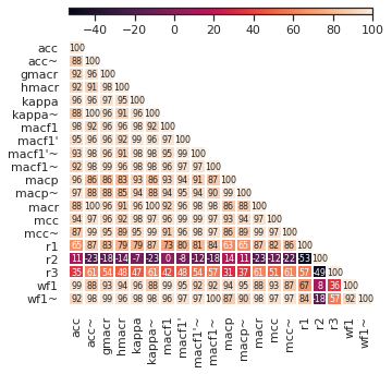
Figure 1: Team ranking correlation matrix wrt. metrics. metric~  means that the confusion matrix has been calibrated before metric computation (Eq. 6).

Figure 1 shows a pair-wise Spearman $\rho$ correlation of team rankings of all 37 teams according to different metrics. There are only 4 pairs of metrics that are in complete agreement ($\rho=100$): Macro Recall agrees with calibrated Kappa and calibrated Accuracy. This makes sense: As we before (Eq. 4.2, Eq. 16), they are equivalent (the same applies to weighted F1 and macro F1, after calibration). Looking at single classes, it seems that the second class is the one that can tip the scale: $R_{2}$ disagrees in its team ranking with all other metrics ($\rho\leq 14$).

Do rankings impact paper popularity?

For the eight best systems in Table 6, we retrieve their citation count from Google scholar as a (very coarse) proxy for their popularity. The result invites the speculation that a superficial ordering could already be effectual: While both team 1 (A) and team 2 (B) were explicitly selected as the winner of the shared task, the first-listed system appears to have almost double the amount of citations (even though B performs better as per most metrics). The citations of other systems (C–H) do not exceed lower double digits, although we saw that a case can even be made for E (rank 6) that achieves stable performance over all classes.

7.2 Examining metric argumentation

Our selected example task used macro Recall for winner selection. While the measure had been selected with care (its value became also evident in our analysis), we saw that systems were very close and arguments could have been made for selecting a slightly different (set of) winner(s). To our surprise, in a large proportion of shared tasks, the situation seems worse. Annotating 42 classification shared task overview papers from the recent 5 years, we find that

• only 23.8% papers provide a formula, and

• only 10.9% provide a sensible argument for their metric. 14.3% use a weak argument similar to the ones shown in Table 1. A large amount (73.8%) does not state an argument or employ a ‘trope’ like “As is standard, …”.

The most frequent metric in our sample is ‘macro F1’ ($macF1$). In some cases, its doppelganger $macF1^{\prime}$ seems to have been used, or a ‘balanced Accuracy’. Sometimes, in the absence of further description or formula, it can be hard to tell which ‘macro F1’ metric has been used, also due to deviating naming (macro-average F1, mean F1, macro F1, etc.). In at least one case, this has led to a disadvantage: Fang et al. (2023) report that “During model training and validation, we were not aware that the challenge organizers used a different method for calculating macro F1, namely by using the averages of precision and recall”, a measure that is much different (cf. §4.4).

We also may wonder about the situation beyond SemEval. While a precise characterization of a broader picture would escape the scope of this paper, a cursory glance shows the observed unclarities in research papers from all kinds of domains.

8 Recommendations

Overall, we would like to refrain from making bold statements as to which metric is ‘better’, since different contexts may easily call for different metrics. Still, from our analyses, we can synthesize some general recommendations:

• State the evaluation metric clearly, best use a formula. This also helps protect against ambiguity, e.g., as induced through homonyms such as $macF1$ and $macF1^{\prime}$.

• Try building a case for a metric: As a starting point we can think about how the class distribution in our data set would align with the distribution that we could expect in an application. With greater uncertainty, more macro metric features may be useful. For finer selection, consider viewing our analyses, checking any desirable metric features. Our summary (§6.1) can provide guidance.

• Consider presenting more than a single number. In particular, complementary metrics such as Accuracy and macro Recall can be indicative about i) a classifier’s empirical data set correctness (as in a micro metric) and ii) its robustness to class distribution shifts (as in a macro metric). If the amount of classes $n$ is low, consider presenting class-wise recall scores for their generalizability. If $n$ is larger and a metric is decomposable over classes (PIII), reporting the variance of a ‘macro’ metric over classes can also be of value.

• Consider admitting multiple ‘winners’ or ‘best systems’: If we are not able to build a strong case for a single metric, then it may be sensible to present a set of well-motivated metrics and select a set of best systems. If one ‘best’ system needs be selected, an average over such a set could be a useful heuristic.

9 Background and related work

Meta studies of classification metrics.

Surveys or dedicated book chapters can provide a useful introduction to classification evaluation Sokolova and Lapalme (2009); Manning (2009); Tharwat (2020); Grandini et al. (2020). Deeper analysis has been provided mostly in the two-class setting: In a series of articles by David MW Powers, we find the (previously mentioned) Bookmaker’s perspective on metrics Powers (2011), a critique of the F1 Powers (2015) and Kappa Powers (2012). Delgado and Tibau (2019) study binary MCC and Kappa (favoring MCC), while Sebastiani (2015) defines axioms for binary evaluation, including a monotonicity axiom akin to a stricter version of our PI, advocating a ‘K-metric’. Luque et al. (2019) analyze binary confusion matrices, and Chicco and Jurman (2020) compare F1, Accuracy and MCC, concluding that “MCC should be preferred (…) by all scientific communities”. The mathematical relationship between the two macro F1s is further analyzed by Opitz and Burst (2019).

Overall, we want to advocate for a mostly agnostic stance as to what metric might be picked in a case (if it is sensibly done so), remembering our premise from the introduction: the perfect metric doesn’t exist. Thus, we aimed at balancing intuitive interpretation and analysis of metrics, while acknowledging desiderata as worded in papers.

Other classification evaluation methods

can be required when class labels reside on a nominal ‘Likert’ scale O’Neill (2017); Amigo et al. (2020), or in a hierarchy Kosmopoulos et al. (2015), or they are ambiguous and need be matched (e.g., ‘none’/‘null’/‘other’) across annotation styles Fu et al. (2020), or their number is unknown Ge et al. (2017). Classifiers are also evaluated with P-R curves Flach and Kull (2015) or a receiver-operator characteristic Fawcett (2006); Honovich et al. (2022). The CheckList Ribeiro et al. (2020) proposes behavioral testing of classifiers, and the NEATCLasS workshop series Ross et al. (2023) is an effort to find novel ways of evaluation.

10 Conclusion

Starting from a definition of the two basic and intuitive concepts of classifier bias and class prevalence, we examined common classification evaluation metrics, resolving unclear expectations such as those that pursue a ‘balance’ through ‘macro’ metrics. Our metric analysis framework, including definitions and properties, can aid in the study of other or new metrics. A main goal of our work is to provide guidance for more informed decision making in metric selection.

Appendix A Accuracy aka micro Precision/Recall/F1

Micro F1 is defined as the harmonic mean ($HM$) of ‘micro Precision’ and ‘micro Recall’, where micro Precision and micro Recall are

$$\frac{\sum_{x}correct(x)}{\sum_{x}bias(x)}~{}~{}\text{and}~{}~{}\frac{\sum_{x}correct(x)}{\sum_{x}prevalence(x)}.$$

Now it suffices to see that $\sum_{x}prevalence(x)=\sum_{x}bias(x)$ and $HM(a,a)=a$.

A.1 Monotonicity $\checkmark$

$i$$\neq$$j$: $\frac{\partial Acc(m)}{\partial m_{i,j}}=-\frac{\sum_{k}correct(k)}{|S|^{2}}=-\frac{Acc}{|S|}\leq 0$; else $\frac{\partial Acc(m)}{\partial m_{i,i}}=\frac{|S|-\sum_{k}correct(k)}{|S|^{2}}=\frac{1-Acc}{|S|}\geq 0$.

A.2 Other properties

It is easy to see that properties other than Monotonicity are not featured by Accuracy.

Appendix B Macro Recall

B.1 Monotonicity ✓

If $i\neq j$: $\frac{\partial macR(m)}{\partial m_{i,j}}=-\frac{correct(j)}{n\cdot prevalence(j)^{2}}\leq 0$; else $\frac{\partial macR(m)}{\partial m_{i,i}}=\frac{prevalence(i)-correct(i)}{n\cdot prevalence(i)^{2}}\geq 0.$

B.2 Class sensitivity ✓

Follows from above.

B.3 Class decomposability ✓

In Eq. 4 set $g(row,col,x)=\frac{row_{x}}{\sum_{i}col_{i}}$ and $p=1$.

B.4 Prevalence invariance ✓

$R^{\prime}_{i}=\frac{\lambda_{i,i}m_{i,i}}{\sum_{j}\lambda_{i,i}m_{j,i}}=\frac{\lambda_{i,i}m_{i,i}}{\lambda_{i,i}\sum_{j}m_{j,i}}=R_{i}$.

B.5 Chance correction ✓

Assume normalized class prevalences $p\in[0,1]^{n}~{}\text{s.t.}~{}\sum_{i=1}^{n}p_{i}=1$ and arbitrary random baseline $z\in[0,1]^{n}~{}\text{s.t.}~{}\sum_{i=1}^{n}z_{i}=1$:

$$MacR =\frac{1}{n}\sum_{i}R_{i}=\frac{1}{n}\sum_{i}\frac{p_{i}\cdot z_{i}}{p_{i}}=\frac{1}{n},$$

$$GmacR =\sqrt[n]{\prod_{i=1}^{n}z_{i}}\leq\frac{1}{n},$$

$$HmacR =\frac{n}{\sum_{i=1}^{n}\frac{1}{z_{i}}}\leq\frac{n}{\sum_{i=1}^{n}n}=\frac{1}{n}.$$

We see that all macro Recall variants are chance corrected. $macR$ is strictly chance corrected.

B.6 Gradients for $GmacR$ and $HmacR$

For comparison we also include $macR$ with arithmetic mean ($AM$). Let $\mu_{x}=(n\cdot prevalence(x))^{-1}$, then ($i,j$ implies $i\neq j$):

$$\frac{\partial AM}{\partial m_{i,i}}=\mu_{i}(1-R_{i});~{}~{}~{}~{}~{}~{}~{}~{}~{}~{}~{}~{}~{}\frac{\partial AM}{\partial m_{i,j}}=-\mu_{j}R_{j};$$

$$\frac{\partial GM}{\partial m_{i,i}}=GM\mu_{i}(R_{i}^{-1}-1);~{}~{}\frac{\partial GM}{\partial m_{i,j}}=-GM\mu_{j};$$

$$\frac{\partial HM}{\partial m_{i,i}}=HM^{2}\mu_{i}(R_{i}^{-2}-R_{i}^{-1});$$

$$\frac{\partial HM}{\partial m_{i,j}}=-HM^{2}\mu_{j}R_{j}^{-1}.~{}~{}~{}~{}~{}~{}~{}~{}~{}~{}~{}~{}$$

Appendix C Macro Precision

C.1 Monotonicity ✓

If $i\neq j$: $\frac{\partial macP(m)}{\partial m_{i,j}}=-\frac{correct(i)}{n\cdot bias(i)^{2}}\leq 0$; else $\frac{\partial macP(m)}{\partial m_{i,i}}=\frac{bias(i)-correct(i)}{n\cdot bias(i)^{2}}\geq 0$.

C.2 Class sensitivity ✓

Follows from above.

C.3 Class decomposability ✓

In Eq. 4 set $g(row,col,x)=\frac{row_{x}}{\sum_{i}row_{i}}$ and $p=1$.

C.4 Prevalence invariance

A counter-example $P^{\prime}_{i}=\frac{\lambda_{i,i}m_{i,i}}{\sum_{j}\lambda_{j,j}m_{i,j}}\neq P_{i}$ is easily found. E.g., in Table 4, 4, 4: $macP=0.5\frac{3}{4}+0.5\frac{1}{2}=\frac{5}{8}\neq macP^{\prime}=0.5\frac{3}{5}+0.5\frac{2}{3}=\frac{19}{30}$.

C.5 Chance correction ✓

Given same assumptions as in B.5 we have

$$\frac{1}{n}\sum_{i}P_{i}=\frac{1}{n}\sum_{i}\frac{p_{i}\cdot z_{i}}{\sum_{j}z_{i}\cdot p_{j}}=\frac{1}{n}\sum_{i}p_{i}=\frac{1}{n}.$$

Appendix D Macro F1

D.1 Monotonicity ✓

Let $Z_{x}=bias(x)+prevalence(x)$. If $i\neq j$:

$$\frac{\partial macF1(m)}{\partial m_{i,j}}=-\frac{2correct(i)}{nZ_{i}^{2}}-\frac{2correct(j)}{nZ_{j}^{2}}\leq 0$$

else:

$$\frac{\partial macF1(m)}{\partial m_{i,i}} =\frac{2}{nZ_{i}}-\frac{2\cdot correct(i)}{nZ_{i}^{2}}\geq 0.$$

D.2 Class sensitivity ✓

Follows from above.

D.3 Class decomposability ✓

In Eq. 4 set $p=1$, $g(row,col,x)=\frac{2row_{x}}{\sum_{i}row_{i}+col_{i}}$.

D.4 Prevalence invariance

It is not prevalence-invariant, c.f. C.4.

D.5 Chance correction ✓

Given same assumptions as in B.5 we have

$$MacF1 =\frac{1}{n}\sum_{i}\frac{2\cdot p_{i}\cdot z_{i}}{\sum_{j}z_{i}\cdot p_{j}+\sum_{j}z_{j}\cdot p_{i}}$$ (17)

$$=\frac{1}{n}\sum_{i}\frac{2\cdot p_{i}\cdot z_{i}}{p_{i}+z_{i}}.$$ (18)

We see that a maximum is attained when p = z, and that this maximum is $\frac{1}{n}$.

Appendix E Macro F1 (name twin)

E.1 Monotonicity ✓

Let $(macR+macP-macP\cdot macR)=\epsilon\geq 0$. We have $\frac{\partial macF1^{\prime}(m)}{\partial m_{i,j}}=\frac{2x\epsilon}{macR+macP}$ where $x=(\frac{\partial macR(m)}{\partial m_{i,j}}+\frac{\partial macP(m)}{\partial m_{i,j}})$. Since $macR$ and $macP$ are monotonic, $macF1^{\prime}$ also has monotonicity.

E.2 Label sensitivity ✓

Follows from above.

E.3 Class decomposability

Not possible.

E.4 Prevalence invariance

It is not prevalence-invariant, c.f. C.4.

E.5 Chance correction ✓

Since $macF1^{\prime}$ is the $HM$ of(strictly chance corrected) macro Precision and macro Recall, we also have strictly chance correction with $\frac{1}{n}$.

Appendix F Weighted F1

F.1 Monotonicity

For brevity, let $prevalence(i)$, $bias(i)$, $correct(i)$ $=$ $x_{i}$, $y_{i}$, $z_{i}$. If $i\neq j$:

$$\frac{\partial weightF1(m)}{\partial m_{i,j}}=$$

$$\frac{1}{|S|}\bigg{(}\frac{2y_{j}z_{j}}{(x_{j}+y_{j})^{2}}-\frac{2x_{i}z_{i}}{(x_{i}+y_{i})^{2}}-weightF1\bigg{)}\overset{\text{\large\lightning}}{\leq}0.$$

If we fix the positive term, and let the others approach zero, then is a situation, where $weightF1$ increases even though a classifier made an error.

F.2 Label sensitivity ✓

Follows from above.

F.3 Class decomposability

Not possible.

F.4 Prevalence invariance

Trivial.

F.5 Chance correction

Trivial.

Appendix G Kappa and MCC

G.1 Monotonicity

We resort back to Kappa and MCC formulas for non-normalized confusion matrices, multiplying numerator and denominator by $s^{2}$, where $s=\sum_{(i,j)}m_{i,j}$ is the number of data examples, and write $r$ for $\sum_{i}{correct(i)}$.

Kappa.

We have

$$KAPPA=\frac{rs-\mathbf{p^{T}b}}{s^{2}-\mathbf{p^{T}b}}=\frac{N_{K}}{D_{K}}.$$ (19)

Other variables were introduced before (Eq. 13). Now, let $z_{ij}=prevalence(i)+bias(j)$.

Then, iff $i\neq j$:

$$\frac{\partial KAPPA}{\partial m_{i,j}}=\frac{(r-z_{ij})D_{K}^{2}-(2s-z_{ij})N_{K}}{D_{K}^{2}}.$$ (20)

MCC.

Let us state

$$MCC=\frac{rs-\mathbf{p^{T}b}}{\sqrt{(s^{2}-\mathbf{p^{T}p})(s^{2}-\mathbf{b^{T}b})}}=\frac{N_{M}}{D_{M}}$$ (21)

Let now $v_{ij}=\frac{\partial p^{T}p}{\partial m_{i,j}}=2\cdot prevalence(j)$ and $u_{ij}=\frac{\partial b^{T}b}{\partial m_{i,j}}=2\cdot bias(i)$.

Then, iff $i\neq j$:

$$\frac{\partial MCC}{\partial m_{i,j}}=\frac{1}{2D_{M}^{3}}\bigg{[} D_{M}^{2}(r-z_{ij})$$

$$-N_{M}(2s-v_{ij})\sqrt{s^{2}-\mathbf{b^{T}b}}$$

$$-N_{M}(2s-u_{ij})\sqrt{s^{2}-\mathbf{p^{T}p}}\bigg{]}.$$

It suffices now to see that there exist configurations of confusion matrices where $N_{K}$ (Kappa) or $N_{M}$ (MCC) $\rightarrow$ 0, but not $(r-z_{i,j})\cdot{D_{M|K}^{2}}\rightarrow 0$. ∎

An example, where MCC increases, when we add more errors, is described in Tables 8 and 8:

		$c=$
		x	y	z
	x	10	43	0
	y	1	1	0
$~{}~{}f\rightarrow$	z	0	0	1

Table 7:
MCC = 0.0
Kappa = 0.0.

		$c=$
		x	y	z
	x	10	43	0
	y	1	1	0
$~{}~{}f\rightarrow$	z	0	10	1

Table 8:
MCC = 0.07
Kappa = 0.02.

G.2 Class sensitivity ✓

Trivial.

G.3 Class decomposability

Trivial.

G.4 Prevalence invariance

Trivial.

G.5 Chance correction ✓

Given same assumptions as in B.5, in the numerators we have

$$\sum_{i}p_{i}\cdot z_{i}-\sum_{i}\bigg{(}\sum_{j}z_{i}\cdot p_{j}\bigg{)}\bigg{(}\sum_{j}z_{j}\cdot p_{i}\bigg{)}=0.$$

References

- Amigo et al. (2020) Enrique Amigo, Julio Gonzalo, Stefano Mizzaro, and Jorge Carrillo-de Albornoz. 2020. An effectiveness metric for ordinal classification: Formal properties and experimental results. In Proceedings of the 58th Annual Meeting of the Association for Computational Linguistics, pages 3938–3949, Online. Association for Computational Linguistics.
- Barbieri et al. (2018) Francesco Barbieri, Jose Camacho-Collados, Francesco Ronzano, Luis Espinosa-Anke, Miguel Ballesteros, Valerio Basile, Viviana Patti, and Horacio Saggion. 2018. SemEval 2018 task 2: Multilingual emoji prediction. In Proceedings of The 12th International Workshop on Semantic Evaluation, pages 24–33, New Orleans, Louisiana. Association for Computational Linguistics.
- Baziotis et al. (2017) Christos Baziotis, Nikos Pelekis, and Christos Doulkeridis. 2017. DataStories at SemEval-2017 task 4: Deep LSTM with attention for message-level and topic-based sentiment analysis. In Proceedings of the 11th International Workshop on Semantic Evaluation (SemEval-2017), pages 747–754, Vancouver, Canada. Association for Computational Linguistics.
- Benevenuto et al. (2010) Fabricio Benevenuto, Gabriel Magno, Tiago Rodrigues, and Virgilio Almeida. 2010. Detecting spammers on twitter. In Collaboration, electronic messaging, anti-abuse and spam conference (CEAS), volume 6, page 12.
- Chicco and Jurman (2020) Davide Chicco and Giuseppe Jurman. 2020. The advantages of the matthews correlation coefficient (mcc) over f1 score and accuracy in binary classification evaluation. BMC genomics, 21(1):1–13.
- Cliche (2017) Mathieu Cliche. 2017. BB_twtr at SemEval-2017 task 4: Twitter sentiment analysis with CNNs and LSTMs. In Proceedings of the 11th International Workshop on Semantic Evaluation (SemEval-2017), pages 573–580, Vancouver, Canada. Association for Computational Linguistics.
- Cohen (1960) Jacob Cohen. 1960. A coefficient of agreement for nominal scales. Educational and psychological measurement, 20(1):37–46.
- Delgado and Tibau (2019) Rosario Delgado and Xavier-Andoni Tibau. 2019. Why cohen’s kappa should be avoided as performance measure in classification. PLOS ONE, 14(9):1–26.
- Dimitrov et al. (2021) Dimitar Dimitrov, Bishr Bin Ali, Shaden Shaar, Firoj Alam, Fabrizio Silvestri, Hamed Firooz, Preslav Nakov, and Giovanni Da San Martino. 2021. SemEval-2021 task 6: Detection of persuasion techniques in texts and images. In Proceedings of the 15th International Workshop on Semantic Evaluation (SemEval-2021), pages 70–98, Online. Association for Computational Linguistics.
- Ding et al. (2020) Xiaoan Ding, Tianyu Liu, Baobao Chang, Zhifang Sui, and Kevin Gimpel. 2020. Discriminatively-Tuned Generative Classifiers for Robust Natural Language Inference. In Proceedings of the 2020 Conference on Empirical Methods in Natural Language Processing (EMNLP), pages 8189–8202, Online. Association for Computational Linguistics.
- Fang et al. (2023) Christian Fang, Qixiang Fang, and Dong Nguyen. 2023. Epicurus at SemEval-2023 task 4: Improving prediction of human values behind arguments by leveraging their definitions. In Proceedings of the 17th International Workshop on Semantic Evaluation (SemEval-2023), pages 221–229, Toronto, Canada. Association for Computational Linguistics.
- Fawcett (2006) Tom Fawcett. 2006. An introduction to roc analysis. Pattern recognition letters, 27(8):861–874.
- Flach and Kull (2015) Peter Flach and Meelis Kull. 2015. Precision-recall-gain curves: Pr analysis done right. In Advances in Neural Information Processing Systems, volume 28. Curran Associates, Inc.
- Fu et al. (2020) Jinlan Fu, Pengfei Liu, and Graham Neubig. 2020. Interpretable multi-dataset evaluation for named entity recognition. arXiv preprint arXiv:2011.06854.
- Ge et al. (2017) Zongyuan Ge, Sergey Demyanov, Zetao Chen, and Rahil Garnavi. 2017. Generative openmax for multi-class open set classification. In British Machine Vision Conference. BMVA Press.
- Gorodkin (2004) Jan Gorodkin. 2004. Comparing two k-category assignments by a k-category correlation coefficient. Computational biology and chemistry, 28(5-6):367–374.
- Grandini et al. (2020) Margherita Grandini, Enrico Bagli, and Giorgio Visani. 2020. Metrics for multi-class classification: an overview. arXiv preprint arXiv:2008.05756.
- Hamdan (2017) Hussam Hamdan. 2017. Senti17 at SemEval-2017 task 4: Ten convolutional neural network voters for tweet polarity classification. In Proceedings of the 11th International Workshop on Semantic Evaluation (SemEval-2017), pages 700–703, Vancouver, Canada. Association for Computational Linguistics.
- Honovich et al. (2022) Or Honovich, Roee Aharoni, Jonathan Herzig, Hagai Taitelbaum, Doron Kukliansy, Vered Cohen, Thomas Scialom, Idan Szpektor, Avinatan Hassidim, and Yossi Matias. 2022. TRUE: Re-evaluating factual consistency evaluation. In Proceedings of the 2022 Conference of the North American Chapter of the Association for Computational Linguistics: Human Language Technologies, pages 3905–3920, Seattle, United States. Association for Computational Linguistics.
- Jabreel and Moreno (2017) Mohammed Jabreel and Antonio Moreno. 2017. SiTAKA at SemEval-2017 task 4: Sentiment analysis in Twitter based on a rich set of features. In Proceedings of the 11th International Workshop on Semantic Evaluation (SemEval-2017), pages 694–699, Vancouver, Canada. Association for Computational Linguistics.
- Kant et al. (2018) Neel Kant, Raul Puri, Nikolai Yakovenko, and Bryan Catanzaro. 2018. Practical text classification with large pre-trained language models. arXiv preprint arXiv:1812.01207.
- Ke et al. (2021) Zixuan Ke, Bing Liu, Nianzu Ma, Hu Xu, and Lei Shu. 2021. Achieving Forgetting Prevention and Knowledge Transfer in Continual Learning. In Advances in Neural Information Processing Systems, volume 34, pages 22443–22456. Curran Associates, Inc.
- Kolovou et al. (2017) Athanasia Kolovou, Filippos Kokkinos, Aris Fergadis, Pinelopi Papalampidi, Elias Iosif, Nikolaos Malandrakis, Elisavet Palogiannidi, Haris Papageorgiou, Shrikanth Narayanan, and Alexandros Potamianos. 2017. Tweester at SemEval-2017 task 4: Fusion of semantic-affective and pairwise classification models for sentiment analysis in Twitter. In Proceedings of the 11th International Workshop on Semantic Evaluation (SemEval-2017), pages 675–682, Vancouver, Canada. Association for Computational Linguistics.
- Kosmopoulos et al. (2015) Aris Kosmopoulos, Ioannis Partalas, Eric Gaussier, Georgios Paliouras, and Ion Androutsopoulos. 2015. Evaluation measures for hierarchical classification: a unified view and novel approaches. Data Mining and Knowledge Discovery, 29:820–865.
- Luque et al. (2019) Amalia Luque, Alejandro Carrasco, Alejandro Martín, and Ana de Las Heras. 2019. The impact of class imbalance in classification performance metrics based on the binary confusion matrix. Pattern Recognition, 91:216–231.
- Manning (2009) Christopher D Manning. 2009. An introduction to information retrieval. Cambridge university press.
- Miranda-Jiménez et al. (2017) Sabino Miranda-Jiménez, Mario Graff, Eric Sadit Tellez, and Daniela Moctezuma. 2017. INGEOTEC at SemEval 2017 task 4: A B4MSA ensemble based on genetic programming for Twitter sentiment analysis. In Proceedings of the 11th International Workshop on Semantic Evaluation (SemEval-2017), pages 771–776, Vancouver, Canada. Association for Computational Linguistics.
- Mohammadi et al. (2020) Elham Mohammadi, Nada Naji, Louis Marceau, Marc Queudot, Eric Charton, Leila Kosseim, and Marie-Jean Meurs. 2020. Cooking up a neural-based model for recipe classification. In Proceedings of the Twelfth Language Resources and Evaluation Conference, pages 5000–5009, Marseille, France. European Language Resources Association.
- O’Neill (2017) Thomas A O’Neill. 2017. An overview of interrater agreement on likert scales for researchers and practitioners. Frontiers in psychology, 8:777.
- Opitz and Burst (2019) Juri Opitz and Sebastian Burst. 2019. Macro f1 and macro f1. arXiv preprint arXiv:1911.03347.
- Powers (2003) David M.W. Powers. 2003. Recall and precision versus the bookmaker. In Cognitive Science - COGSCI, pages 529–534.
- Powers (2011) David M.W. Powers. 2011. Evaluation: From precision, recall and f-measure to roc, informedness, markedness & correlation. Journal of Machine Learning Technologies, 2(1):37–63.
- Powers (2012) David M.W. Powers. 2012. The problem with kappa. In Proceedings of the 13th Conference of the European Chapter of the Association for Computational Linguistics, pages 345–355, Avignon, France. Association for Computational Linguistics.
- Powers (2015) David M.W. Powers. 2015. What the f-measure doesn’t measure: Features, flaws, fallacies and fixes. arXiv preprint arXiv:1503.06410.
- Ribeiro et al. (2020) Marco Tulio Ribeiro, Tongshuang Wu, Carlos Guestrin, and Sameer Singh. 2020. Beyond accuracy: Behavioral testing of NLP models with CheckList. In Proceedings of the 58th Annual Meeting of the Association for Computational Linguistics, pages 4902–4912, Online. Association for Computational Linguistics.
- Rodrigues and Branco (2022) João António Rodrigues and António Branco. 2022. Transferring confluent knowledge to argument mining. In Proceedings of the 29th International Conference on Computational Linguistics, pages 6859–6874, Gyeongju, Republic of Korea. International Committee on Computational Linguistics.
- Rosenthal et al. (2017) Sara Rosenthal, Noura Farra, and Preslav Nakov. 2017. Semeval-2017 task 4: Sentiment analysis in twitter. In Proceedings of the 11th international workshop on semantic evaluation (SemEval-2017), pages 502–518.
- Ross et al. (2023) Björn Ross, Roberto Navigli, Agostina Calabrese, and Sheikh Muhammad Sarwar. 2023. NEATCLasS 2023: The 2nd Workshop on Novel Evaluation Approaches for Text Classification Systems. Workshop Proceedings of the 17th International AAAI Conference on Web and Social Media.
- Rouvier (2017) Mickael Rouvier. 2017. LIA at SemEval-2017 task 4: An ensemble of neural networks for sentiment classification. In Proceedings of the 11th International Workshop on Semantic Evaluation (SemEval-2017), pages 760–765, Vancouver, Canada. Association for Computational Linguistics.
- Sebastiani (2015) Fabrizio Sebastiani. 2015. An axiomatically derived measure for the evaluation of classification algorithms. In Proceedings of the 2015 International Conference on The Theory of Information Retrieval, ICTIR ’15, page 11–20, New York, NY, USA. Association for Computing Machinery.
- Sokolova and Lapalme (2009) Marina Sokolova and Guy Lapalme. 2009. A systematic analysis of performance measures for classification tasks. Information processing & management, 45(4):427–437.
- Stab and Gurevych (2017) Christian Stab and Iryna Gurevych. 2017. Parsing argumentation structures in persuasive essays. Computational Linguistics, 43(3):619–659.
- Tharwat (2020) Alaa Tharwat. 2020. Classification assessment methods. Applied computing and informatics, 17(1):168–192.
- Van Hee et al. (2018) Cynthia Van Hee, Els Lefever, and Véronique Hoste. 2018. SemEval-2018 task 3: Irony detection in English tweets. In Proceedings of The 12th International Workshop on Semantic Evaluation, pages 39–50, New Orleans, Louisiana. Association for Computational Linguistics.
- Wu et al. (2023) Ben Wu, Yue Li, Yida Mu, Carolina Scarton, Kalina Bontcheva, and Xingyi Song. 2023. Don’t waste a single annotation: improving single-label classifiers through soft labels. In Findings of the Association for Computational Linguistics: EMNLP 2023, pages 5347–5355, Singapore. Association for Computational Linguistics.
- Xing et al. (2020) Frank Xing, Lorenzo Malandri, Yue Zhang, and Erik Cambria. 2020. Financial sentiment analysis: An investigation into common mistakes and silver bullets. In Proceedings of the 28th International Conference on Computational Linguistics, pages 978–987, Barcelona, Spain (Online). International Committee on Computational Linguistics.
- Yi et al. (2019) Sanghyun Yi, Rahul Goel, Chandra Khatri, Alessandra Cervone, Tagyoung Chung, Behnam Hedayatnia, Anu Venkatesh, Raefer Gabriel, and Dilek Hakkani-Tur. 2019. Towards coherent and engaging spoken dialog response generation using automatic conversation evaluators. In Proceedings of the 12th International Conference on Natural Language Generation, pages 65–75, Tokyo, Japan. Association for Computational Linguistics.
- Yin et al. (2017) Yichun Yin, Yangqiu Song, and Ming Zhang. 2017. NNEMBs at SemEval-2017 task 4: Neural Twitter sentiment classification: a simple ensemble method with different embeddings. In Proceedings of the 11th International Workshop on Semantic Evaluation (SemEval-2017), pages 621–625, Vancouver, Canada. Association for Computational Linguistics.
- Yuan et al. (2012) Quan Yuan, Gao Cong, and Nadia Magnenat Thalmann. 2012. Enhancing naive bayes with various smoothing methods for short text classification. In Proceedings of the 21st International Conference on World Wide Web, pages 645–646.
- Zampieri et al. (2019) Marcos Zampieri, Shervin Malmasi, Preslav Nakov, Sara Rosenthal, Noura Farra, and Ritesh Kumar. 2019. SemEval-2019 task 6: Identifying and categorizing offensive language in social media (OffensEval). In Proceedings of the 13th International Workshop on Semantic Evaluation, pages 75–86, Minneapolis, Minnesota, USA. Association for Computational Linguistics.