Comparing advanced-era interferometric gravitational-wave detector network configurations: sky localization and source properties

Abstract

The expansion and upgrade of the global network of ground-based gravitational wave detectors promises to improve our capacity to infer the sky-localization of transient sources, enabling more effective multi-messenger follow-ups. At the same time, the increase in the signal-to-noise ratio of detected events allows for more precise estimates of the source parameters. This study aims to assess the performance of advanced-era networks of ground-based detectors, focusing on the Hanford, Livingston, Virgo, and KAGRA instruments. We use full Bayesian parameter estimation procedures to predict the scientific potential of a network. Assuming a fixed LIGO configuration, we find that the addition of the Virgo detector is beneficial to the sky localization starting from a binary neutron star horizon distance of 20 Mpc and improves significantly from 40 Mpc onwards for both a single and double LIGO detector network, reducing the inferred mean sky-area by up to 95%. Similarly, the KAGRA detector tightens the constraints, starting from a sensitivity range of 10 Mpc. Looking at highly-spinning binary black holes, we find significant improvements with increasing sensitivity in constraining the intrinsic source parameters when adding Virgo to the two LIGO detectors. Finally, we also examine the impact of the low-frequency cut-off data on the signal-to-noise ratio. We find that existing 20 Hz thresholds are sufficient and propose a metric to monitor this to study detector performance. Our findings quantify how future enhancements in detector sensitivity and network configurations will improve the localization of gravitational wave sources and allow for more precise identification of their intrinsic properties.

I Introduction

The detections of the first Binary Black Hole (BBH), GW150914 Abbott et al. (2016a), and Binary Neutron Star (BNS), GW170817 Abbott et al. (2017a), gravitational wave signals have been major discoveries opening a new window into our Universe. They not only allowed for the confirmation of Einstein’s theory of general relativity at an unprecedented level of accuracy (Abbott et al., 2019a, 2021a, 2021b), but also deepened our knowledge of the physics of compact objects (Abbott et al., 2019b; Margalit and Metzger, 2017; Abbott et al., 2018a; Nair et al., 2019) and the evolutionary history of the Universe (Abbott et al., 2017b). These scientific breakthroughs were only possible thanks to the highly sophisticated network of ground-based gravitational wave interferometers developed by the LIGO Scientific (Aasi et al., 2015), Virgo (Acernese et al., 2015) and KAGRA (Akutsu et al., 2021) collaborations. The progressive development of the detectors in the past decades has allowed for a continuous increase in the detection rate throughout the first three observing runs (Abbott et al., 2019c, 2021c; The LIGO Scientific Collaboration et al., 2021). This trend is expected to continue in the current fourth observing run (O4) and beyond, as detector upgrades and the development of next-generation instruments Unnikrishnan (2013); Reitze et al. (2019); Punturo et al. (2010) promise further advancements in sensitivity and precision.

When considering networks of ground-based gravitational wave interferometers, one of the metrics used to quantify their performance for transient sources is the sky localization accuracy obtained through triangulation Schutz (2011). Constraining the position of the source of a detected signal improves our understanding of the different populations of compact objects, shedding light into their distribution across the Universe (Abbott et al., 2019d, 2021d, 2023a). It also improves the multimessenger follow-up capability Abbott et al. (2016b); Aghaei Abchouyeh et al. (2023). The coincident detection of GW170817, GRB170817A and AT2017gfo Abbott et al. (2017c, d) showed the incredible potential of multimessenger detections, allowing for determining the origin of Gamma Ray Bursts, producing an independent measurement of the Hubble constant Abbott et al. (2017b); Dietrich et al. (2020); Bulla et al. (2022) and enhancing our knowledge of the synthesis of heavy elements Kasen et al. (2017); Drout et al. (2017). GW170817 also proved the potential of multi-detector detections. The additional Virgo data, even if the signal was beyond its binary neutron star horizon allowed for a significant refinement of the sky-localization area and the source parameter estimates (Abbott et al., 2017a). Future detections of multimessenger counterparts could greatly improve our constraints on the neutron star equation of state (Abbott et al., 2018a) (e.g., Koehn et al. (2024) for a review) and our understanding of the formation and evolution of binary black holes (Bartos et al., 2017; Graham et al., 2020; Tagawa et al., 2023; Zhou and Wang, 2023). To evaluate the electromagnetic follow-up capability, it is important to consider that the field of view of current optical telescopes ranges from 35 deg², with an R band sensitivity of $\sim$20 mag, for the Zwicky Transient Facility (ZTF) (Masci et al., 2018; Graham et al., 2019) to the 9.6 deg² at $\sim$24.5 mag for the Vera Rubin Telescope (Ivezić et al., 2019; Abell et al., 2009; Nissanke et al., 2013).

In this work, we quantify the benefits of having a three- or four-ground-based detector network, including KAGRA and Virgo, compared to the sole LIGO detectors, focusing on the refinements in source-localization accuracy. Starting with Jaranowski et al. (1996), several authors have worked on the estimation of sky-localization, and more generally parameter estimation accuracy for different networks of detectors. Schutz (2011), introduced three figures of merit to compare the performance of networks of detectors. Fairhurst (2009, 2011) then focused on analytically computing the improvements in sky-localization constraints using triangulation from the timing information. Berry et al. (2015) then looked at the results obtained with this method for different networks of detectors and compared them to parameter estimation ones. Nissanke et al. (2013) first employed Bayesian methods to compare networks of second-generation ground-based detectors including a possible detector in Australia (Bailes et al., 2019). Successive works have either focused on using a limited amount of information to determine the sky-localization Wen and Chen (2010) or on quantifying improvements for specific networks once the component detectors have reached design-sensitivity Klimenko et al. (2011); Veitch et al. (2012); Abbott et al. (2018b); Pankow et al. (2018, 2020); Shukla et al. (2023). Singer et al. (2014) first looked at the impact of the Virgo detector on the HL network. Furthermore, some studies have concentrated on evaluating the best locations for the third-generation ground-based detectors (et al., 2010; Raffai et al., 2013; Zhao and Wen, 2018; Hall and Evans, 2019). Here, we specifically investigate the enhancements facilitated by the inclusion of the Virgo and KAGRA detectors at the sensitivity levels projected for O4 and the fifth observing run, O5 (Abe et al., 2022; LIGO Scientific Collaboration, 2023).

However, sky-localization is not the only improvement one obtains from a better network. We also expect to see improvements in measurements of the source parameters. Most of the signals detected to date originate from black hole binaries with low spin magnitudes ($\chi_{i}\lesssim 0.4$), aligned spins, and comparable mass-components ($q\geq 0.5$) (Abbott et al., 2023a). These results would favor theories that suggest an isolated evolution scenario (Dominik et al., 2015; Neijssel et al., 2019; Marchant et al., 2021) as the main formation channel of black hole binaries (Zevin et al., 2021). According to this model even if after their formation the black holes have misaligned spins, their unhindered evolution and interaction would lead to a progressive alignment of the spins on time scales much shorter than the merger time. The support for precession, high mass ratios, and high spin magnitudes in the analysis of events such as GW190412 (Abbott et al., 2020a), GW190814 (Abbott et al., 2020b), GW190521 (Abbott et al., 2020c, d), and GW200129_065458 (Abbott et al., 2023b; Hannam et al., 2022), hereafter referred to as GW200129, has challenged the models for the formation of compact-object binaries (Olejak et al., 2020) and hinted at a connection between precessing systems and high mass ratios. Alternative formation channels for these systems include dynamical formation (Fragione et al., 2019; Tagawa et al., 2020), in environments with high stellar density, hierarchical mergers (Fragione and Kocsis, 2019; Vigna-Gómez et al., 2021) and chemically homogeneous evolution (Mandel and de Mink, 2016; de Mink and Mandel, 2016; du Buisson et al., 2020). Unfortunately, the accuracy in the determination of precession and the intrinsic source parameters, e.g., masses, spins, and their combinations have been limited by the difficulties in producing precise waveform-approximants in the region of the multi-dimensional parameter space where high-spins and high mass ratios intersect (Colleoni et al., 2021; Pratten et al., 2020a; Hannam et al., 2022; Ramos-Buades et al., 2023; Thompson et al., 2024; Dhani et al., 2024), and by the signal-to-noise ratio with which we detect the signals (Vecchio, 2004; Lang and Hughes, 2006; Vitale et al., 2014; Green et al., 2021).

In this work, we vary the sensitivity of the Virgo and KAGRA detectors and compare how these add to the network performance, assuming a fixed LIGO sensitivity. Throughout this study, we refer to the different networks of detectors using abbreviations derived from the initial letters of the included interferometers’ names. For instance, HL refers to the Hanford and Livingston detectors, following the convention from Abbott et al. (2018b). In Section II, we detail the simulation methodology and the post-processing procedure to perform full parameter estimation and infer the relevant parameters for our analysis. In Section III and IV, we present the results of the evolution of the sky localization area while varying the sensitivity range of one of the detectors in the specific network for binary black hole and binary neutron star gravitational wave signals, respectively. We limit our study to the LK, LV, HLK, HLV, and HLVK detector networks. We include the two detector networks to account for the variable duty factor of the single interferometers, which could result in only a sub-group of detectors of the available network being on duty at the time an event happens (Davis et al., 2021; Nitz et al., 2020). In Section V, we look at the changes in the parameter estimation results for a high spin binary black holes merger, emulating the spin magnitude values of GW200129 Hannam et al. (2022). Finally, we study the minimum-frequency cut-off in Section VI. The signal-to-noise ratio of detected events, which determines the accuracy of source-parameter estimates, is limited not only by the sensitivity of the detectors, but also by the duration of the signal falling inside the detector’s sensitivity bandwidth. The lower cut-off frequency for the data used in the parameter estimation of events detected during the third observing run was typically 20 Hz Abbott et al. (2020e); The LIGO Scientific Collaboration et al. (2021), a decision made to balance gains against exponentially increased analysis times. In Section VI, we investigate this choice of minimum frequency and develop a metric to quantify the loss of signal-to-noise ratio. We then apply this to data from the third observing run. Finally, in Section VII and VIII, we discuss and summarize our results.

II Simulation setup

Our objective is to simulate the parameter estimation of gravitational wave signals by fully replicating the process involved in a real event excluding the impact of glitches, i.e., non-Gaussian transient noise. We add simulated signals to simulated colored Gaussian noise generated from a PSD. Two methods are generally employed to obtain PSD curves in the literature. The first method, utilizes actual detector data, as done with the data from the first three observing runs Abbott et al. (2018b). The second method consists of computing and combining analytical noise curves for different sources influencing each considered detector Acernese et al. (2015). Notably, the latter method allows for the simulation of PSDs for future detectors and upgraded versions of current detectors lacking empirical data. These simulations effectively incorporate broken power laws with additional lines, such as those corresponding to the frequency of the power grid coupled to the detector (e.g., 60 Hz in the US) and other known technical noise sources. In this study, we utilize publicly available simulated sensitivity curves for O4 LIGO, KAGRA, and Virgo, as presented in Abbott et al. (2018b). Specifically, we employ the LIGO O4 high-sensitivity curve with a horizon distance of 180 Mpc, the Virgo high-sensitivity curve utilized for O4 simulations with a horizon distance of 115 Mpc, and the 25 Mpc KAGRA sensitivity curve, shown in Fig. 1.

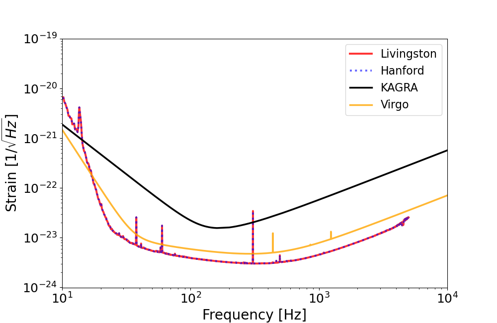
Figure 1: Comparison of representative sensitivity curves of the detectors employed in our simulations. The overlapping blue dotted and red full lines are the sensitivity curves of the Hanford and Livingston detectors with an optimal binary neutron star sensitivity range of 180 Mpc. The KAGRA curve, in black, and the Virgo one, in yellow, correspond to binary neutron star detection ranges of 25 and 115 Mpc, respectively. An equal mass neutron star binary with component masses of 1.4 M_⊙ was used to compute the horizon distance Chen et al. (2021).

To investigate the general trend of sky localization with respect to sensitivity range, we scale the sensitivity curves to the desired range. To do so, we multiply them by an arbitrary calibration factor until achieving that range with an error lower than 10^-2. We determine the horizon distance of the sensitivity curve using methods developed by Chen et al. (2021), simulating an equal-mass binary neutron star with component masses of 1.4 M_⊙. For KAGRA, we consider sensitivity range values between 5 and 25 Mpc, while for Virgo, we employ sensitivity curves ranging from 10 to 180 Mpc, approximately covering the expected sensitivity ranges of the two detectors for future observation runs Abbott et al. (2018b); Abe et al. (2022, 2023); Acernese et al. (2023). Although the scaling method employed for the spectral density curves provides only an approximation of the real curves, it allows for a first estimate of the performance of the detector networks, which could be refined in the future either with detector curves from real data for the specific horizon distance values or using a different scaling for each power law composing the PSD, e.g., a bigger scaling factor at lower frequencies for which the most improvements are expected soon.

Our primary focus is on assessing the impact of the KAGRA and Virgo detectors on the parameter estimation of gravitational wave signals assuming a fixed O4 LIGO network. To this end, we define the simulated source’s location relative to these two additional interferometers and vary only their sensitivity range while keeping that of the LIGO detectors constant at 180 Mpc. We use the antenna power pattern function $P(\theta,\phi)$ defined in Schutz (2011) as:

$$P(\theta,\phi) =F_{+}(\theta,\phi,\psi)^{2}+F_{\times}(\theta,\phi,\psi)^{2}$$ (1)

$$=\frac{1}{4}(1+\cos^{2}\theta)^{2}\cos^{2}2\phi+\cos^{2}\theta\sin^{2}2\psi,$$ (2)

where $F_{+}$ and $F_{\times}$ are called the sensitivity functions and $\theta$ and $\psi$ are the spherical coordinates with respect to the detector’s axes. We note that the antenna power pattern does not depend on the angle $\psi$ related to the polarization of the gravitational wave. It depends only on the relative orientation of the detector to the source, so that we obtain a wider sky coverage when interferometers are spread across the globe and have maximally different orientations. Table 1 presents the right ascension (RA), declination (DEC), and single detector antenna pattern function values for the source localizations maximizing and minimizing the antenna power pattern function for the KAGRA and Virgo detectors. We assume $\psi=0$ in the computation of the antenna power pattern function values. We show the location and orientation of the current network of ground-based detectors in Figure 2. We omit the GEO600 (Willke et al., 2002) detector as we do not include it in our analysis. The large distance between Virgo and KAGRA makes these extremely useful for sky-localization purposes in a four-detector network to obtain precise time-delay measurements.

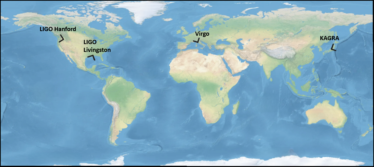
Figure 2: Location and orientation of the current network of gravitational-wave observatories, identified by the solid black lines. We omit GEO600 as we do not include it in our analysis.

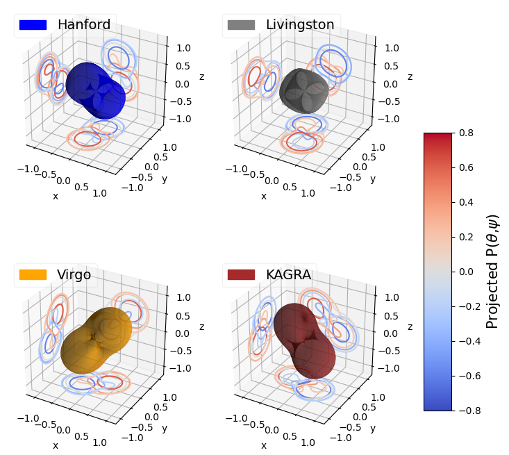
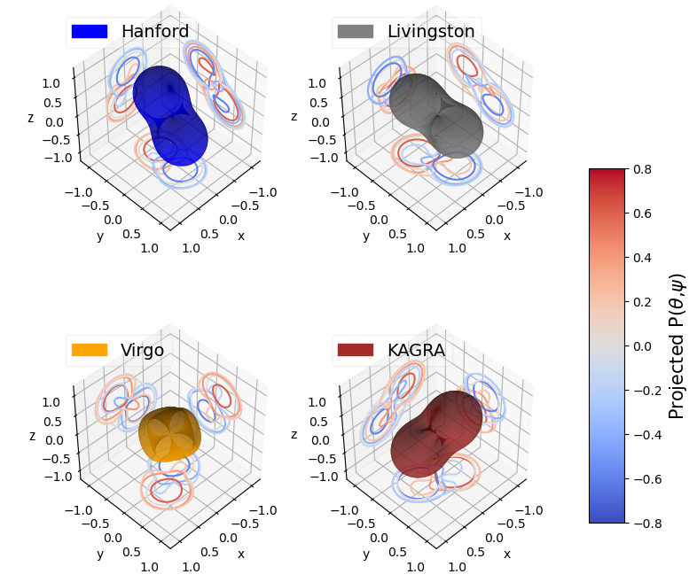
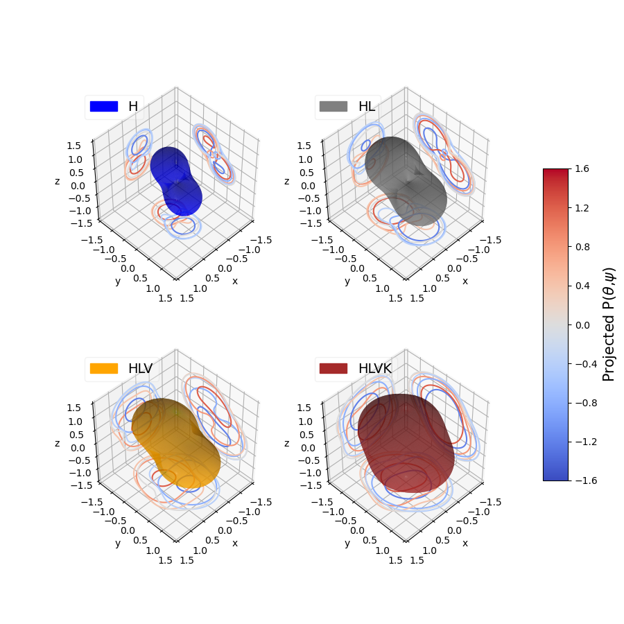
Figure 3: 3D visualizations of the antenna power pattern amplitude, from Eq. 2, for the LIGO-Hanford, LIGO-Livingston, Virgo and KAGRA detectors at a fixed arbitrary GPS time, so that the relative orientation of the detectors can be compared. The projections on the two-dimensional planes are the contours of the antenna power pattern amplitude for the projected axis.

Furthermore, in Figure 3 we show 3D visualizations of the antenna power pattern amplitude for the four employed detectors at a fixed GPS time from two different angles. We notice that all detectors have different relative orientations, agreeing with the different antenna pattern values presented in Table 1. While the two LIGO detectors are almost parallel, they are orthogonal to KAGRA and Virgo, which are also mutually orthogonal. In this work, we focus on the case in which KAGRA and Virgo have lower sensitivities than the two LIGO detectors. Their resulting lower signal-to-noise ratio could be partially compensated for some regions of the sky by their different relative orientations. From Table 1, we can compute an estimate of the fraction of LIGO’s sensitivity at which Virgo and KAGRA data would begin to have an effect on the sky localization constraints. This corresponds to the quotient between the single LIGO and the Virgo/KAGRA antenna power pattern amplitudes computed at the right ascension and declination values that maximize Virgo/KAGRA’s antenna power pattern. For Virgo, we find that the quotient is $\simeq 1/6$ so if the LIGO detectors have a sensitivity of 180 Mpc, we would expect to see significant improvements in the sky localization when Virgo reaches sensitivities $\simeq 30$ Mpc. For KAGRA, we find a similar quotient so that we expect improvements from 30-35 Mpc onwards, values which we do not include in this study. For all the values included in Table 1 we used the Bilby library Ashton et al. (2019) to compute the right ascension and declination for the maximum and minimum, respectively, P_max and P_min, of the antenna power pattern function at a specific arbitrary GPS time for each detector. In Appendix B we report the same values for P_best, the sky position maximizing the combined detector network antenna power pattern function for each configuration.

	RA (rad)	DEC (rad)	PK	PV	PH	PL
KAGRA Pmax	1.709	0.761	1.0	0.14	0.22	0.17
KAGRA Pmin	4.422	0.888	10-10	0.46	0.71	0.80
Virgo Pmax	5.785	0.761	0.24	1.0	0.17	0.14
Virgo Pmin	1.392	0.318	0.83	10-10	0.17	0.39

Table 1: Table of the right ascension (RA), declination (DEC) and the values of the single detector’s antenna pattern amplitude for the source localization maximizing and minimizing the antenna power pattern function, P_max and P_min respectively, for the KAGRA and Virgo detectors. The GPS time is fixed at 1379969683.0.

Given the source location values, to conduct each analysis we simulate a gravitational waveform and add it to a simulated interferometer data strain to capture the detector’s response (see Table 2 in Appendix A for the simulated parameter values). The process is facilitated using Bilby  Ashton et al. (2019); Romero-Shaw et al. (2020). The colored Gaussian noise background data is simulated from the PSD based on the scaled sensitivity curves, while the added waveform is generated using the LALSimulation library LIGO Scientific Collaboration (2018): we employ the IMRPhenomX family of phenomenological waveform models Pratten et al. (2020b). We use the simulated detector response and waveform to calculate the gravitational wave transient likelihood Whittle (1951). We then provide this likelihood to the Bilby sampler along with priors on relevant parameters, shown in Table 3 in the Appendix A, enabling a comprehensive parameter estimation. We opt for the dynesty sampler Speagle (2020), a nested sampling algorithm Skilling (2004) that employs differential evolution and adaptive sampling for an effective exploration of the high-dimensional parameter space. We summarize the configuration details for the dynesty sampler in Table 4 in Appendix A.

II.1 Post-processing

For the gravitational wave signals from highly-spinning binary black hole mergers, we want to understand if a larger and more sensitive detector network would allow us to better constrain the source’s intrinsic parameters (see Sec. V), while in the non-spinning binary black hole and binary neutron star cases, we want to quantify the improvements in determining the sky localization. We focus on the sky localization area as we expect it to be influenced the most by adding a new detector to the network (Fairhurst, 2011). Indeed, the additional detector does not have a comparable or higher sensitivity range that would enhance the source parameter estimation results. Nevertheless, its distant location to the LIGO detectors allows for a significant gain in time-delay information which can be used for triangulation purposes. To this end, from the parameter estimation results of the non-spinning system’s mergers, we generate a sky map, a graphical representation of the probable source locations of a gravitational wave event on the celestial sphere. We do this by passing the posterior probability samples of the distance, right ascension, and declination to the ligo.skymap function lig (2022). Subsequently, we extract the values corresponding to the 90% probability contours of the sky localization area from the generated sky map. To address the stochastic nature of the sampling process and Gaussian noise, and consequently, the variability in sky localization area results, we conduct multiple simulations with identical configurations and different realizations of Gaussian noise and then report a statistical summary. By subjecting the obtained results to a two-component Gaussian mixture model algorithm, we derive the probability distribution function (pdf) characterizing the spatial distribution of sky area in relation to sensitivity range Pedregosa et al. (2011). We chose the two-component model as it proved to be the best to mirror the distribution of the underlying data, independently of the latter’s features. Employing this estimated pdf, we generate 20,000 samples of sky area and range sensitivity values. Subsequently, we apply a filtering criterion, retaining samples falling within the 5th and 95th percentiles and featuring positive (physical) values for both coordinates. Lastly, we classify data points into bins based on the sensitivity range values, aligning the bin edges with integer values. When varying KAGRA’s sensitivity range, we will employ unitary bin-widths, while when varying Virgo’s sensitivity range, we use quinary band-widths.

III Results of Zero Spin Binary Black Hole Simulations

We simulate gravitational wave signals from non-spinning binary black hole mergers using the IMRPhenomXPHM waveform approximant for both the signal’s simulation and the likelihood evaluation Pratten et al. (2021). We simulate equal-mass black holes with a detector-frame chirp mass $\mathcal{M}$ of 50 M_⊙, where

$$\mathcal{M}=\frac{(m_{1}m_{2})^{3/5}}{(m_{1}+m_{2})^{1/5}},$$ (3)

with m_1/2 denoting the detector-frame mass of the two compact objects. The source is placed at a distance of 2000 Mpc from us. The complete list of parameter values can be found in the first column of Table 2 in Appendix A. Following the procedure outlined in Sec. II, we perform six simulations and full parameter estimation runs for each sensitivity range value, and post-process the results into sky localization area values using a Gaussian Mixture model. The results are presented in Figure 4.

In Figure LABEL:fig:HLK_bbh, we show the evolution of the mean and 90 % probability contours of the sky area, dots and squares, and shaded area, respectively, for the HL-K detector network varying the range sensitivity of the KAGRA detector only. Henceforth, we will separate with a dash the letter referring to the detector of the network whose range sensitivity we have varied for the specific plot. The brown and orange points and areas were obtained by placing the source in the P_max and P_min source location, respectively, for the KAGRA detector (see Table 1). The black dotted line corresponds to the field of view of the Zwicky Transient Facility. By 0 Mpc we refer to the results obtained with the two LIGO detectors only at a fixed sensitivity range of 180 Mpc. For all the following sky area plots, we computed the 0 Mpc value with the same detector network used for the other sensitivity values but excluding the detector whose sensitivity range is varied. For Figure LABEL:fig:HLK_bbh, while in the P_max location case, the mean sky area value decreases notably, when increasing KAGRA’s sensitivity range, it remains roughly constant in the P_min location case. The decrease of the mean sky area is most significant from $\sim$10 Mpc on-wards.

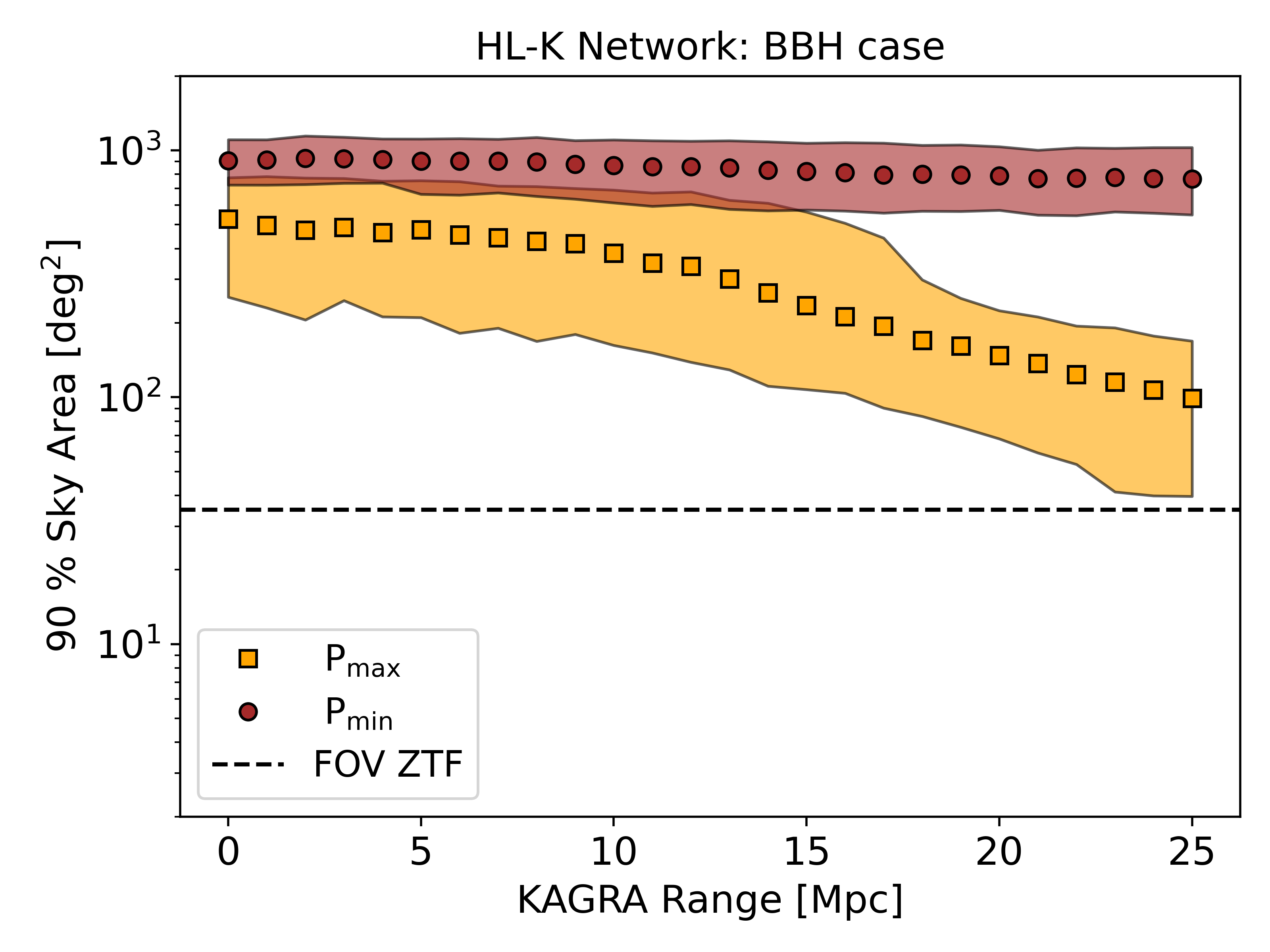
(a)

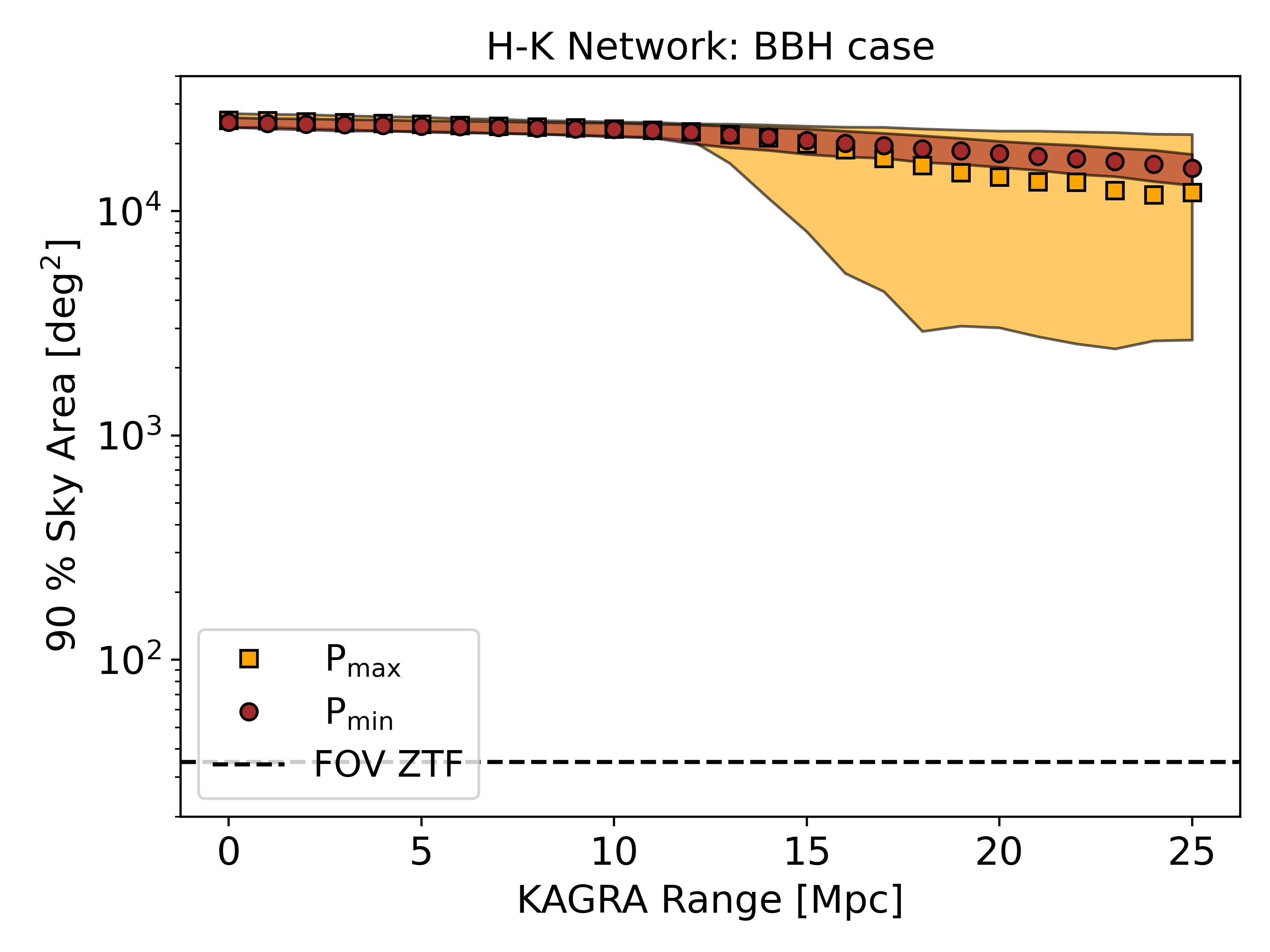
(b)

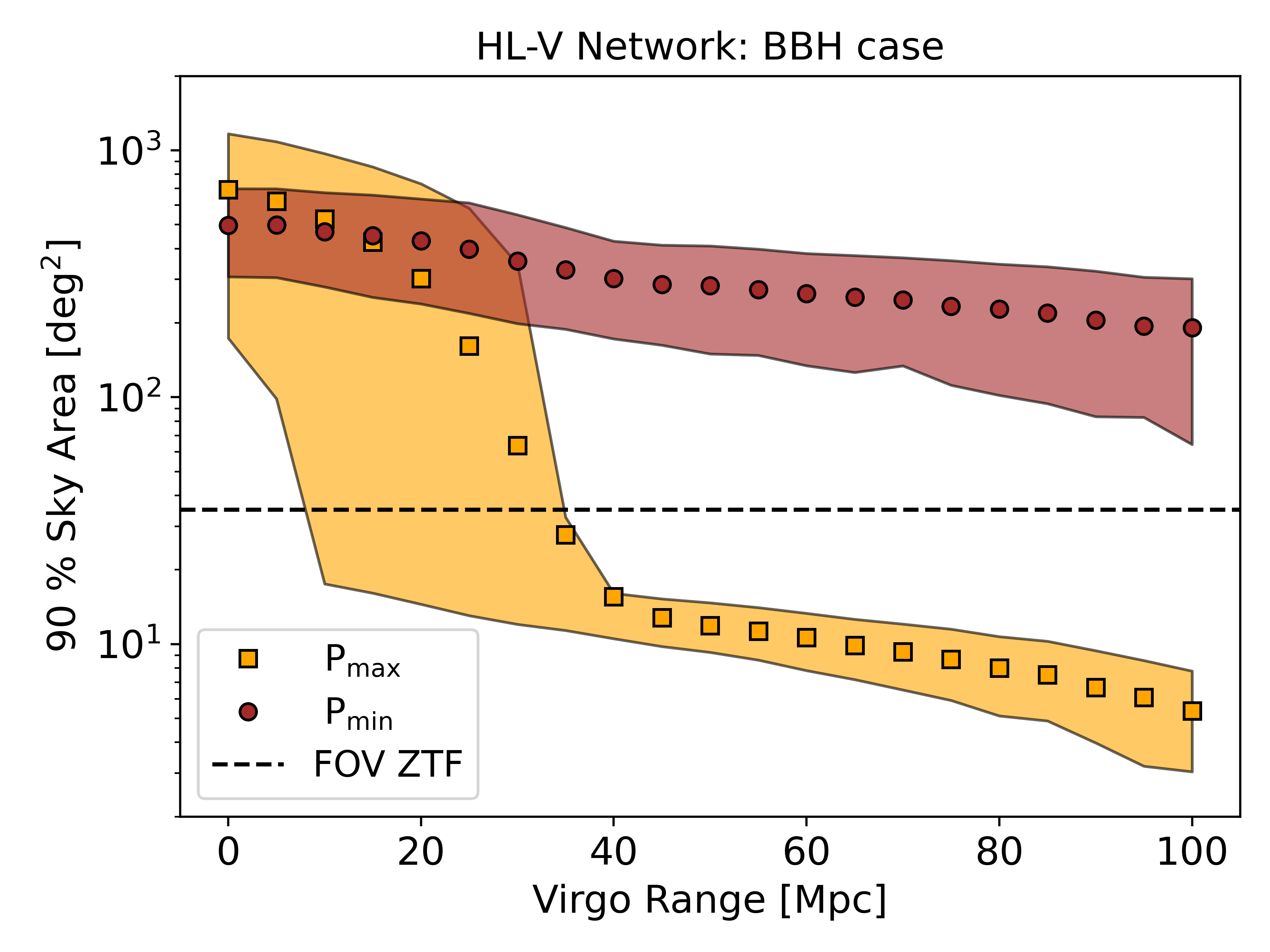
(c)

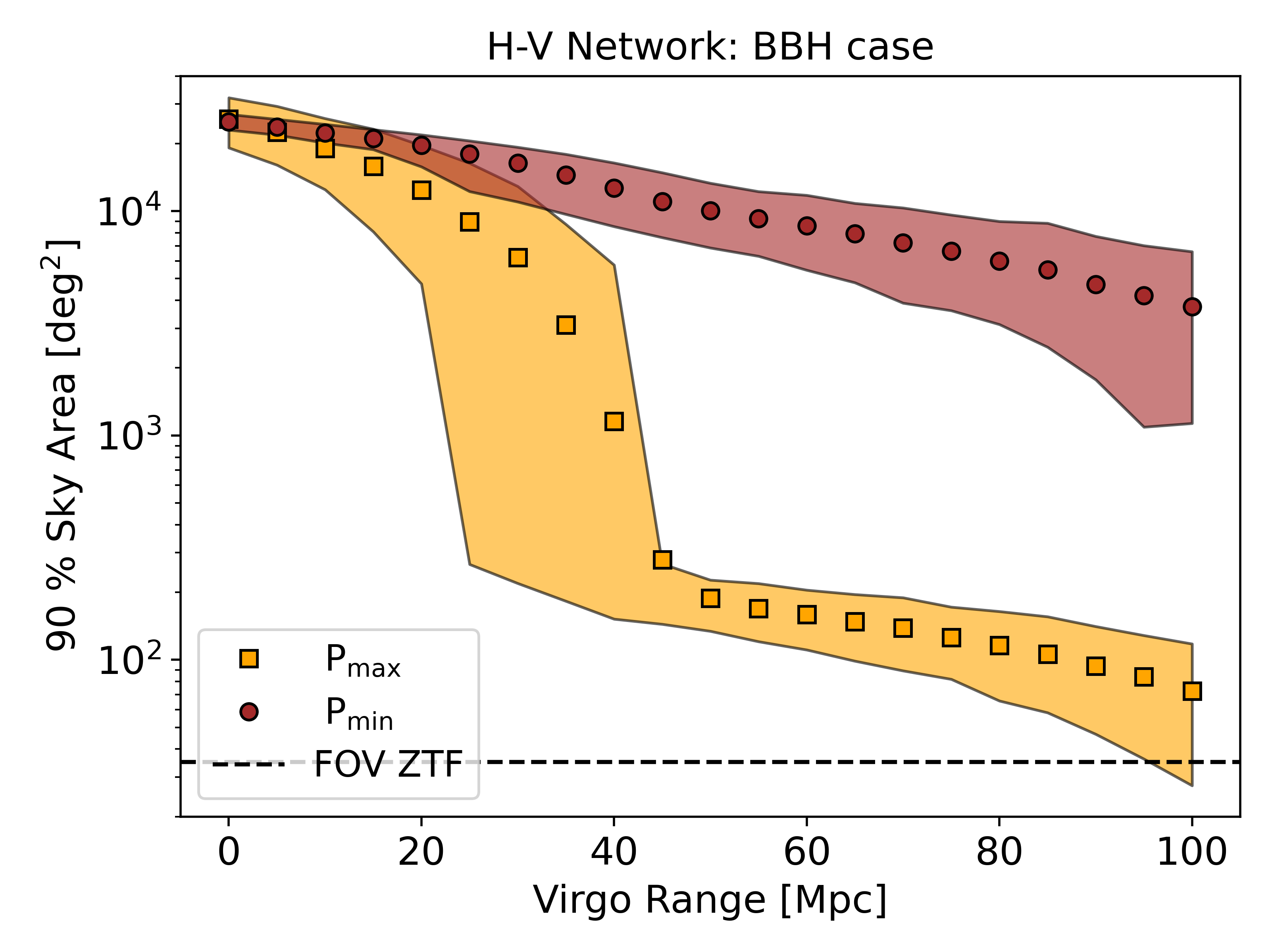
(d)

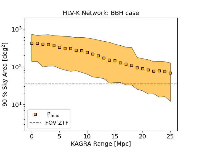
(e)

Figure 4: Zero-Spin Binary Black Hole Simulations
The mean and the 90 % probability contour of the sky area for varying detector range sensitivity values for a gravitational wave signal emitted by a binary black hole coalescence from the P_max and P_min source location for the least sensitive detector, brown and orange points and areas respectively. The points, brown dots, and orange squares, represent the mean value, and the areas stretch from the 5% to the 95% quantiles for each sensitivity range bin. The black dotted line corresponds to the field of view of the Zwicky Transient Facility. We obtained the 0 Mpc points from simulations excluding the least sensitive detector. We fixed the range sensitivity of the two LIGO detectors at 180 Mpc. (a): Varying the KAGRA detector and employing the LHK network. (b): Varying the KAGRA detector and employing the HK network. (c): Varying the Virgo detector and employing the LHV network. (d): Varying the Virgo detector and employing the HV network. (e): Varying the KAGRA detector and employing the LHVK network. Virgo’s sensitivity is fixed at 30 Mpc.

Figure LABEL:fig:LK_bbh shows the sky area results for the P_max and P_min source locations for the H–K detector network varying the KAGRA sensitivity range. For the P_max case, the sky area improves considerably after $\sim$15 Mpc, with the 90% quantiles spanning to one order of magnitude lower values than in the P_min case. Also the latter improves slightly from 15 Mpc on-wards. The mean sky area values for the P_max case are of the order $1.5\times 10^{4}$ deg², when KAGRA has a 25 Mpc sensitivity range, compared to $2\times 10^{4}$ deg² for the P_min case. The overall improvement is not significant for precisely localizing the source, and the sky area values are two orders of magnitude higher than for the corresponding three-detector network HL–K.

In Figure LABEL:fig:HLV_bbh, we report the same quantities as in Figure LABEL:fig:HLK_bbh, but for the HL–V detector network, using the P_max and P_min source location for the Virgo detector. We can see a clear difference between the P_max and P_min distributions, with the decrease in sky area being almost two orders of magnitude more in the former source location case. We notice how the Virgo detector with a sensitivity range of 35 Mpc and above would provide a significant improvement, reducing the mean sky area to $\sim$10 Mpc. With a Virgo detector range sensitivity between 25 and 35 Mpc, the inferred sky area improves considerably, although it exhibits a high variability. In the P_min case, the improvement in sky area is less remarkable as the mean changes from $\sim$600 deg² with the HL detector network to $\sim$250 deg² for the LH–V network when Virgo has a sensitivity range of 100 Mpc.

The corresponding two-detector network, H–V, results are shown in Figure LABEL:fig:LV_bbh. We notice that both the P_max and P_min distributions follow a similar trend to the ones obtained for the HL–V detector network. In the P_max case, we see the most significant improvement in sky area for sensitivity range values between 25 and 45 Mpc. In this range, the mean sky area value drops from $\sim$10⁴ to $\sim$200 deg². From 45 Mpc onwards, the betterment of the mean sky area value is not as meaningful, reaching $\sim$80 deg² when Virgo has a sensitivity range of 100 Mpc. In the P_min case, the distribution of the mean sky area values is quasi-linear, progressing continuously from $\sim$2$\times$10⁴ to 400 deg² for 0 and 100 Mpc respectively.

Finally, Figure LABEL:fig:HLVK_bbh shows the mean sky area values and 90% probability contours obtained with the methods outlined in Sec. II.1 from simulated detections of binary black hole merger signals with the HLV-K detector network when varying the sensitivity range of the KAGRA detector only. We fix the sensitivity of the Virgo detector at 30 Mpc and employ the P_max source location for the KAGRA detector in all the runs. We observe a continuous improvement of the sky area from 5 to 25 Mpc, with the mean value passing from $\sim$500 deg² to $\sim$100 deg². This suggests that even in a four-detector network, adding an interferometer up to ten times less sensitive than the others but at a different spatial location and with a different relative orientation leads to a 75% reduction in the mean sky localization area inferred with the network.

IV Results of Binary Neutron Star Simulations

We simulate gravitational wave signals from non-spinning binary black hole merger following the same procedure of Sec. III. The binary neutron stars are placed at a distance from Earth of 100 Mpc and have a chirp mass of $1.198$ M_⊙, comparable to the first binary neutron star merger event GW170817 Abbott et al. (2017e). The complete list of parameter values can be found in the second column of Table 2 in Appendix A. For the gravitational wave signal simulation and parameter estimation, we use the IMRPhenomPv2 Hannam et al. (2014) waveform approximant, and to speed up the evaluation of the likelihood function, we employ the reduced order quadrature basis from the analysis of GW170817 Canizares et al. (2013). We list the priors in the second column of Table 3. The results are presented in Figure 5.

In Figure LABEL:fig:HLK_ns, we show the mean and the 90% quantile region of the sky localization area as a function of the sensitivity range of the KAGRA detector for the P_max and P_min source locations for KAGRA. We use the same color scheme as in Sec. III. The points and regions have been obtained with the methods detailed in Sec. II.1 from the parameter estimation results of simulated gravitational wave signals emitted by the coalescence of binary neutron star mergers using the HL–K detector network. The 0 Mpc point corresponds to the sky area obtained from an HL detector network run with identical source locations and parameters. While in the P_min source location case, there is no improvement in the mean sky area value from 0 to 25 Mpc, in the P_max case, the value decreases continuously from $\sim$200 deg² to $\sim$30 deg² for the same range values.

Figure LABEL:fig:LK_ns shows the sky area results for the P_max and P_min source locations for the H–K detector network, varying sensitivity range of KAGRA. For the P_max case, the sky area improves from $\sim$15 Mpc onwards, with the 90% quantiles spanning to one order of magnitude lower values than in the P_min case. The mean sky area values for the P_max case are of the order $1.2\times 10^{4}$ deg², with KAGRA having 25 Mpc range sensitivity, compared to $1.5\times 10^{4}$ deg² for the P_min case. This trend is coherent with the corresponding binary black hole case shown in Figure LABEL:fig:LK_bbh.

Figure LABEL:fig:HLV_ns shows the mean sky area values and the 90% probability areas obtained from the parameter estimation runs using the HL–V detector network placing the source in the P_max and P_min source locations for Virgo. As in Figure LABEL:fig:HLV_bbh, we see that for the P_min source location, the sky area values do not improve when Virgo’s sensitivity range is wider, while in the P_max case, there is an improvement starting from 15 Mpc. This improvement is significant up to $\sim$40 Mpc, going from $\sim$200 deg² without Virgo to $\sim$4 deg² when Virgo has a range sensitivity of 40 Mpc. The sky area values remain roughly constant from 40 Mpc to 100 Mpc for this optimal case. In the P_min case, the sky area does not change between 0 and 40 Mpc and decreases minimally from 40 Mpc on-wards.

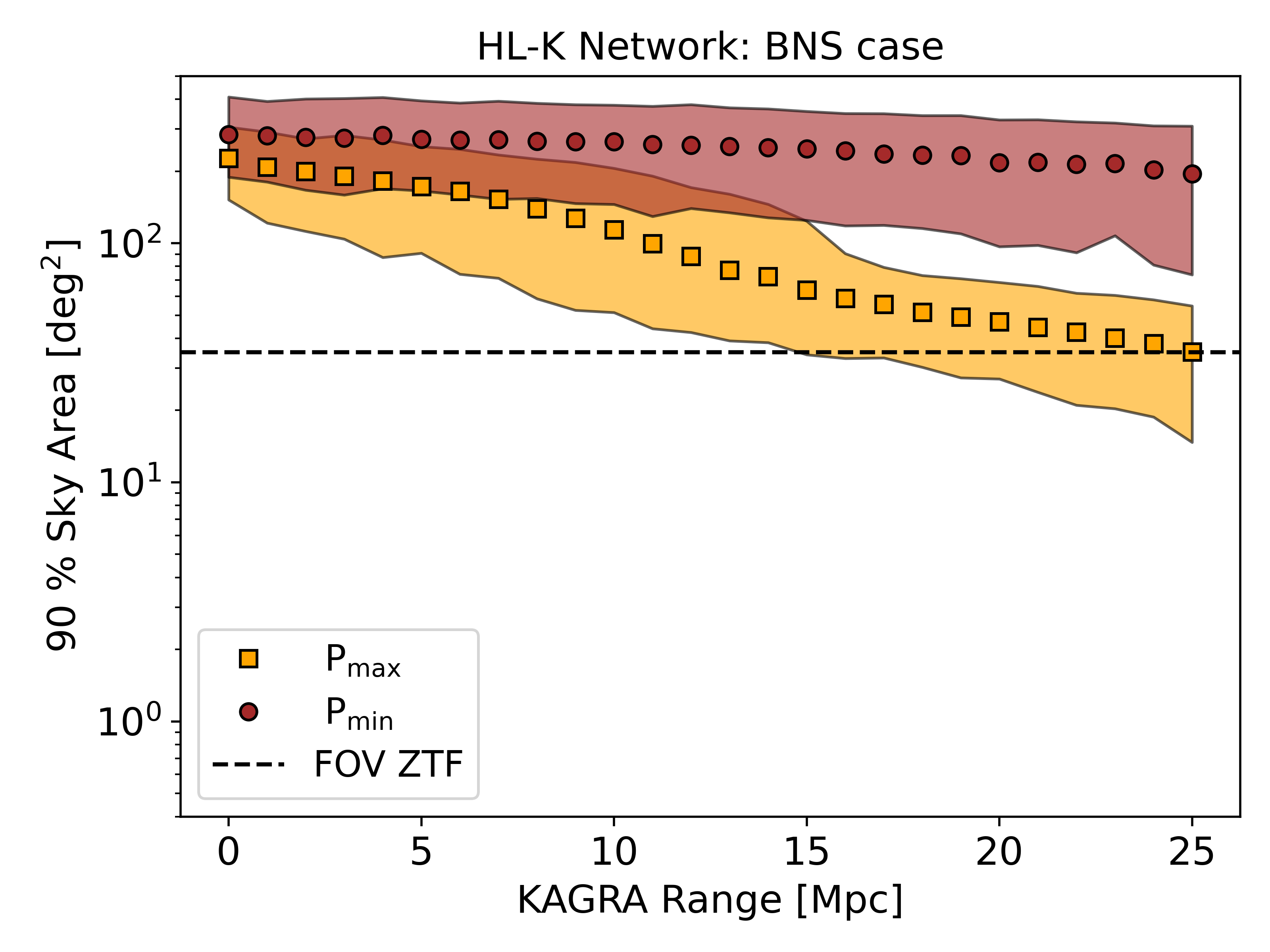
(a)

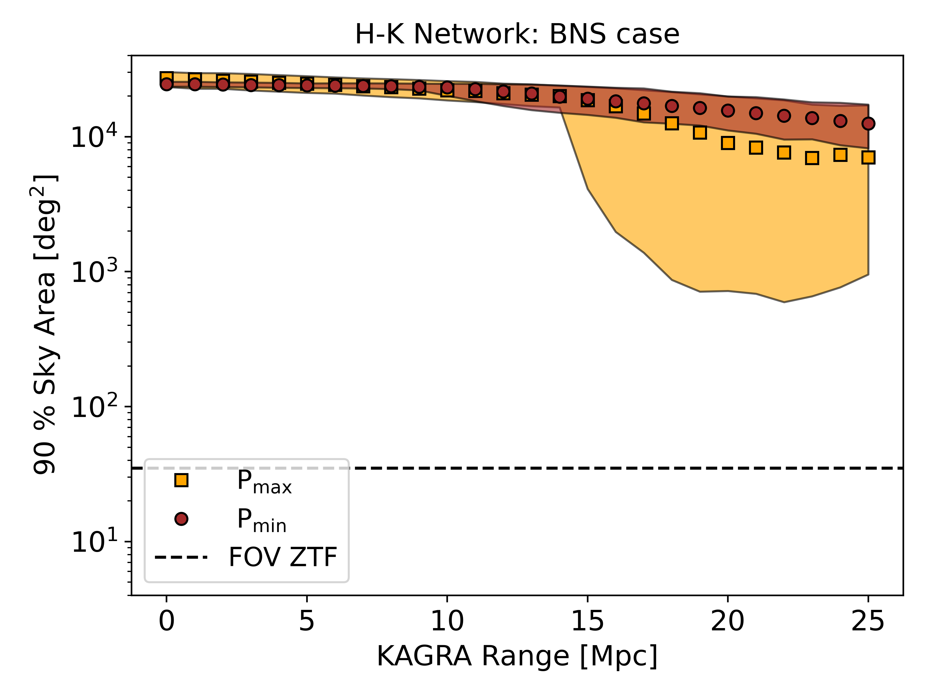
(b)

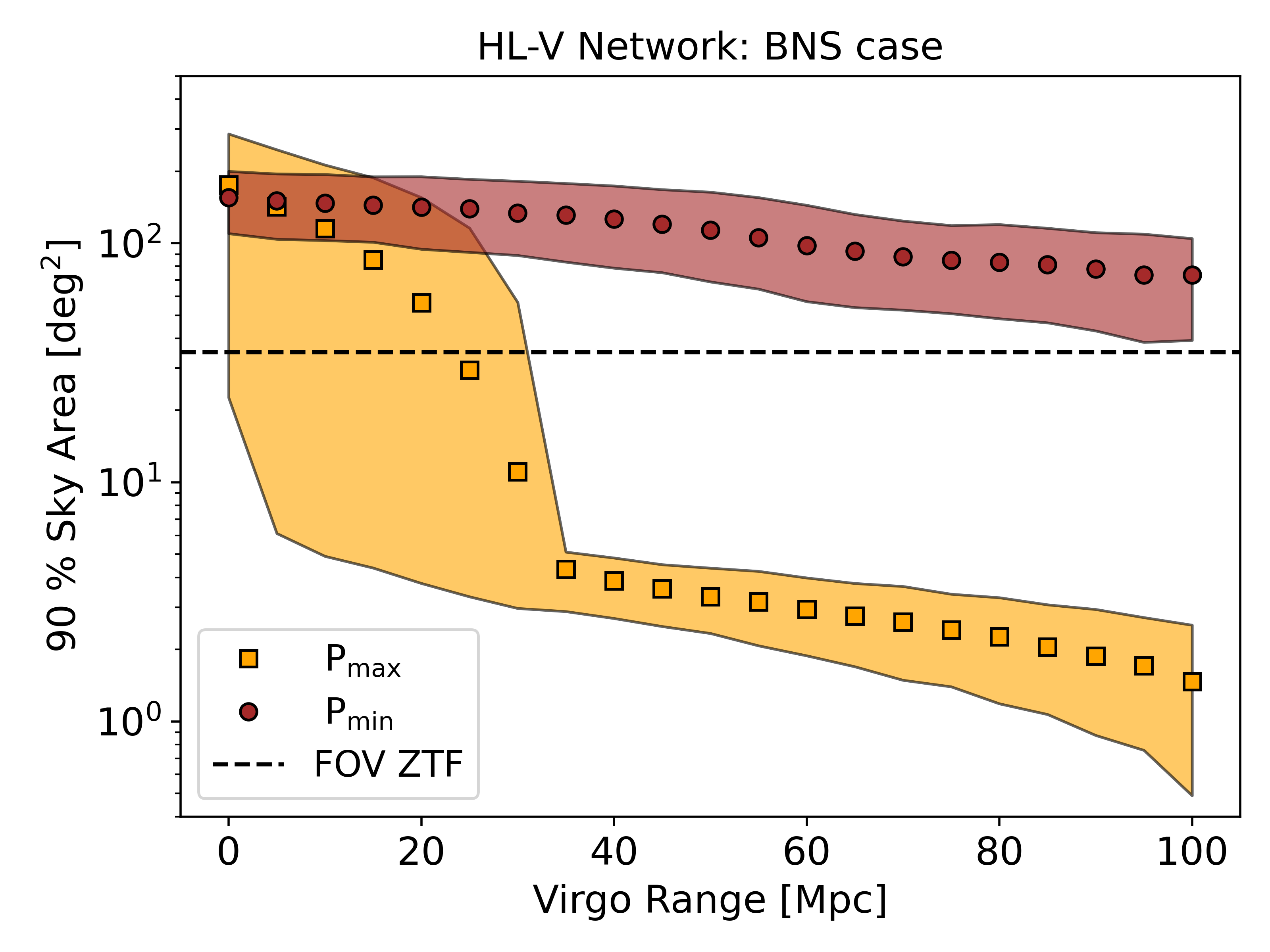
(c)

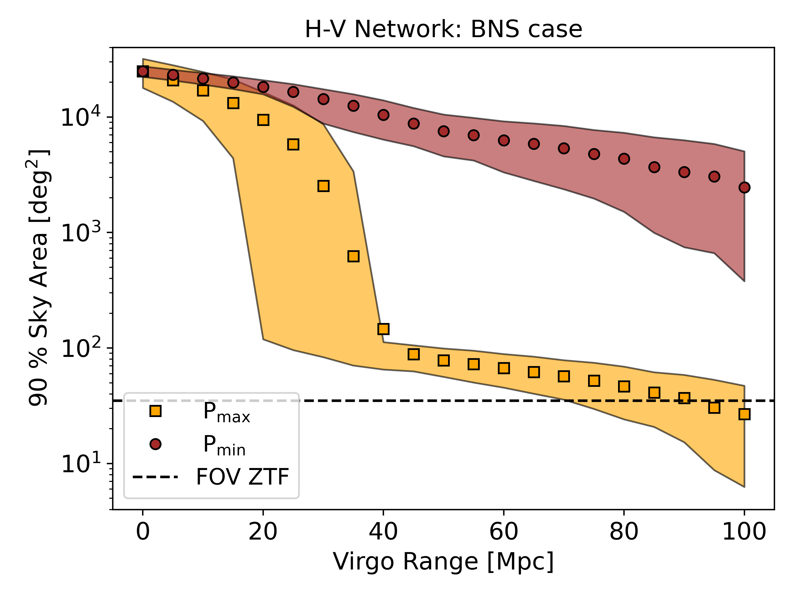
(d)

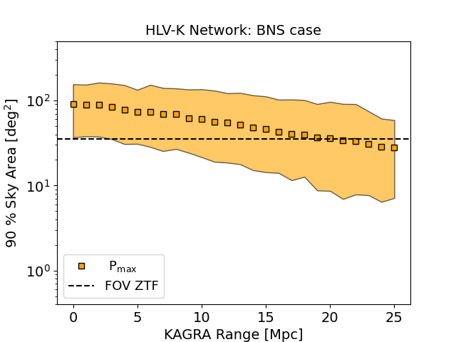
(e)

Figure 5: Binary Neutron Star Simulations
The mean and the 90% probability contour of the sky area for varying detector range sensitivity values for a gravitational wave signal emitted by a binary neutron star coalescence from the P_max and P_min source location for the least sensitive detector, brown and orange dots, and areas, respectively. The dots represent the mean value, and the areas stretch from the 5% to the 95% quantiles for each sensitivity range bin. The black dotted line corresponds to the field of view of the Zwicky Transient Facility. We obtained the 0 Mpc points from simulations excluding the least sensitive detector. We fixed the range sensitivity of the two LIGO detectors at 180 Mpc. (a): Varying the KAGRA detector and employing the LHK network. (b): Varying the KAGRA detector and employing the HK network. (c): Varying the Virgo detector and employing the LHV network. (d): Varying the Virgo detector and employing the HV network. (e): Varying the KAGRA detector and employing the LHVK network. Virgo’s sensitivity is fixed at 30 Mpc.

As for the BBH case, the sky area for the two detector networks, H–V, exhibits a similar evolution for the sensitivity range of Virgo. These results are visible in Figure LABEL:fig:LV_ns. In the optimal case, we see a considerable refinement of the sky area between 25 and 40 Mpc, with the mean value passing from 10⁴ to 10² deg². This value continues to improve continuously up to 30 deg² at 100 Mpc. Also in the P_min case, differently from the correspondent three detector network results in Figure LABEL:fig:HLV_ns, we see a noticeable improvement with increasing sensitivity range. Indeed, the mean sky area value is reduced to 3$\times$10³ deg² at 100 Mpc, with the 90% area reaching down to 400 deg², from 2.5$\times$10⁴ at 0 Mpc.

Lastly, Figure LABEL:fig:HLVK_ns is the correspondent of Figure LABEL:fig:HLVK_bbh for simulated detections of binary neutron star merger signals with the HLV–K detector network when varying the sensitivity range of the KAGRA detector only. The network setup in the simulations is identical to the binary black hole case. Similarly, we observe a continuous improvement of the sky area, with the mean value decreasing from $\sim$100 deg² to $\sim$30 deg². The 90% quantile region follows a similar trend, with the lower end going from $\sim$40 deg² without KAGRA to $\sim$5 deg² when KAGRA reaches a sensitivity range of 25 Mpc.

V Results of highly-spinning binary black holes

Finally, we simulate gravitational wave signals from highly spinning aligned binary black holes employing the Hanford-Livingston-Virgo detector network and perform parameter estimation varying the range sensitivity of the Virgo detector only. In contrast to the previous sub-section, we aim to understand how the sensitivity of the Virgo detector impacts the inference of the intrinsic properties of the source. We focus on a high-spin binary black hole merger as the spin-related parameters, e.g., the effective spin and the individual spin magnitudes, are only broadly constrained by current detector network configurations, while they encode a large amount of information. Tighter constraints on these variables could lead to an enhanced understanding of the Universe’s black hole population properties and their formation channels (Bavera et al., 2020).

We simulate a signal with the following arbitrary choice of parameters: we employ a chirp mass of 27.93 M_⊙ and a $\chi_{\rm eff}$ value of 0.91, and assume that the spins are aligned so that $\chi_{p}=0$ and the tilt angles are null. The complete list of values is reported in the third column of Table 2 in Appendix A, while the priors used for the runs are listed in the third column of Table 3. We also adjust the settings for the dynesty sampler, as visible in Table 4 in Appendix A, to reduce the bias in the posterior probability results.

The analysis of these simulations takes significant computational effort. To alleviate this, we will apply a rejection sampling approach using a base analysis as a proposal distribution and reweighting for each rescaled Virgo sensitivity. Specifically, we begin with the posterior obtained for the HLV network when Virgo has a sensitivity of 50 Mpc and apply the standard Nested Sampling algorithm as described in Section II. We choose 50 Mpc, as this is above the point where the extrinsic parameters are well constrained by triangulation. This initial HLV analysis takes $\approx 8$ hrs using 30 CPU cores. Each reweighting takes $\approx 10$ minutes on a single CPU core. This vast improvement is only possible because as we increase the sensitivity of Virgo, the posterior narrows marginally such that the base analysis is an excellent generating distribution.

After performing the base analysis and obtaining a set of posterior samples $\{\theta_{i}\}$, we obtain the weight for the $i$th sample as

$$W_{i}=\frac{f(\theta_{i})}{Mg(\theta_{i})},\quad\text{with}\quad f(\theta_{i})\leq M\times g(\theta_{i}),$$ (4)

where $g(\theta_{i})$ is the generating distribution, $f(\theta_{i})$ is the resampling distribution, and $M$ is a factor used to ensure that the generating distribution encompasses the resampling distribution, effectively normalizing the weights to the range $[0,1)$. In our case, the generating distribution is $g(\theta_{i})=\mathcal{L}(\theta_{i}|\rm{H_{180}})\mathcal{L}(\theta_{i}|\rm{L_{180}})\mathcal{L}(\theta_{i}|\rm{V_{50}})\pi(\theta_{i})$, while the resampling distribution is $f(\theta_{i})=\mathcal{L}(\theta_{i}|\rm{H_{180}})\mathcal{L}(\theta_{i}|\rm{L_{180}})\mathcal{L}(\theta_{i}|\rm{V_{j}})\pi(\theta_{i})$ where the subscripts for the detectors indicate the sensitivity range, expressed in Mpc, of the PSDs used for the evaluation of the noise realizations and $j$ ranges from 60 to 180 Mpc. Therefore, since the likelihood for the Hanford and Livingston data is identical, we can simplify the weights from Eq. 4 to be:

$$W_{i}=\frac{\mathcal{L}(\theta_{i}|\rm{V_{j}})}{M\mathcal{L}(\theta_{i}|\rm{V_{50}})}.$$ (5)

The basic idea of rejection sampling is to draw random samples from the generating distribution $g$, calculate the related weights, and compare these to a random number taken from a uniform distribution between 0 and 1 (Casella George and T., 2004). If the weight is bigger than the random number, we accept the sample and include it in the posterior, otherwise, we discard it. It is important to carefully choose the value of $M$ so that it satisfies the condition in Eq. 4 and at the same time does not make the sampling inefficient by being too large. We choose the value of $M$ by calculating

$$\log(M)=\mathrm{Max}_{i}\left(\frac{\log(\mathcal{L}(\theta_{i}|\mathrm{V_{j}}))}{\log(\mathcal{L}(\theta_{i}|\mathrm{V_{50}}))}\right)+0.1\,,$$ (6)

over set of samples.

To account for the high variability of the individual noise realizations when using the same PSD and the resulting oscillating efficiencies, for each sensitivity range value we perform 20 iterations of the resampling routine. We focus on the sensitivity range between 50 and 180 Mpc and employ PSDs obtained with the methods described in Section II progressively increasing the sensitivity by tens. We then combine the samples from the multiple iterations before post-processing the data.

In Figure 6 we show a summary of our results. In each of the panels, we show the mean, blue dots, and 90% probability contours, red lines, of the selected parameter versus the different sensitivity ranges of the Virgo detector. The 90% contour is centered around the mean for all variables except for $\chi_{\rm{p}}$. To account for the latter’s true value corresponding to the boundary of the parameter’s lower constraint, its 90% contour is taken from the lower boundary to the 90% quantile. The true values used for the simulation of the gravitational wave signal correspond to the black dotted horizontal lines. Overall, we notice a consistent improvement in the mean value and a tightening of the 90% probability contours when increasing Virgo’s sensitivity. This trend is particularly evident in panels LABEL:fig:chirp_mass and LABEL:fig:chi_eff, depicting the results for the detector-frame chirp mass and the effective spin parameter. The latter is a dimensionless parameter quantifying the alignment of the spins of the binary components are given by:

$$\chi_{\rm{eff}}=\frac{(m_{1}\cdot\chi_{1}+m_{2}\cdot\chi_{2})\cdot\hat{L}}{M},$$ (7)

with $m_{1/2}$ denoting the masses of the two black holes, M their total mass, L their angular momentum and $\chi_{1/2}$ the individual dimensionless spins. For both, the chirp mass and effective spin, the mean value gets continuously closer to the true value reaching a 60% and 45% improvement at 180 Mpc, respectively. At the same time, the 90% probability contours decrease by 30% for both parameters from 60 to 180 Mpc. The mass ratio shown in panel LABEL:fig:mass_ratio shows a similar trend going from 60 to 180 Mpc, with a 60% improvement in the mean value and a 30% decrease in the 90% probability contour. We notice that in this case, the most significant betterments happen at sensitivities above 100 Mpc. Finally, in panels LABEL:fig:chi_p and LABEL:fig:ra we report the results for $\chi_{p}$ and the right ascension, respectively. The parameter $\chi_{p}$, introduced in Schmidt et al. (2012), combines the spin magnitudes and their relative orientation to the total angular momentum, effectively characterizing the degree of precession in a binary black hole system. As we are analyzing a non-precessing binary system, we expectedly recover $\chi_{p}$ to be consistent with zero at all sensitivities. For the right ascension, we obtain only minor improvements passing from 60 to 180 Mpc. This is not surprising because, as noted in Section III, the sky-localization shows the largest improvements at sensitivities between 20 and 40 Mpc. Overall, we can conclude that when Virgo reaches sensitivities starting from approximately half of the LIGO sensitivities, i.e. 90/100 Mpc, the inference of the intrinsic source parameters improves significantly.

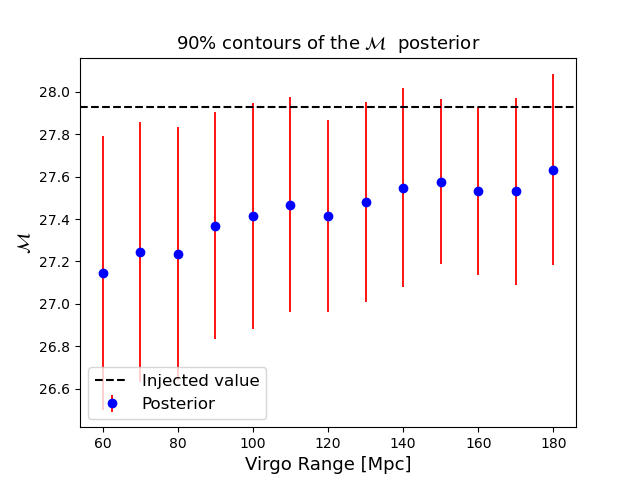
(a)

(b)

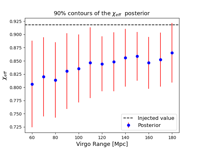
(c)

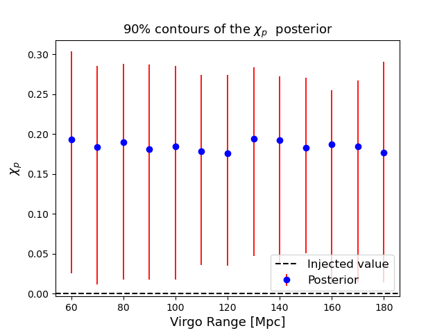
(d)

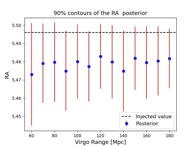
(e)

Figure 6: High-Spin Binary Black Hole Simulations
The mean, blue dots, and 90% posterior probability contour, red line, of the detector-frame chirp mass obtained varying the sensitivity range of Virgo in the parameter estimation analysis of a simulated high-spin binary black hole merger signal. We employ the HL-V detector network, fixing the sensitivity range, noise realization and detector response of the two LIGO detectors. The black dotted line represents the true chirp mass value of the simulated signal.

VI Minimum frequency study

Gravitational wave signals from merging black holes and neutron stars sweep up in frequency during the inspiral stage before their eventual merger and ringdown. From a simple post-Newtonian calculation, it can be shown (see, e.g. Peters and Mathews (1963)) that the time-to-merger from a frequency $f_{0}$ is

$$t_{m}=1.5\,\textrm{s}\left(\frac{20\,M_{\odot}}{\mathcal{M}}\right)^{5/3}\left(\frac{20\,\textrm{Hz}}{f_{0}}\right)^{8/3}\,,$$ (8)

where $\mathcal{M}$ is the detector-frame chirp mass defined in Eq. 3. The power of $8/3$ means that signals spend far longer at lower frequencies than at the higher frequencies near the merger (this expression breaks down near the merger itself but is a good approximation for the early inspiral). However, the noise curve of the detector steeply rises at low frequencies due to seismic noise. As such, analyses often assume a minimum frequency $f_{\rm min}$ below which the signal has negligible contributions.

Specifically, in standard approaches to Bayesian inference for signals, we assume a stationary Gaussian noise resulting in a log-likelihood:

$$\log\mathcal{L}(d|\theta)\propto\sum_{k}\frac{2|\tilde{d}_{k}-\tilde{\mu}_{k}(\theta)|^{2}}{TS_{k}}\,,$$ (9)

where $T$ is the data duration, $k$ is the index of the frequency bin, $\tilde{d}$ is the complex frequency-domain data, $\tilde{\mu}(\theta)$ is the frequency-domain source model evaluated at a set of source parameters $\theta$, and $S$ is the Power Spectral Density (see, e.g., Finn (1992); Veitch et al. (2015)). In practice, the minimum frequency is implemented by neglecting to sum components below $k_{\rm min}$, the frequency bin associated with $f_{\rm min}$.

The introduction of $f_{\rm min}$ then informs the choice of $T$, the duration of data to analyze. Choosing $T$ to be much larger than the actual signal duration is inefficient, requiring unnecessary computation and ultimately increasing the computational cost of an analysis. The standard in the field remains to take $f_{\rm min}=20$ Hz and then choose $T$ to be the next power of two greater than the estimated time-to-merger (either using Eqn. 8 or an improved model incorporating other physical effects).

This standard has been in place since the first detection (Abbott et al., 2016c), though with some exceptions. It is common to increase $f_{\rm min}$ as a mechanism to mitigate non-Gaussianity in the detector (Davis et al., 2022). However, it has also been decreased to maximize the number of cycles in-band for analysis (see, e.g., Abbott et al. (2020f) and Abbott et al. (2020d) which used a minimum frequency of 19.4 Hz and 11 Hz, respectively).

While the $20$ Hz rule of thumb is built on a solid understanding of the detector performance over the first observing runs, recent upgrades have seen improvements in the low-frequency sensitivity and future detector developments aim to improve performance further. This leads us to ask: what conditions should be met for $f_{\rm min}$ to be decreased? Our ultimate goal is to develop a simple-to-compute metric that can provide gravitational-wave astronomers with a better-informed rule of thumb for choosing $f_{\rm min}$.

To construct our metric, we use the matched-filter Signal-to-Noise-Ratio (SNR)

$$\rho_{\rm mf}=\frac{\langle\tilde{d},\tilde{\mu}(\theta)\rangle}{\sqrt{\langle\tilde{\mu},\tilde{\mu}(\theta)\rangle}}\,,$$ (10)

where $\langle a,b\rangle$ denotes the noise-weighted inner product:

$$\langle a,b\rangle=\frac{4}{T}\sum_{k=k_{\rm min}}^{k_{\rm max}}\Re\left(\frac{a_{k}b_{k}^{*}}{S_{k}}\right)\,,$$ (11)

and $k_{\rm min}$ corresponds to the minimum frequency bin $f_{\rm min}$ while $k_{\rm max}$ corresponds the maximum frequency bin (which we set to $2048$ Hz).

Taking time-domain data from a given detector, we Fourier transform to the frequency domain and add to it a simulated fiducial signal; we then use that same signal to calculate the matched-filter SNR. I.e., the simulated signal added to the data is also used in Eqn. 10.

Finally, we vary $f_{\rm min}$ and define $\hat{f}_{\rm min}$ to be the minimum frequency at which $\rho_{\rm mf}$ decreases by $\epsilon=0.1\%$ relative to the value as calculated at $f_{\rm min}=15$ Hz (an arbitrary choice considered to be sufficiently low to represent the maximum SNR). Within this definition, there are two tuning parameters. First, the choice of fiducial signal. We apply two choices: a fiducial BBH and a fiducial BNS. For both signals, we use the IMRPhenomXAS waveform model (Pratten et al., 2020b) with zero-spin, equal masses, and arbitrary choices of $\theta_{\rm JN}=0.4$, $\psi=2.659$, $\phi=1.3$, $\alpha=1.375$, $\delta=-1.2108$ for the inclination angle, polarisation angle, phase, right-ascension, and declination. The two differ only in the choice of chirp mass and luminosity distance for which we use $30$ $M_{\odot}$ and $500$ Mpc for the BBH case and $2$ $M_{\odot}$ and $50$ Mpc for the BNS case. The second tuning parameter is $\epsilon$, which sets the threshold loss of SNR. Choosing $\epsilon$ to be arbitrarily small simply recovers the minimum allowed frequency, i.e. $15$ Hz. We choose $0.1\%$ as a conservative estimate, being sufficiently small such that we would not expect any meaningful changes to the inferred parameter estimates. Finally, we note that this definition has close parallels with the development of varying minimum-frequency bounds in the construction of search template banks (Dal Canton and Harry, 2017).

Applying these choices, in Fig. 7, we plot the estimated value of $\hat{f}_{\rm min}$ in a sliding window for the three detectors online during the third observing run (O3) of the LIGO-Virgo detector network using data from the Gravitational-Wave Open Science Centre (Abbott et al., 2023c). We do this first for the fiducial BBH (left panel) and then for the fiducial BNS (right panel). The estimates are time-averaged by the sliding window, smoothing out variations on short timescales (e.g. due to the relative sensitivity to the fiducial signal as a function of the rotation of the Earth). Comparing the detectors, we see that in the BBH case, the average for the Hanford instrument is robustly over the $20$ Hz standard, while for Livingston, it averages around $19$ Hz. This indicates that there may be some minor improvements possible for O3 analyses that use a minimum frequency of $20$ Hz and include data from Livingston. However, we reiterate that our metric is highly conservative (we lose $0.1\%$ of the SNR for a perfectly correlated template), and we do not expect the improvements to be significant. Meanwhile, Virgo has the lowest values of $\hat{f}_{\rm min}$ of the three. While, in principle, this suggests that using a smaller value of $f_{\rm min}$ could also improve analyses, one should also factor in the relative SNR between detectors. For the fiducial BBH, Hanford and Livingston have a median SNR of approximately $30$ while Virgo has a median SNR of $13$; for the fiducial BNS, the SNRs are approximately $40$ for Hanford and Livingston, but $20$ for Virgo. Since the network SNR will be dominated by the more sensitive detectors, for most observations, we expect the standard $20$ Hz minimum frequency to be more than sufficient.

We have introduced $\hat{f}_{\rm min}$ as a diagnostic tool to predict when analysts may wish to consider using a minimum frequency. We note that our choices of tuning parameter mean that $\hat{f}_{\rm min}$ should not be considered an absolute prediction. For specific analyses, we suggest performance studies be performed to ensure their choice of $f_{\rm min}$ is robust. However, we also note that $\hat{f}_{\rm min}$ offers a useful heuristic to understand the relative performance of the detector: it, therefore, may be useful in future observing runs as an online monitor or to understand the impact of specific detector improvements.

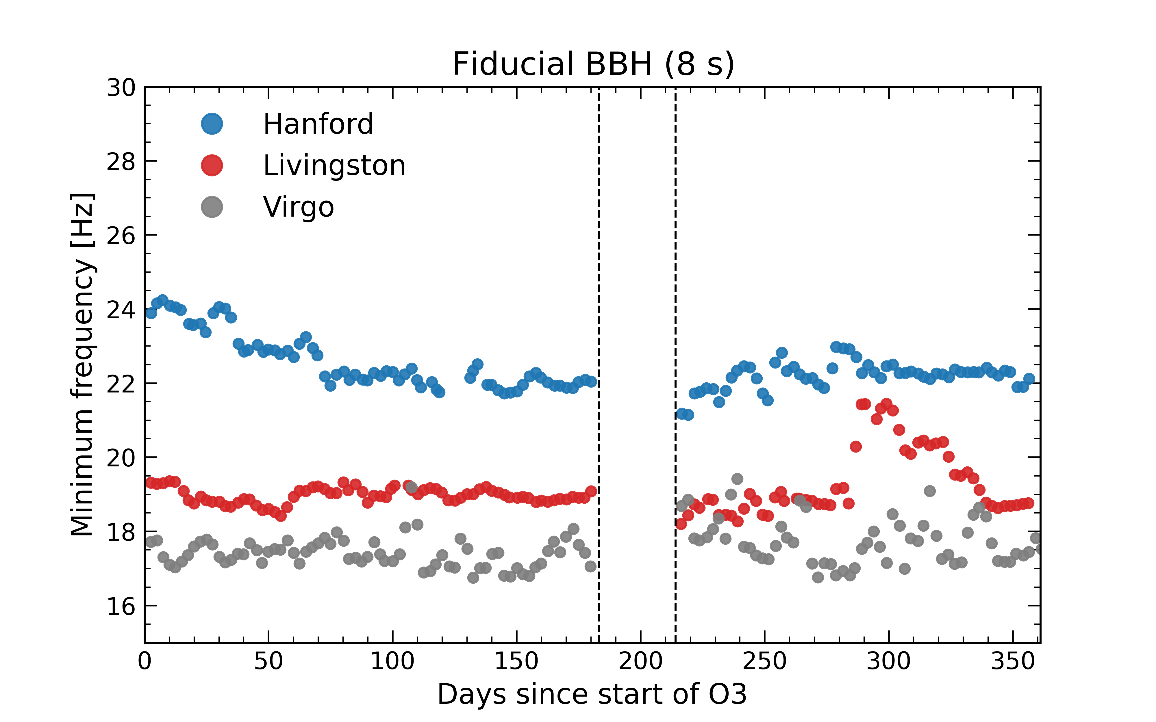
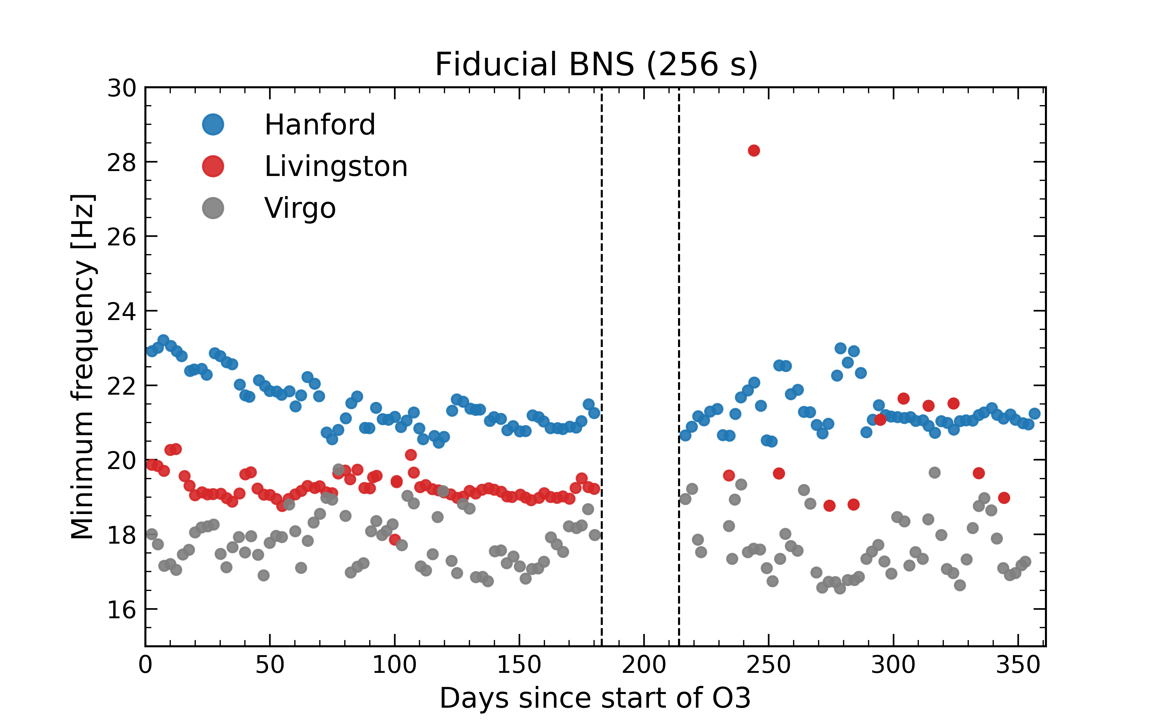
Figure 7: The estimated mean minimum frequency and 90% interval for LIGO Hanford (H1), LIGO Livingston (L1), and Virgo (V1) over the third observing run for the fiducial BBH (left panel) and fiducial BNS (right panel). To estimate the mean and interval, we apply a half-overlapping sliding window with a duration of 5 days. Dashed vertical lines mark the beginning and end of the A/B data collection periods.

VII Discussion

We have simulated gravitational wave signals from compact binary mergers to study the impact of the addition of Virgo and KAGRA on the ground-based detector network. We have focused on analyzing the improvements in the sky localization constraints for zero-spin binary black holes and neutron star binaries, and on the intrinsic source parameter estimates for high-spin aligned binary black holes. In Section III and IV, we have shown the results of the evolution of the sky-localization area for different detector networks when varying the binary neutron star sensitivity range of their least sensitive detector. Our results confirm that the addition of the Virgo and KAGRA detectors to the network comprising the two LIGO interferometers would improve the sky localization capabilities even when these additional detectors are not at their design sensitivity. Our findings expand on the results from several previous studies (Schutz, 2011; Fairhurst, 2011; Klimenko et al., 2011) that have focused on networks of equally sensitive detectors. Looking at the current sensitivities of ground-based interferometers, we find that the inclusion of Virgo into an HLV network is most beneficial starting from a Virgo sensitivity range of around 30–50 Mpc, corresponding to $\sim$1/5 of the sensitivity range of the LIGO detectors, that we fixed at 180 Mpc. These results, which depend on the specific position of the source relative to the Virgo detector and its inclination, are consistent with the relative sensitivity values of $\simeq 1/5-1/6$ that we computed in Section II. We find that our results also agree with the analysis of the binary black hole merger signal GW170814 (Abbott et al., 2017f). For this first clear three-detector observation, the 90% sky-localization area improves from 1160 to 60 deg² when adding the Virgo detector data, whose sensitivity range at the time was roughly 1/3 of the LIGO detector’s sensitivity. Although the source of GW170814 was much nearer than our simulated one, this is comparable to the improvement we see in Figure LABEL:fig:HLV_bbh for 60 Mpc, i.e., 10 deg² compared to the 800 deg² of the HL network.

A more general heuristic consideration is to look at the cumulative distribution of the antenna pattern function of the two individual LIGO detectors. When these are marginalized over all four angular parameters, one can notice that Virgo is almost exactly orthogonal to the LIGO detectors, as seen in Figure 3. So, it would have the same sensitivity as LIGO, or better, for about half of all the sources even if its sensitivity range was a factor of two smaller. Since we can argue that it would be enough to observe sources at about 1/3 of the LIGO signal-to-noise ratio in Virgo to still have meaningful parameter estimation, then Virgo would need to have at least a sensitivity a sixth that of LIGO, or $\simeq$30 Mpc average for about half of the sources. Comparing the field of view values of current optical telescopes, presented in Section I, with the results of our simulations, we notice that the Virgo detector would allow for an easier follow-up from 30 Mpc and 90 Mpc onwards, for the HLV and HV detector networks respectively, for a binary neutron star signal. In the non-spinning binary black hole case, the sky localization area is reduced to $\sim$10 deg² when Virgo is added to the HLV network with a sensitivity above 45 Mpc. For all the other two- and three-detector networks, despite the significant improvements in the localization constraints, these do never fall below the 10 deg² threshold. It is still noteworthy that the addition of KAGRA, with a sensitivity of 25 Mpc, into the HLK network reduces the inferred sky area from 200 deg² to 35 deg² for a binary neutron star source. From our four-detector network results, shown in Figure LABEL:fig:HLVK_bbh and LABEL:fig:HLVK_ns, we see that when Virgo has a sensitivity of 30 Mpc, 1/6 of LIGO’s, the addition of the KAGRA detector is still useful to constraint the sky-area of events maximizing KAGRA’s antenna pattern function. Specifically, for the binary neutron star case, the sky area can be constrained to under $\sim$35 deg² when KAGRA reaches a sensitivity greater than 20 Mpc, corresponding to $\sim$1/9 of LIGO’s. The mentioned results are obtained for a specific case, i.e., we consider a maximized Virgo antenna pattern function and a fixed distance, but our choice of parameters is a good approximation of the average values for the currently detectable population of sources (Abbott et al., 2023a). Furthermore, our focus on the ratios of relative detector sensitivities in a network easily allows for a translation of our results to future detector networks.

In our analysis, we also focused on two detector networks considering the variable duty factor the two LIGO detectors had in the previous observation runs, e.g., 65.3% and 61.8% during O2 for Hanford and Livingston, respectively (Abbott et al., 2018b). We found that even in the two detector cases, the addition of Virgo and KAGRA can have an important impact on the performance of the network. With Virgo, at a sensitivity of 100 Mpc or higher, we can expect the sky localization to be constrained to values smaller than the field view of current optical telescopes. This would highly increase our chances of detecting a multi-messenger event.

VIII Conclusion

We have run parameter estimation with Bilby on simulated gravitational wave signals from zero-spin black hole and neutron star binaries looking at the sky localization capability of different detector network configurations. We have focused on the improvements related to the addition of the Virgo and KAGRA detectors. We kept the sensitivity of the LIGO detectors fixed at 180 Mpc and varied the sensitivity of the additional detector. We found that the Virgo detector allows for the most significant improvements in the sky localization when it reaches a sensitivity that is approximately 1/6 that of the LIGO detectors. We expect a similar result for KAGRA, but we restrict our study to values up to 1/7 that of LIGO. Furthermore, we found that in the four-detector case, the addition of KAGRA would be beneficial at sensitivities above 1/10 that of the LIGO detectors, if Virgo is at 1/6 of the LIGO sensitivity.
We also simulated gravitational waves from high-spin aligned binary black holes and analyzed the improvements in the inference of the intrinsic source parameters with the sensitivity of the Virgo detector. We found the most significant improvements in the accuracy at sensitivities of the Virgo detector above half that of the LIGO detectors.
Finally, we have developed a tool to determine the optimal minimum frequency, defined as the lowest frequency for which the signal-to-noise ratio does increase by more than 0.1% with respect to higher cut-off frequency values. Testing this on O3 data by adding simulated gravitational wave signals, we found that 20 Hz is a good choice for the lower frequency cut-off in the parameter estimation analysis.

Finally, we have applied a naive scaling of the spectral density, but we have a good understanding of the noise budget of the detectors as a combination of power laws. In the future, we could use this knowledge to develop an interface to track the real-time changes in the PSD with the improvements in the detector. The parameters of interest would be the fitting constants for each power law in the PSD. This could allow us to overcome the imperfect scaling used in this work and would give us a deeper understanding of the connection between detector improvements and noise curves.

Appendix A Tables of simulation parameters and prior distributions

Table 2: Parameter values for simulated gravitational wave signals corresponding to non-spinning BBH, BNS, and high-spin BBH mergers. Values are given for the chirp mass ($\mathcal{M}$), mass ratio (q), luminosity distance (D_L), dimensionless spins (a₁ and a₂), tilt angles (tilt₁ and tilt₂), phase angles ($\phi_{12}$ and $\phi_{jl}$), angular parameter ($\theta_{jn}$), polarization angle ($\psi$), and overall phase. These simulated values serve as the ground truth for the simulated signals.

Parameter	BBH	BNS	High-spin BBH
$\mathcal{M}$	50	1.198	27.93
q	1	1	0.40
DL	2000	100	2000
a1	0	0	0.91
a2	0	0	0.94
tilt1	0	0	0
tilt2	0	0	0
$\phi_{12}$	0	0	0
$\phi_{jl}$	0	0	0
$\theta_{jn}$	0.4	0.4	0.4
$\psi$	2.66	2.66	2.66
$\phi$	1.3	1.3	1.3

Table 3: Prior distributions employed in the parameter estimation of simulated gravitational wave signals arising from high-spin and non-spinning BBH and BNS mergers. The symbol $\mathcal{U}$ denotes a uniform prior, and $\lambda^{2}$ represents a power law prior within the specified ranges. The table details the priors for chirp mass ($\mathcal{M}$), mass ratio (q), individual masses ($M_{1}$ and $M_{2}$), dimensionless spins ($\chi_{1}$ and $\chi_{2}$), tilt angles (tilt₁ and tilt₂), declination (DEC), luminosity distance (D_L), right ascension (RA), and various angle parameters..

Parameter	BBH	BNS	High-spin BBH
$\mathcal{M}$	$\mathcal{U}$ [25,60]	$\mathcal{U}$ [1.19799,1.19801]	$\mathcal{U}$ [15,60]
q	$\mathcal{U}$ [0.125,1]	$\mathcal{U}$ [0.125,1]	$\mathcal{U}$ [0.125,1]
M1	[1,100]	[1,100]	[5,100]
M2	[1,100]	[1,100]	[5,100]
$\chi_{1}$	$\mathcal{U}$ [0,0.99]	$\mathcal{U}$ [0,0.05]	-
$\chi_{2}$	$\mathcal{U}$ [0,0.99]	$\mathcal{U}$ [0,0.05]	-
$\mathrm{a}_{1}$	-	-	$\mathcal{U}$ [0,0.99]
$\mathrm{a}_{2}$	-	-	$\mathcal{U}$ [0,0.99]
tilt1	-	-	$\sin$
tilt2	-	-	$\sin$
$\phi_{12}$	-	-	$\mathcal{U}$ [0,2$\pi$]
$\phi_{jl}$	-	-	$\mathcal{U}$ [0,2$\pi$]
DL	$\lambda^{2}$ [10,10000]	$\lambda^{2}$ [10,500]	$\mathcal{U}$ [100,5000]
DEC	$\cos$	$\cos$	$\cos$
RA	$\mathcal{U}$ [0,2$\pi$]	$\mathcal{U}$ [0,2$\pi$]	$\mathcal{U}$ [0,2$\pi$]
$\theta_{jn}$	$\sin$	$\sin$	$\sin$
$\psi$	$\mathcal{U}$ [0,$\pi$]	$\mathcal{U}$ [0,$\pi$]	$\mathcal{U}$ [0,$\pi$]
$\phi$	$\mathcal{U}$ [0,2$\pi$]	$\mathcal{U}$ [0,2$\pi$]	$\mathcal{U}$ [0,2$\pi$]

Table 4: Setting employed for the dynesty sampler of Bilby for the parameter estimation of the simulated gravitational wave signals.

dynesty	nlive	npool	sample	naccept
zero-spin BBH/BNS	1000	30	acceptance-walk	60
high-spin BBH	2000	30	acceptance-walk	60

Appendix B Figures and table for the best network sky localization

	RA (rad)	DEC (rad)	PK	PV	PH	PL
HK Pbest	5.776	-0.952	0.62	0.17	0.72	0.32
HV Pbest	5.311	0.917	0.10	0.88	0.35	0.34
HLK Pbest	3.678	0.638	0.21	0.1	0.95	0.91
HLV Pbest	4.008	0.690	0.10	0.23	0.87	0.98
HLVK Pbest	3.873	0.529	0.20	0.20	0.85	0.98

Table 5: Table of the right ascension (RA), declination (DEC) and the values of the single detector’s antenna pattern amplitude for the source localization maximizing the combined antenna power pattern function, P_best, for each of the network configurations. The GPS time is fixed at 1379969683.0.

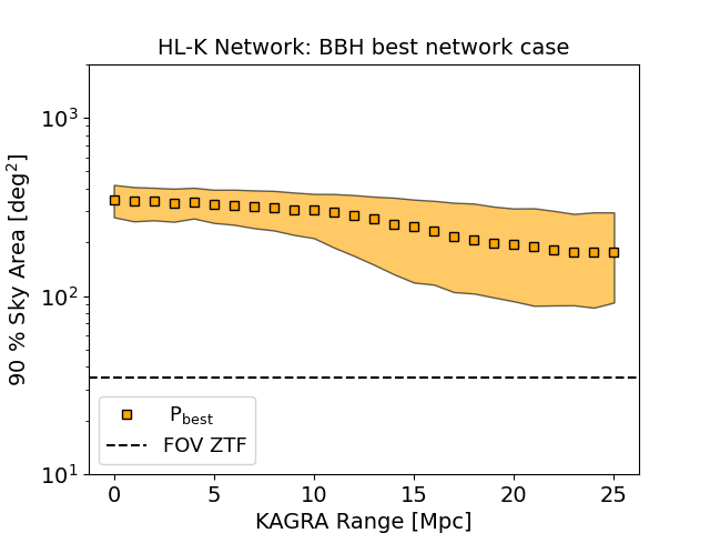
(a)

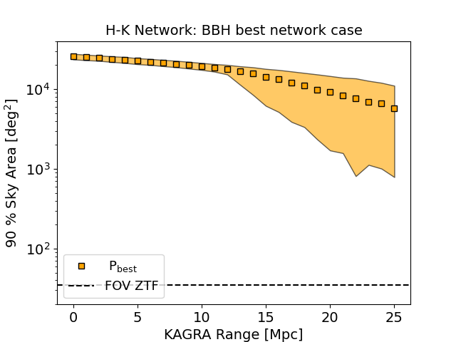
(b)

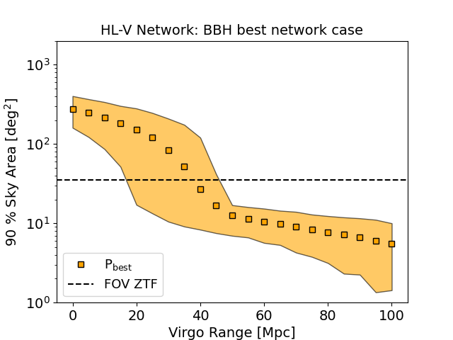
(c)

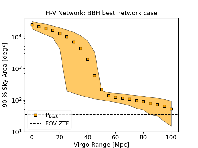
(d)

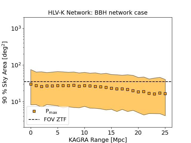
(e)

Figure 8: Zero-Spin Binary Black Hole Simulations
The mean and the 90 % probability contour of the sky area for varying detector range sensitivity values for a gravitational wave signal emitted by a binary black hole coalescence from the P_best source location for each detector network, orange points and area, respectively. The orange squares represent the mean value, and the areas stretch from the 5% to the 95% quantiles for each sensitivity range bin. The black dotted line corresponds to the field of view of the Zwicky Transient Facility. We obtained the 0 Mpc points from simulations excluding the least sensitive detector. We fixed the range sensitivity of the two LIGO detectors at 180 Mpc. (a): Varying the KAGRA detector and employing the LHK network. (b): Varying the KAGRA detector and employing the HLK network. (c): Varying the Virgo detector and employing the LHV network. (d): Varying the Virgo detector and employing the HLV network. (e): Varying the KAGRA detector and employing the LHVK network. Virgo’s sensitivity is fixed at 30 Mpc.

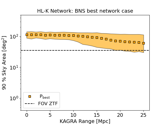
(a)

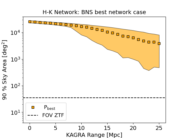
(b)

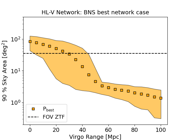
(c)

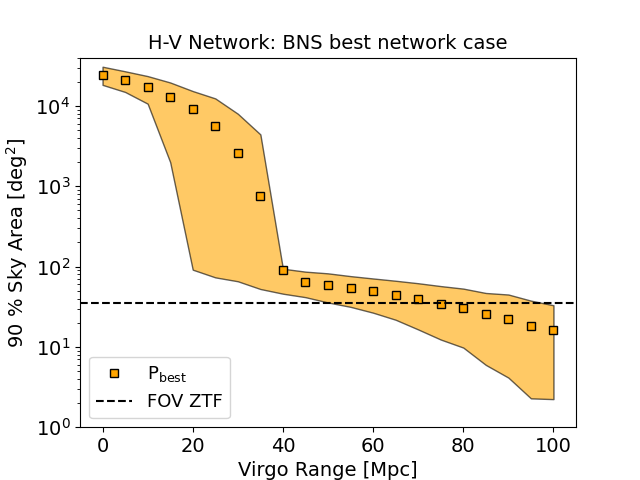
(d)

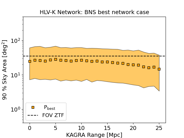
(e)

Figure 9: Binary Neutron Star Simulations
The mean and the 90% probability contour of the sky area for varying detector range sensitivity values for a gravitational wave signal emitted by a binary neutron star coalescence from the P_best source location for each detector network, orange dots and areas, respectively. The squares represent the mean value, and the areas stretch from the 5% to the 95% quantiles for each sensitivity range bin. The black dotted line corresponds to the field of view of the Zwicky Transient Facility. We obtained the 0 Mpc points from simulations excluding the least sensitive detector. We fixed the range sensitivity of the two LIGO detectors at 180 Mpc. (a): Varying the KAGRA detector and employing the LHK network. (b): Varying the KAGRA detector and employing the HLK network. (c): Varying the Virgo detector and employing the LHV network. (d): Varying the Virgo detector and employing the HLV network. (e): Varying the KAGRA detector and employing the LHVK network. Virgo’s sensitivity is fixed at 30 Mpc.