Seesaw Limit of the Nelson-Barr Mechanism
Abstract
We investigate how the solution to the strong CP problem and the explanation for the observed fermion mass hierarchies can be intrinsically related. Specifically, we explore the Nelson-Barr mechanism and identify its “seesaw limit”, where light quark masses are suppressed by large CP-violating terms. Upon adding three (two) vector-like quarks that mix with the down-type (up-type) quark sector of the Standard Model, we demonstrate how the lack of CP violation in the strong sector and the observed quark mass hierarchy can be simultaneously achieved.
I Introduction
The simplicity of the gauge sector of the Standard Model (SM) —only three parameters govern the interactions among its many fermions and gauge bosons— stems from the simplicity of the SM gauge group and, more generally, from the structure of gauge theories. In contrast, explaining the SM flavour sector requires at least 20 parameters once neutrino masses are included, and no underlying guiding principle is known. Our lack of understanding of the non-trivial hierarchies observed among the flavour parameters constitutes the so-called flavour puzzle Feruglio (2015).
Another well-known issue for which the SM does not offer a compelling explanation is the strong CP problem, i.e., the non-observation of CP violation in the strong interacting sector to a very high degree in spite of the possible presence of the effective phase breaking the symmetry. This becomes even more intriguing since receives a contribution from the flavour sector, more precisely from the quark Yukawa matrices, where CP is known to be violated.
The flavour puzzle may be addressed in many ways. For instance, the Froggatt-Nielsen mechanism Froggatt and Nielsen (1979) is a popular approach which explains hierarchical fermion masses from the distinctive interactions between fermions and flavons controlled by attributing different abelian flavour-dependent charges. Another approach, more successful for leptons, is to use properly broken flavour symmetries to explain the peculiar leptonic mixing pattern; see, e.g., Refs. Altarelli and Feruglio (2010); Feruglio and Romanino (2021) for a review. In particular, modular flavour symmetries Feruglio (2019) lead to very restrictive models.
Yet another appealing alternative is the implementation of seesaw scenarios, originally proposed to explain the smallness of neutrino masses Minkowski (1977); Yanagida (1979); Gell-Mann et al. (1979); Mohapatra and Senjanovic (1980); Schechter and Valle (1980), and later extended to charged lepton and quark masses Berezhiani (1985); Chang and Mohapatra (1987); Rajpoot (1987); Davidson and Wali (1987, 1988). Seesaw mechanisms for quarks generally occur in models where (i) new heavy quarks that mix with the SM quarks are introduced, and (ii) the conventional Yukawa interactions between the SM quarks and Higgs are forbidden by symmetries, e.g., in left-right Chang and Mohapatra (1987); Rajpoot (1987); Davidson and Wali (1987, 1988), 3-3-1 Dias et al. (2020, 2022) and Jana et al. (2022); Chen and Gu (2023) extensions of the SM. The large masses of the extra quarks are responsible for suppressing the SM quark masses with respect to the electroweak scale as well as providing small mixing between the SM and the heavy quarks. The presence of extra quarks that mix with the SM fields, such as the seesaw-mediating ones, leads to rich phenomenology. If sufficiently light, they can be abundantly produced and subsequently decay at colliders due to their interactions with SM gauge bosons. Additionally, their mixing with the SM quarks induces flavour-violating interactions as well as departures from unitarity in the quark mixing, Cabibbo-Kobayashi-Maskawa (CKM), matrix. These phenomena offer multiple experimental opportunities to probe the masses and mixing of the extra quarks; for a summary of relevant constraints see Alves et al. (2024).
Regarding the strong CP problem, the Peccei-Quinn (PQ) Peccei and Quinn (1977a, b) and the Nelson-Barr Nelson (1984); Barr (1984) mechanisms provide two fundamentally distinct yet effective solutions. In the Nelson-Barr scheme, one assumes that CP is a fundamental symmetry of nature that is spontaneously broken, and the couplings of the SM to the CP breaking sector are arranged to guarantee vanishing at tree level. The challenge is to generate an order one CKM phase and, simultaneously, suppress corrections to sufficiently. Corrections may already show up at one-loop Bento et al. (1991), although it may be postponed to two-loops by using a nonconventional CP symmetry Cherchiglia and Nishi (2019). Quite similarly to the axion solution, the Nelson-Barr solution also suffers from a quality problem Dine and Draper (2015); Asadi et al. (2023); Choi et al. (1993), which can be ameliorated by additional gauge symmetries Asadi et al. (2023), supersymmetry Dine and Draper (2015) or strong dynamics Valenti and Vecchi (2021a).
In Nelson-Barr settings, the spontaneous breaking of CP is transmitted to the SM through the mixing of SM quarks with heavy vector-like quarks of Nelson-Barr type (NB-VLQs) Cherchiglia and Nishi (2020); Cherchiglia et al. (2021); Alves et al. (2023); Valenti and Vecchi (2021b). The NB-VLQs that mediate the CP breaking may lie at much lower energies, only constrained to be above the TeV scale from collider searches. To comply with the Barr criteria Barr (1984), the NB-VLQs can only be electroweak singlets or doublets, in the same representations of SM quarks. The case of doublets was argued to lead to too large corrections to Vecchi (2017). For singlets, we have found for one Cherchiglia and Nishi (2020); Cherchiglia et al. (2021) or two Alves et al. (2023) NB-VLQs that they typically couple to the SM quarks and Higgs following the hierarchy of the CKM last row or column, a feature that alleviates the strongest flavour constraints that apply to the first two quark families. For special points for one NB-VLQ, one can even switch off the coupling of such a heavy quark with a given quark flavour Alves et al. (2023); Cherchiglia et al. (2022).
Several connections between the strong CP and the fermion mass hierarchy problems have been explored in the literature. There are proposals with extra quarks getting massive at the PQ scale and leading to seesaw-suppressed masses for all the standard quarks Kang and Shin (1986), or tree-level (seesaw) and loop-suppressed masses for the different generations Babu and He (1989). Interrelated solutions to these problems have also been investigated in SM gauge extensions featuring the PQ mechanism, such as a 3-3-1 model Dias et al. (2018) and a non-universal model Garnica et al. (2021). Furthermore, the phase can be generated at the two-loop level in extended left-right models incorporating seesaw mechanisms for the SM fermions Babu and Mohapatra (1989, 1990). On the other hand, the Froggat-Nielsen and the Peccei-Quinn mechanisms can be realised synergistically by identifying the Froggat-Nielsen flavon with the PQ axion Ema et al. (2017).
In this work, we propose a new framework where solutions to both the strong CP problem and the flavour puzzle are also directly linked. We focus on the Nelson-Barr solution to the strong CP problem and explore the possibility that the newly introduced VLQs generate seesaw-suppressed masses for the SM quarks.
The outline of this article is the following: In Sec. II, we present an overview of the NB-VLQs that transmit CP violation to the SM in the Nelson-Barr mechanism. The “seesaw limit” of the Nelson-Barr mechanism is identified and important relations are derived in Sec. III. In the following section, Sec. IV, we study a scenario where three down-type vector-like quarks are added to the SM while in Sec. V, we explore the consequences of the SM extended by two up-type vector-like quarks. Finally, our conclusions are summarised in Sec. VI.
II The Nelson-Barr mechanism
In this section, we provide an overview of the so-called Nelson-Barr mechanism Nelson (1984); Barr (1984), which tackles the strong CP problem via the spontaneous breaking of the CP symmetry. For simplicity and clarity, we focus here on the case in which only the down-type quark sector of the SM is extended. Similar steps can be followed when extending the up-type or both quark sectors instead. We start by introducing a set of vector-like quarks (VLQs) transforming under the SM symmetry group, , as
| (1) |
In addition to , two discrete symmetries, and , are imposed. Under the latter, only the new quarks transform non-trivially.
Given these ingredients, the Yukawa interactions for the quarks can then be written as
| (2) |
with the last term, which softly breaks as well as , arising from spontaneous symmetry breaking when scalar fields – singlets under – acquire non-trivial complex vevs111For instance, we can have , where are () real matrices and .. All the other terms are assumed to conserve (as well as ), implying that and – both – as well as – – are real matrices. Once the Higgs doublet acquires a vev, , we can write down the following mass matrix for the down-type quarks,222Note that in generic settings some zeros may be produced by weak basis changes; see a discussion in Ref. Alves et al. (2024). Here, due to the softly broken and symmetries, this structure with real entries cannot result from a weak basis change.
| (3) |
whereas for the up-type quarks, we have , which is taken diagonal for simplicity.
The contributions at tree level to coming from the quark sector () vanish because . Moreover, since the symmetry is only broken (spontaneously) through , the bare term also vanishes. Consequently, the effective parameter vanishes at tree level.
It is convenient to perform a unitary transformation on the right-handed fields , so that becomes Alves et al. (2023, 2024)
| (4) |
where
| (5) |
These mass matrices are then related via
| (6) | ||||
with
| (7) |
In addition, by using the relation , we see that the Yukawa coupling of the heavy quarks and Yukawa coupling of the SM quarks obey an interesting relation Cherchiglia and Nishi (2020); Alves et al. (2023):
| (8) |
It follows that roughly follows the hierarchy of the CKM entries.
Coming back to in Eq. (3), we notice that the terms and conserve the SM symmetry structure, and, as such, we can safely assume that they emerge at much higher energy scales than , which simply translates into
| (9) |
In this case, we can block diagonalise via the unitary transformation on the left-handed fields
| (10) |
where is a function of following the same ansatz for in Eq. (5). At leading order, we obtain
| (11) | |||||
| (12) | |||||
Finally, by further diagonalising by means of a unitary transformation, we find the (squared) masses of the heavy, non-standard quarks. On the other hand, is approximately diagonalised by the CKM matrix so that , where are the masses of the down, strange and bottom quarks, respectively. For up-type VLQs, we should replace .
III The seesaw limit of the Nelson-Barr mechanism
We now explore the seesaw limit of the model described in the previous section. For simplicity, we first assume that the vector-like quarks appear in the same number as the standard quarks, i.e. . In this case, the down-type quark mass matrix in Eq. (3) becomes333Notice that by swapping the first and second block columns, which is equivalent to a change of basis, the resulting matrix has a type-I Dirac-seesaw texture
| (13) |
The seesaw limit consists in the special case of the condition Eq. (9) in which 444We distinguish between the condition Eq. (9) for the validity of the seesaw approximation for the mixing of the left-handed fields and this subcase where the term that softly breaks CP is dominant.
| (14) |
This limit allows for the expansion of in Eq. (11) as
| (15) | ||||
where the last step is only possible when is a square matrix, while the second line is only possible for . Substituting this result back into Eq. (11), we obtain
| (16) |
Therefore, we find that the standard quark masses are seesaw suppressed with respect to the electroweak scale by a factor
| (17) |
which has entries much smaller than unity. This quantity is simply in the notation of Ref. Alves et al. (2023).
If, for instance, we assume that , then the quark masses are roughly given by . Thus, instead of being proportional to GeV, down-type quark masses are now proportional to an effective scale GeV. Consequently, the CP-conserving Yukawa entries in can be two orders of magnitude larger than the ones in the Standard Model.
Furthermore, to study the physical cases consistent with the current quark mixing picture, it is convenient to solve Eq. (16) for in terms of the other matrices as
| (18) |
where is the diagonal Yukawa coupling matrix for the down-type quarks in the SM, and is a generic unitary matrix. This inversion is particularly simple in the seesaw limit; away from this limit a more complicated parametrization similar to the ones in Refs. Cherchiglia and Nishi (2020); Alves et al. (2023) will be needed. Without loss of generality, we can choose a basis in which is diagonal and , with orthogonal and diagonal . Finally, we can see that if has order-one entries, is larger than by, at least, . This is clear if we substitute Eq. (18) into Eq. (17), obtaining
| (19) |
Note that is the CKM matrix of the SM with two additional phases Cherchiglia and Nishi (2020):
| (20) |
where is, e.g., the standard parametrization. These additional phases arise because the Yukawa in Eq. (6) loses rephasing freedom from the left to keep real.
Turning to the heavy quarks, at leading order, their mass matrix is given by
| (21) |
In the seesaw limit, this mass matrix is dominated by which can be related to by
| (22) |
Additionally, the leading contribution to the mixing parameter in Eq. (11) is given by
| (23) |
Finally, the relation (8) becomes
| (24) |
This relation now indicates that is larger than the SM Yukawa by the factor .
Special cases: , incomplete seesaw
The case presented above assumes the introduction of a vector-like quark per standard quark generation, i.e., . As a result, the seesaw mechanism suppresses the overall mass scale for all the standard quarks. Nevertheless, the seesaw limit is of interest even in cases with fewer vector-like quarks, . This is particularly true for the up-type sector, as we will discuss in Sec. V.
In scenarios with fewer vector-like quarks than standard ones (), the matrix is not square and, as such, the approximation in Eq. (LABEL:eq:wexp) is only valid up to the second to last line, i.e.,
| (25) | ||||
Thus, in contrast with the case where , not all standard quark masses, obtained from Eq. (11) with Eq. (25), become suppressed. In this case, only of the standard quarks get seesaw-suppressed masses, while the remaining masses remain proportional to the Higgs vev .
To understand this, notice that the first term in Eq. (25), that is, the matrix has rank with the non-vanishing eigenvalues equal to unity, since it is a projection matrix obeying and is rank . Therefore, taking, for instance, and rotating the fields to a basis where is diagonal, we have
| (26) |
where represents the seesaw suppressed terms in – the (rotated) second term in Eq. (25). As , cf. Eq. (11), for a with similar entries, two of the quark masses are seesaw suppressed, while one remains non-suppressed. Similarly, when , one quark mass becomes seesaw suppressed and the other two do not.
In such cases, instead of Eq. (18), we can use the formulae derived in Refs. Cherchiglia and Nishi (2020); Alves et al. (2023) to find benchmarks satisfying the current quark mixing picture. The exact parametrization involves solving the first equation of (11) for . To that end, we first rewrite it as
| (27) |
If we split in terms of its real and imaginary parts, we can solve the real part of (27) by
| (28) |
where is a real orthogonal matrix to be determined from the imaginary part of (27), i.e.,
| (29) |
By choosing an appropriate basis for , a parametrization can be found for Cherchiglia and Nishi (2020) and Alves et al. (2023). For the latter, additional parameters are necessary to describe and .
IV Nelson-Barr seesaw for the down-type quarks
We now discuss in more detail the consequences of having three down-type VLQs participating in the Nelson-Barr mechanism as introduced in Sec. III. We generate points by using Eq. (18) in the basis where
| (30) |
where is a real orthogonal matrix, and is the diagonal matrix of singular values. In the analyses that follow, we vary the diagonal entries of in the range GeV and , where are the three angles that parametrise . The SM quark masses and CKM matrix parameters are fixed to their best-fit values Workman et al. (2022). Furthermore, we take into account bounds from VLQ searches Aad et al. (2012) to filter out solutions with one or more VLQs lighter than TeV.
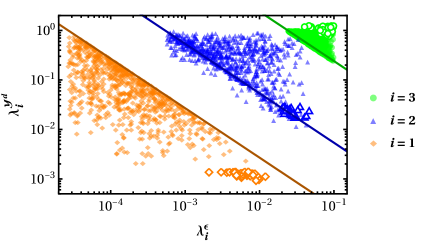
Let us first analyze our seesaw expansion matrix in Eq. (17) which is the ratio between the CP-conserving bare VLQ mass and the dominant CP-violating contribution. In the seesaw limit, this matrix should be naturally small as it gives in Eq. (16) the suppression of to generate the SM down quark masses. Another expression of this feature can be seen in Eq. (19). To ensure that the seesaw limit, see Eq. (14), is satisfied by all of our solutions, we select points for which all of the singular values of are at least one order of magnitude larger than the singular values of or, equivalently, all of the eigenvalues of are at least one order of magnitude larger than those of . This suppression can be seen in Fig. 1 where we show the singular values of as a function of the singular values of . In the plot, we denote as each singular value of the matrix in increasing order. The filled and hollow symbols denote two sets of points:
| Generic (filled): | (31) | |||
| Hierarchical (hollow): |
In the second case, the singular values follow the hierarchy of the SM Yukawas allowing for a variation of 25%. We can see in the figure in the generic set that of the same order requires hierarchical to account for the hierarchy of the SM Yukawa . On the other hand, as becomes hierarchical, a less hierarchical is necessary. In the extreme case of following the hierarchy of the SM Yukawa (hierarchical set), non-hierarchical values for are allowed.
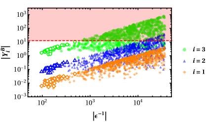
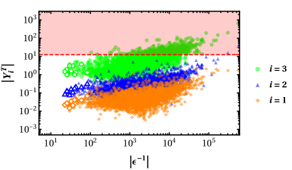
We can now illustrate the behaviour of the Yukawa couplings , cf. Eq. (24), of the heavy quark to the SM Higgs and quark . Instead of the individual couplings, we take the norm of the couplings to each SM family:
| (32) |
In Fig. 2 we show this norm of Yukawas as a function of the norm of :
| (33) |
We can see that the rough hierarchy follows
| (34) |
analogous to the case of one or two VLQs Cherchiglia and Nishi (2020); Alves et al. (2023). We also observe that generic has larger Yukawas and larger while the hierarchical case has smaller Yukawas and smaller in accordance to Eq. (24). For the former set, many points are excluded by the perturbativity constraint which is shaded red.
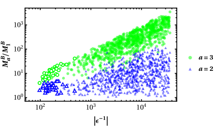
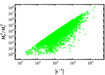
Finally, we show in Fig. 3 the ratio of the heavy masses in Eq. (21) compared to their lightest mass as a function of . In accordance with Eq. (22), we see that larger tends to lead to a larger hierarchy among the heavy quarks. For the hierarchical set where the entries of are all of the same order, the heavy masses are also non-hierarchical.
V Nelson-Barr seesaw for the up-type quarks
We now turn to the up-type quarks. Since the top Yukawa is already of order one, we aim to provide an explanation for the observed hierarchy among up and charm quarks only. This can be achieved by introducing two NB-VLQs. In this case, we cannot use Eq. (18) since it was derived under the assumption that is invertible (it is a matrix now)555For up-type quarks, instead of and , vector-like and standard quarks are denoted by and , respectively.. We instead rely on a parametrization devised in Cherchiglia and Nishi (2020); Alves et al. (2023), which takes the known up-type quark masses, CKM mixing and the lightest VLQ mass as inputs (among other non-physical variables). We fixed the SM quantities to their best-fit values Workman et al. (2022), the lightest VLQ mass to 1.3 TeV Alves et al. (2024) while the other parameters were varied in a broad range. Notice that is a derived quantity in this framework, cf. (28). In order to consider the seesaw regime, we filtered the points for which the singular values of are at least one order of magnitude larger than those of . Moreover, we also applied a filter for perturbativity, allowing only points for which . We should notice that, for 2 NB-VLQs, Eq. (17) is not defined, while is. Thus, to make contact with the plots of the previous section, we will define as the inverse of the singular values of .
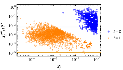
In figure 4, we show the ratio among the two smallest singular values of to the third, against . As the ratio approaches the SM value (orange line), the singular values of are at most one order of magnitude apart. In this regime, the observed hierarchy among the first and second family masses comes from the hierarchical structure of . On the other hand, as the singular values of differ by roughly 3 orders of magnitude (which is the observed hierarchy among the first and second up-quark family in the SM), the ratios , approach similar values. More precisely, they are close to the blue line, which represents the ratio . In this case, the observed hierarchy among up and charm quark masses resides in . In the figure, the hollow points comply with .
In figure 5, we show how the norm () varies in terms of the norm of , while in figure 6 we illustrate the dependence of the ratio between the two VLQ masses in the same quantity. For comparison against the plots of the previous section, we added points that violate perturbativity in these figures. We notice that, for , all green points are excluded setting an upper bound on this quantity. Since the hollow points comply with , we see that if the hierarchy between the first and second up-quarks family resides in , the norm of attains its lowest values. Similar patterns occur in the case of 3 VLQs.
VI Conclusions
Although the SM is very successful in explaining a plethora of phenomena, there are still some puzzling issues, such as the strong CP problem and the observed fermion mass hierarchies, to cite a few. In this work, seeking a common solution to these problems, we have identified and investigated the “seesaw limit” of the Nelson-Barr mechanism. We have studied in detail how the introduction of three heavy VLQs, that mix with the Standard Model fields, can provide a natural mechanism to suppress the SM down quark masses in relation to the EW scale. In particular, we have seen that the source of CP violation in the quark sector, i.e., the SM-VLQ-mixing term in Eqs. (2) and (3), is also behind the seesaw suppression of light quark masses. Since these VLQs are connected to the Nelson-Barr mechanism, not only the strong CP problem can be addressed, but also the couplings between them and the standard quarks are typically hierarchical. This in turn allows our model to naturally evade strong bounds from flavour observables coming from first and second quark families. We have also shown in a similar model with two up-type VLQs that the hierarchy among the SM up quarks can be partly explained by the hierarchy of the small seesaw parameters.
Acknowledgements.
This research was partially supported by the Conselho Nacional de Desenvolvimento Científico e Tecnológico (CNPq), by grants 308280/2023-7 (A.G.D.), 312866/2022-4 (C.C.N.), and 166523/2020-8 (A.L.C.). Financial support by Fundação de Amparo à Pesquisa do Estado de São Paulo (FAPESP) is also acknowledged under the grant 2014/19164-6 (C.C.N.). J.L. is supported by the Spanish grants PID2020-113775GB-I00 (AEI/10.13039/501100011033) and Prometeo CIPROM/2021/054 (Generalitat Valenciana). A.L.C is supported by a postdoctoral fellowship from the Postdoctoral Researcher Program - Resolution GR/Unicamp No. 33/2023.References
- Feruglio (2015) F. Feruglio, Eur. Phys. J. C 75, 373 (2015), arXiv:1503.04071 [hep-ph] .
- Froggatt and Nielsen (1979) C. D. Froggatt and H. B. Nielsen, Nucl. Phys. B 147, 277 (1979).
- Altarelli and Feruglio (2010) G. Altarelli and F. Feruglio, Rev. Mod. Phys. 82, 2701 (2010), arXiv:1002.0211 [hep-ph] .
- Feruglio and Romanino (2021) F. Feruglio and A. Romanino, Rev. Mod. Phys. 93, 015007 (2021), arXiv:1912.06028 [hep-ph] .
- Feruglio (2019) F. Feruglio, “Are neutrino masses modular forms?” in From My Vast Repertoire …: Guido Altarelli’s Legacy, edited by A. Levy, S. Forte, and G. Ridolfi (2019) pp. 227–266, arXiv:1706.08749 [hep-ph] .
- Minkowski (1977) P. Minkowski, Phys. Lett. 67B, 421 (1977).
- Yanagida (1979) T. Yanagida, Conf. Proc. C7902131, 95 (1979).
- Gell-Mann et al. (1979) M. Gell-Mann, P. Ramond, and R. Slansky, Conf. Proc. C 790927, 315 (1979), arXiv:1306.4669 [hep-th] .
- Mohapatra and Senjanovic (1980) R. N. Mohapatra and G. Senjanovic, Phys. Rev. Lett. 44, 912 (1980).
- Schechter and Valle (1980) J. Schechter and J. W. F. Valle, Phys. Rev. D 22, 2227 (1980).
- Berezhiani (1985) Z. G. Berezhiani, Phys. Lett. B 150, 177 (1985).
- Chang and Mohapatra (1987) D. Chang and R. N. Mohapatra, Phys. Rev. Lett. 58, 1600 (1987).
- Rajpoot (1987) S. Rajpoot, Phys. Lett. B 191, 122 (1987).
- Davidson and Wali (1987) A. Davidson and K. C. Wali, Phys. Rev. Lett. 59, 393 (1987).
- Davidson and Wali (1988) A. Davidson and K. C. Wali, Phys. Rev. Lett. 60, 1813 (1988).
- Dias et al. (2020) A. G. Dias, J. Leite, B. L. Sánchez-Vega, and W. C. Vieira, Phys. Rev. D 102, 015021 (2020), arXiv:2005.00556 [hep-ph] .
- Dias et al. (2022) A. G. Dias, J. Leite, and B. L. Sánchez-Vega, Phys. Rev. D 106, 115008 (2022), arXiv:2207.06276 [hep-ph] .
- Jana et al. (2022) S. Jana, S. Klett, and M. Lindner, Phys. Rev. D 105, 115015 (2022), arXiv:2112.09155 [hep-ph] .
- Chen and Gu (2023) S.-P. Chen and P.-H. Gu, Nucl. Phys. B 986, 116057 (2023), arXiv:2211.01906 [hep-ph] .
- Alves et al. (2024) J. a. M. Alves, G. C. Branco, A. L. Cherchiglia, C. C. Nishi, J. T. Penedo, P. M. F. Pereira, M. N. Rebelo, and J. I. Silva-Marcos, Phys. Rept. 1057, 1 (2024), arXiv:2304.10561 [hep-ph] .
- Peccei and Quinn (1977a) R. D. Peccei and H. R. Quinn, Phys. Rev. Lett. 38, 1440 (1977a), [,328(1977)].
- Peccei and Quinn (1977b) R. D. Peccei and H. R. Quinn, Phys. Rev. D 16, 1791 (1977b).
- Nelson (1984) A. E. Nelson, Phys. Lett. B 136, 387 (1984).
- Barr (1984) S. M. Barr, Phys. Rev. Lett. 53, 329 (1984).
- Bento et al. (1991) L. Bento, G. C. Branco, and P. A. Parada, Phys. Lett. B 267, 95 (1991).
- Cherchiglia and Nishi (2019) A. L. Cherchiglia and C. C. Nishi, JHEP 03, 040 (2019), arXiv:1901.02024 [hep-ph] .
- Dine and Draper (2015) M. Dine and P. Draper, JHEP 08, 132 (2015), arXiv:1506.05433 [hep-ph] .
- Asadi et al. (2023) P. Asadi, S. Homiller, Q. Lu, and M. Reece, Phys. Rev. D 107, 115012 (2023), arXiv:2212.03882 [hep-ph] .
- Choi et al. (1993) K.-w. Choi, D. B. Kaplan, and A. E. Nelson, Nucl. Phys. B 391, 515 (1993), arXiv:hep-ph/9205202 .
- Valenti and Vecchi (2021a) A. Valenti and L. Vecchi, JHEP 07, 152 (2021a), arXiv:2106.09108 [hep-ph] .
- Cherchiglia and Nishi (2020) A. L. Cherchiglia and C. C. Nishi, JHEP 08, 104 (2020), arXiv:2004.11318 [hep-ph] .
- Cherchiglia et al. (2021) A. L. Cherchiglia, G. De Conto, and C. C. Nishi, JHEP 11, 093 (2021), arXiv:2103.04798 [hep-ph] .
- Alves et al. (2023) G. H. S. Alves, A. L. Cherchiglia, and C. C. Nishi, Phys. Rev. D 108, 035049 (2023), arXiv:2304.06078 [hep-ph] .
- Valenti and Vecchi (2021b) A. Valenti and L. Vecchi, JHEP 07, 203 (2021b), arXiv:2105.09122 [hep-ph] .
- Vecchi (2017) L. Vecchi, JHEP 04, 149 (2017), arXiv:1412.3805 [hep-ph] .
- Cherchiglia et al. (2022) A. L. Cherchiglia, G. De Conto, and C. C. Nishi, JHEP 03, 010 (2022), arXiv:2112.03943 [hep-ph] .
- Kang and Shin (1986) K. Kang and M. Shin, Phys. Rev. D 33, 2688 (1986).
- Babu and He (1989) K. S. Babu and X.-G. He, Phys. Lett. B 219, 342 (1989).
- Dias et al. (2018) A. G. Dias, J. Leite, D. D. Lopes, and C. C. Nishi, Phys. Rev. D 98, 115017 (2018), arXiv:1810.01893 [hep-ph] .
- Garnica et al. (2021) Y. A. Garnica, S. F. Mantilla, R. Martinez, and H. Vargas, J. Phys. G 48, 095002 (2021), arXiv:1911.05923 [hep-ph] .
- Babu and Mohapatra (1989) K. S. Babu and R. N. Mohapatra, Phys. Rev. Lett. 62, 1079 (1989).
- Babu and Mohapatra (1990) K. S. Babu and R. N. Mohapatra, Phys. Rev. D 41, 1286 (1990).
- Ema et al. (2017) Y. Ema, K. Hamaguchi, T. Moroi, and K. Nakayama, JHEP 01, 096 (2017), arXiv:1612.05492 [hep-ph] .
- Workman et al. (2022) R. L. Workman et al. (Particle Data Group), PTEP 2022, 083C01 (2022).
- Aad et al. (2012) G. Aad et al. (ATLAS), Phys. Lett. B 712, 22 (2012), arXiv:1112.5755 [hep-ex] .