Synchronization-induced violation of thermodynamic uncertainty relations

Abstract

Fluctuations affect the functionality of nanodevices. Thermodynamic uncertainty relations (TURs), derived within the framework of stochastic thermodynamics, show that a minimal amount of dissipation is required to obtain a given relative energy current dispersion, that is, current precision has a thermodynamic cost. It is therefore of great interest to explore the possibility that TURs are violated, particularly for quantum systems, leading to accurate currents at lower cost. Here, we show that two quantum harmonic oscillators are synchronized by coupling to a common thermal environment, at strong dissipation and low temperature. In this regime, periodically modulated couplings to a second thermal reservoir, breaking time-reversal symmetry and taking advantage of non-Markovianity of this latter reservoir, lead to strong violation of TURs for local work currents, while maintaining finite output power. Our results pave the way for the use of synchronization in the thermodynamics of precision.

I Introduction

In 1665 Huygens observed the synchronization of two pendulum clocks mounted on a common support [1]. Since then, synchronization has emerged as a universal concept in the theory of dynamical systems, with a broad range of applications in fields ranging from science and engineering to social life [2]. More recently, the phenomenon has been investigated and characterized in quantum systems [3, 4, 5, 6, 7, 8, 9, 10, 11, 12, 13, 14, 15, 16, 17] with, however, only a few studies addressing thermodynamic signatures of synchronization  [18, 19]. Just as thermodynamics started in the 1800s spurred by the industrial revolution, in the same way the miniaturization of devices, and in particular the emergence of new quantum technologies, pushes the field of thermodynamics into new applied and fundamental challenges [20, 21, 22, 23, 24, 25, 26]. In the thermodynamics of small (quantum) systems, fluctuations [27, 28, 29] play a prominent role, and thermodynamic uncertainty relations (TURs), derived within the framework of classical stochastic thermodynamics, establish a lower bound to the amount of dissipation needed to reduce relative energy current fluctuations to a given level [30, 32, 33, 31, 34, 35, 36, 37, 38, 39, 40]. This seminal result motivated the quest for possible mechanisms to violate TURs, and consequently reduce the thermodynamic cost of precision. Routes for TUR violations include breaking of time-reversal symmetry (TRS) [42, 43, 41] and quantum coherences [44, 47, 45, 46, 48, 49, 50, 51, 52, 53, 54, 55, 56, 57, 58, 59]. Although it might be intuitive that synchronization, by locking the relative motion of system constituents, can reduce fluctuations, its possible role in TURs violation has not yet been explored.

In this work, we consider two quantum harmonic oscillators (QHOs) coupled to common thermal baths (see Fig. 1 for a schematic drawing of our model). The couplings to one bath are static and induce not only dissipation but also the emergence of correlations between the two otherwise independent oscillators. At strong damping and low temperatures, the oscillators are synchronized, oscillating at a common frequency and in phase opposition. The oscillators are then in contact with a second thermal bath, with periodically driven couplings breaking TRS. In the synchronization regime, the TURs for the local work currents, i.e., the injected or extracted power of each oscillator, can be strongly violated, despite the fact that the TUR for total power is rigorously proven as never violated. In addition, the finite cutoff frequency for the dynamically coupled bath spectral density, which generally implies non-Markovian effects [60, 61, 62], allows local TURs to be violated in the fast driving diabatic regime. In this regime, the violation of TUR is accompanied by the possibility of extracting finite and sizeable power from one oscillator. These results, already present in a isothermal regime, can benefit from the presence of a temperature gradient, especially in the non-linear regime where TUR violation is achieved in a wide parameter region.

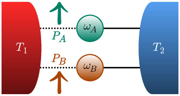
Figure 1: Sketch of the dynamical quantum thermal machine. Two quantum harmonic oscillators, with frequencies $\omega_{A}$ and $\omega_{B}$, are in contact with two common thermal reservoirs at temperatures $T_{\nu}$, with $\nu=1,2$. Power $P_{l}$ can be injected or extracted from the $l=A,B$ subsystem, while heat currents $J_{\nu}$ flow from or toward the reservoirs. External monochromatic drives modulate the weak coupling with the $\nu=1$ reservoir, while the coupling with $\nu=2$ is static and much stronger, and it is responsible for synchronization.

II Results

II.1 General setting

Two uncoupled (no direct coupling) quantum harmonic oscillators ($l=A,B$) in contact with two common thermal reservoirs ($\nu=1,2$) are the subsystems constituting the working medium (WM) of the quantum thermal machine under study, as sketched in Fig. 1. The total Hamiltonian is (we set $\hbar=k_{B}=1$)

$$H^{(t)}=\sum_{l=A,B}H_{l}+\sum_{\nu=1,2}\big{[}H_{\nu}+H_{{\rm int},\nu}^{(t)}\big{]}~{},$$ (1)

with $H_{l}=\frac{p_{l}^{2}}{2m}+\frac{1}{2}m\omega_{l}^{2}x_{l}^{2}$ the Hamiltonian of the $l$-th QHO (same mass $m$ but different characteristic frequencies $\omega_{A}$ and $\omega_{B}$). The reservoirs $H_{\nu}$ are modelled with the Caldeira-Leggett approach of quantum dissipative systems [63, 64, 65, 66] as a collection of independent harmonic oscillators, while the system-reservoir interaction $H_{{\rm int},\nu}^{(t)}=\sum_{l=A,B}H_{{\rm int},\nu,l}^{(t)}$ is a bilinear coupling $\sim x_{l}\sum_{k=1}^{+\infty}g^{(l)}_{\nu}(t)c_{k,\nu}X_{k,\nu}$ in the subsystem $x_{l}$ and bath $X_{k,\nu}$ position operators, where $c_{k,\nu}$ describe the coupling strengths weighted by the modulating function $g^{(l)}_{\nu}(t)$ (see Appendix A for details). We assume that the couplings with the $\nu=1$ reservoir are weak and oscillate in time [67, 68, 69, 70], with two independent monochromatic drives of the form

$$g_{1}^{(A)}(t)=\cos(\Omega t)~{},\quad g_{1}^{(B)}(t)=\cos(\Omega t+\phi)~{},$$ (2)

with $\Omega$ the external frequency and $\phi$ a relative phase. The couplings with the $\nu=2$ reservoir, instead, are static, $g_{2}^{(l)}=1$. Furthermore, the couplings with the $\nu=2$ bath are stronger than those with the $\nu=1$ bath.

The properties of the $\nu$-th bath, including possible memory effects and non-Markovian behaviour [71, 72, 73, 74, 75], are governed by the so-called spectral density [64] ${\cal J}_{\nu}(\omega)\equiv\frac{\pi}{2}\sum_{k=1}^{+\infty}\frac{c^{2}_{k,\nu}}{m_{k,\nu}\omega_{k,\nu}}\delta(\omega-\omega_{k,\nu})~{}$, where $m_{k,\nu}$ and $\omega_{k,\nu}$ are the mass and frequency of the $k$-th modes of the $\nu$-th bath.

As shown in Ref. [70], the out-of-equilibrium dynamics of the QHOs obey a set of coupled generalized quantum Langevin equations where the bath responses are encoded in the memory kernels

$$\gamma_{\nu}(t)=\theta(t)\int_{-\infty}^{+\infty}\frac{\mathrm{d}\omega}{\pi m}\frac{{\cal J}_{\nu}(\omega)}{\omega}\cos(\omega t),$$ (3)

with $\theta(t)$ the Heaviside step function, and a noise term, related to the fluctuating force $\xi_{\nu}(t)$ with null quantum average $\langle\xi_{\nu}(t)\rangle=0$ and correlation function [64, 70]

$$\langle\xi_{\nu}(t){\xi}_{\nu^{\prime}}(t^{\prime})\rangle=\delta_{\nu,\nu^{\prime}}\int_{0}^{\infty}\frac{{\rm d}\omega}{\pi}{\cal J}_{\nu}(\omega)$$

$$\times\left[\coth\left(\frac{\omega}{2T_{\nu}}\right)\cos[\omega(t-t^{\prime})]-i\sin[\omega(t-t^{\prime})]\right].$$ (4)

II.2 Thermodynamic quantities

In the following, we are interested in thermodynamic quantities in the long time limit, when a periodic steady state has been reached. To characterize the working regime and the performance of the quantum thermal machine, we focus on thermodynamic quantities averaged over the period ${\cal T}=2\pi/\Omega$ of the drives in the off-resonant case with $\omega_{B}<\omega_{A}$. Due to the time-dependent drives in Eq. (2), power can be injected or extracted into/from the subsystems $l=A,B$. The average power associated to the $l$-th subsystem is defined as

$$P_{l}\equiv\int_{0}^{{\cal T}}\frac{{\rm d}t}{{\cal T}}{\rm Tr}\left[\frac{\partial H_{{\rm int},1,l}^{(t)}(t)}{\partial t}\rho(t_{0})\right]~{},$$ (5)

where we have introduced both temporal and quantum averages, $\rho(t_{0})$ is the total density matrix at the initial time $t_{0}\to-\infty$ (see Appendix A), and the time evolution of operators is considered in the Heisenberg picture. The total power is given by $P=\sum_{l}P_{l}$. It is worth noting that power is associated to the temporal variation of the interaction term and, as such, is only due to the dynamical coupling of the WM to the bath $\nu=1$. Furthermore, with our convention positive sign indicates power injection (or current flow toward the WM) and negative sign means power extraction (or current flow out of the WM). The average heat current associated to the $\nu$-th reservoir is given by $J_{\nu}\equiv-\int_{0}^{{\cal T}}\frac{{\rm d}t}{{\cal T}}{\rm Tr}\big{[}\dot{H}_{\nu}(t)\rho(t_{0})\big{]}$, and the balance relation $P+J_{1}+J_{2}=0$ holds true. We also recall that, in accordance with the second law of thermodynamics, the entropy production rate $\dot{S}\equiv-\sum_{\nu}J_{\nu}/T_{\nu}$ is always $\dot{S}\geq 0$ [77, 76].

All quantities undergo fluctuations, and the latter, once averaged over the period of the drives, can be written as [43, 78]

$$D_{O}\equiv\int_{0}^{{\cal T}}\ \frac{{\rm d}t}{{\cal T}}\int_{0}^{+\infty}{\rm d}\tau{\rm Tr}[\{O(t),O(t-\tau)\}\rho(t_{0})]~{},$$ (6)

for a generic operator $O(t)$ (such as power or heat current), and where $\{\cdot,\cdot\}$ is the anticommutator. Fluctuations, together with entropy production rate $\dot{S}$, are key figures of merit for thermal machines, which one often tries to minimize while having, e.g., finite power for a heat engine, in order to improve performance and stability of the thermal machine. In particular, the impact of fluctuations on thermal machine performance can be assessed by TURs [43, 30, 31, 42, 44, 45, 46]. The latter combine energy flows, their fluctuations, and the entropy production rate in a dimensionless quantity expressing the trade-off between the way the system fluctuates versus the quality (in terms of magnitude and degree of dissipation) of the energy flow. This trade-off parameter for a generic operator is given by

$$Q_{O}\equiv\dot{S}\frac{D_{O}}{O^{2}}~{},$$ (7)

and the associated TUR reads $Q_{O}\geq 2$. Therefore, any mechanism leading to a violation of the TUR results in $Q_{O}<2$. Among all the possible mechanisms for TUR violation we consider the breaking of TRS [42, 43], which in our model is guaranteed by the presence of two independent drives with a finite phase shift $\phi\neq 0$. Notice that breaking of TRS is a necessary but not sufficient condition for TUR violation. Indeed, in the present setup it is possible to prove that the TUR for the total power $P$ is never violated, $Q_{P}\geq 2$ always, regardless of the value of $\phi$ and of the considered spectral densities (see Appendices B and C for a proof of this result). However, as we will show below, this is not the case for the properties of subsystems $l=A,B$, and TUR violation can be achieved by looking at $Q_{P_{l}}$ associated to the subsystem power.

II.3 Synchronization

As stated above, we assume weak (time-dependent) couplings with the $\nu=1$ reservoir. Therefore, the dynamics and all thermodynamic quantities will be evaluated at the lowest order in a perturbative expansion in the system-reservoir interaction $H_{{\rm int},1}^{(t)}$ [68, 70]. Conversely, the static couplings with the reservoir $\nu=2$ are treated at all order in the coupling strength. This is encoded in the response function of the two QHOs that, due to the composite nature of the WM, has a matrix structure. It is now worth to recall that in the resonant case ($\omega_{A}=\omega_{B}$) with static couplings with the $\nu=2$ reservoir, symmetry arguments lead to a dissipation-free subspace (associated to the relative coordinate normal mode $x_{A}-x_{B}$), preventing the system from reaching a stationary regime [70, 79, 80, 81, 82]. For this reason, from now on we consider $\omega_{A}\neq\omega_{B}$ only. Assuming a strictly Ohmic spectral density ${\cal J}_{2}(\omega)=m\gamma_{2}\omega$, the two-by-two response matrix is given by [70]

$$\!\!\!\!\!\chi_{2}^{(l,l)}(\omega)\!=\!\frac{-[\omega^{2}-\omega_{\bar{l}}^{2}+i\omega\gamma_{2}]}{{\cal D}(\omega)};\,\chi_{2}^{(l,\bar{l})}(\omega)\!=\!\frac{i\omega\gamma_{2}}{{\cal D}(\omega)},$$ (8)

where we introduced the convention according to which if $l=A$ then $\bar{l}=B$ and vice versa, and

$${\cal D}(\omega)\!=\!(\omega^{2}\!-\omega_{A}^{2})(\omega^{2}\!-\omega_{B}^{2})+i\omega(2\omega^{2}\!-\omega_{A}^{2}-\omega_{B}^{2})\gamma_{2}.$$ (9)

The response matrix is a key quantity since it determines the long-time dynamics and it enters into the expressions of all the thermodynamic quantities of interest (see below). In particular, at sufficiently strong damping $\gamma_{2}$ a frequency– and phase–locked mode appears. Indeed, $\gamma_{2}$ not only determines dissipation, but it also mediates correlations between the two, otherwise independent, subsystems. There, the two subsystems $A$ and $B$ become synchronized, oscillating at a common frequency $\bar{\omega}=\sqrt{(\omega_{A}^{2}+\omega_{B}^{2})/2}$ and in phase opposition. The appearance of a common frequency $\bar{\omega}$ can be inferred looking at the eigenvalues of the imaginary part of the response matrix of Eq. (8) ${\bm{\chi}}_{2}(\omega)={\bm{\chi}}_{2}^{\prime}(\omega)+i{\bm{\chi}}_{2}^{\prime\prime}(\omega)$, for different damping strengths $\gamma_{2}$. This is illustrated in Fig. 2(a) where the finite eigenvalue is reported for two different damping strengths. At weak damping $\gamma_{2}\ll\omega_{l}$ two peaks around $\omega_{A}$ and $\omega_{B}$ are present, while at strong damping $\gamma_{2}\gg\omega_{l}$ a unique common frequency at $\bar{\omega}$ is the dominant one. In this regime, the corresponding eigenvecotors show that the two QHOs are in phase opposition.

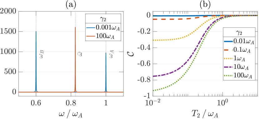
Figure 2: Strong damping regime and synchronization. (a) Plot of the finite eigenvalue of ${\bm{\chi}}_{2}^{\prime\prime}(\omega)$ as a function of frequency, showing that a dominant common mode appears at strong damping. (b) Synchronization, measured by the Pearson coefficient (10), as a function of temperature $T_{2}/\omega_{A}$. Different curves refer to various $\gamma_{2}$ damping strengths. Here and in the following figures, $\omega_{B}=0.6\omega_{A}$.

Mutual synchronization between the two QHOs arises when, regardless of their detuning, they start to oscillate coherently at a common frequency. In the present setup, therefore, synchronization can occur at strong damping $\gamma_{2}\gg\omega_{l}$. To quantify synchronization, we consider the dynamics of local observables and the corresponding Pearson coefficient [83]. Focusing on the position operator of the QHOs, this indicator reads

$${\cal C}=\frac{\langle\delta x_{A}\delta x_{B}\rangle}{\sqrt{\langle\delta x_{A}\delta x_{A}\rangle\langle\delta x_{B}\delta x_{B}\rangle}}~{},$$ (10)

where

$$\langle\delta x_{l}\delta x_{l^{\prime}}\rangle ={\rm Tr}[x_{l}(t)x_{l^{\prime}}(t)\tilde{\rho}]-{\rm Tr}[x_{l}(t)\tilde{\rho}]{\rm Tr}[x_{l^{\prime}}(t)\tilde{\rho}]$$

$$=\int_{-\infty}^{+\infty}\frac{{\rm d}\omega}{4\pi m}\coth(\frac{\omega}{2T_{2}}){\chi_{2}^{(l,l^{\prime})}}^{\prime\prime}(\omega)~{},$$ (11)

with $\tilde{\rho}=\exp\{-[\sum_{l=A,B}H_{l}+H_{2}+H_{{\rm int},2,l}]/T_{2}\}$. The Pearson coefficient takes values between $-1$ and $+1$, respectively denoting perfect temporal anti-synchronization and synchronization of the local observables. The value $0$, instead, denotes the absence of synchronization [83]. In Fig. 2(b) the behaviour of the Pearson coefficient for our setup with different values of the damping strength $\gamma_{2}$ is reported. This clearly shows that at sufficiently strong damping the two subsystems become synchronized and in anti-phase, reaching ${\cal C}\to-1$ at low temperature. At high temperature this feature is smeared out, with Pearson coefficient ${\cal C}\to 0$. In the opposite, weak damping regime instead ${\cal C}$ is always small, indicating no synchronization.

II.4 TUR violation for local power

In the following, we will investigate the local powers and associated TURs. We will focus on the regime of strong damping and emphasize the role of synchronization to find parameter regions where useful, nonvanishing subsystem power ($P_{l}<0$ and sizeable magnitude) can be obtained with high accuracy ($Q_{P_{l}}\ll 2$).

At the lowest perturbative order in the $\nu=1$ WM-bath interaction, the subsystem power contributions can be written as (see Appendix B for details)

$$P_{l}=P_{l}^{(0)}+\delta P_{l},$$ (12)

with

$$P_{l}^{(0)}=-\Omega\int_{-\infty}^{+\infty}\frac{{\rm d}\omega}{4\pi m}\mathcal{J}_{1}(\omega+\Omega)N(\omega,\Omega)$$

$$\quad\quad\quad\times\left[{\chi_{2}^{(l,l)}}^{\prime\prime}(\omega)+\cos(\phi){\chi_{2}^{(l,{\bar{l}})}}^{\prime\prime}(\omega)\right],$$ (13)

$$\delta P_{A/B}\!=\!\mp\Omega\sin(\phi)\int_{-\infty}^{+\infty}\!\!\!\frac{{\rm d}\omega}{4\pi m}\bigg{[}{\cal J}_{1}(\omega+\Omega){\chi_{2}^{(A,B)}}^{\prime}\!(\omega)$$

$$\!\!\times\!\coth\!\left(\!\frac{\omega\!+\!\Omega}{2T_{1}}\!\right)\!\!-\!m(\omega\!+\!\Omega)\gamma_{1}^{\prime\prime}\!(\omega\!+\!\Omega){\chi_{2}^{(A,B)}}^{\prime\prime}\!\!(\omega)\!\coth\!\left(\!\frac{\omega}{2T_{2}}\!\right)\!\!\bigg{]}\!,$$ (14)

where the last line involves the imaginary part of the damping kernel of Eq. (3) in Fourier space, $\gamma_{1}(\omega)=\gamma_{1}^{\prime}(\omega)+i\gamma_{1}^{\prime\prime}(\omega)$, and we have introduced the function $N(\omega,\Omega)=\coth(\frac{\omega+\Omega}{2T_{1}})-\coth(\frac{\omega}{2T_{2}})$. It is worth to stress that the total power is given by $P=P_{A}^{(0)}+P_{B}^{(0)}$,

$$P=-\Omega\int_{-\infty}^{+\infty}\!\frac{{\rm d}\omega}{4\pi m}\mathcal{J}_{1}(\omega+\Omega)N(\omega,\Omega)$$

$$\times\!\Big{[}{\chi_{2}^{(A,A)}}^{\prime\prime}\!(\omega)\!+\!{\chi_{2}^{(B,B)}}^{\prime\prime}\!(\omega)\!+\!2\cos(\phi){\chi_{2}^{(A,B)}}^{\prime\prime}\!(\omega)\Big{]}~{}.$$ (15)

For the sake of completeness, we also report the expression for the $\nu=1$ heat current [70]

$$J_{1}=\int_{-\infty}^{+\infty}\!\frac{{\rm d}\omega}{4\pi m}(\omega+\Omega)\mathcal{J}_{1}(\omega+\Omega)N(\omega,\Omega)$$

$$\times\!\Big{[}{\chi_{2}^{(A,A)}}^{\prime\prime}\!(\omega)\!+\!{\chi_{2}^{(B,B)}}^{\prime\prime}\!(\omega)\!+\!2\cos(\phi){\chi_{2}^{(A,B)}}^{\prime\prime}\!(\omega)\Big{]},$$ (16)

and $J_{2}=-P-J_{1}$. It is worth to underline that both $P$ and $J_{\nu}$ have an even dependence on $\phi$ and depend on the imaginary part of the response functions $\chi_{2}^{(l,l^{\prime})}$ only. Importantly, the subsystem power has a new term $\delta P_{l}$ that contains an odd contribution in the phase $\phi$. As we discuss in a moment, this will play a crucial role in determining the TUR violation for the subsystems $l=A,B$ since it represents an explicit TRS-breaking term. Finally, regarding the fluctuations associated to the subsystem power at the lowest perturbative order (see Appendix B) one gets

$$D_{P_{l}}= \Omega^{2}\int_{-\infty}^{+\infty}\frac{{\rm d}\omega}{4\pi m}\mathcal{J}_{1}(\omega+\Omega)N(\omega,\Omega)$$

$$\times\coth\left(\frac{\omega}{2T_{2}}-\frac{\omega+\Omega}{2T_{1}}\right){\chi_{2}^{(l,l)}}^{\prime\prime}(\omega).$$ (17)

Hereafter, we discuss in detail results for the $l=A$ channel and we exploit the $\phi$ phase degree of freedom, setting it to $\phi=\pi/2$ to maximize the TRS-breaking contribution. Note that analogous results can be obtained for $l=B$ letting $\phi=3\pi/2$. As already mentioned, we assume a strictly Ohmic spectral function for the $\nu=2$ reservoir, ${\cal J}_{2}(\omega)=m\gamma_{2}\omega$, while the $\nu=1$ reservoir has an Ohmic spectral density in the Drude-Lorentz form

$${\cal J}_{1}(\omega)=m\gamma_{1}\frac{\omega}{1+\frac{\omega^{2}}{\omega_{c}^{2}}}~{},$$ (18)

with a cut-off frequency $\omega_{c}$. Notice that in the strictly Ohmic regime, when $\omega_{c}$ is the highest energy scale, one recovers a memory-less (local in time) response. Finite cut-off values $\omega_{c}$, instead, would in general imply non-Markovian effects [64, 84]. It is worth to note that finite (and small) values of $\omega_{c}$ can be engineered in the context of quantum circuits [85, 84, 86, 87] and have been already inspected in other related dissipative systems [60, 61, 62, 88]. With the spectral density of Eq. (18) the imaginary part of the damping kernel $\gamma_{1}^{\prime\prime}(\omega)$ appearing in Eq. (14) becomes $\gamma_{1}^{\prime\prime}(\omega)={\cal J}_{1}(\omega)/(m\omega_{c})$.

Although the two subsystems $l=A,B$ have no direct coupling, correlations between the two are mediated by the interaction with the $\nu=2$ common reservoir, and we here consider the regime of full synchronization achieved at strong damping $\gamma_{2}\gg\omega_{l}$. Physically, this situation results in a very efficient exchange of power contributions between the two subsystems $P_{A}$ and $P_{B}$. This can be first illustrated in the case of isothermal reservoirs, $T_{1}=T_{2}=T$, where the two subsystems can act as a work-to-work converter [49], e.g., $P_{B}\geq 0$ is absorbed as input and $P_{A}\leq 0$ is extracted as output (with an associated efficiency $\eta=-P_{A}/P_{B}\leq 1$). The total power remains positive due to the second law of thermodynamics (indeed $\dot{S}=P/T\geq 0$).

By direct inspection of Eq. (17), in the isothermal regime the fluctuations associated to $l=A$ reduce to $D_{P_{A}}=\Omega\coth(\Omega/(2T))P_{A}^{(0)}$, regardless of the shape of ${\cal J}_{1}(\omega)$, and

$$Q_{P_{A}}=\frac{\Omega}{T}\coth\left(\frac{\Omega}{2T}\right)\frac{PP_{A}^{(0)}}{P_{A}^{2}}=Q_{P}\frac{1+P_{B}^{(0)}/P_{A}^{(0)}}{(1+\delta P_{A}/P^{(0)}_{A})^{2}},$$ (19)

where $Q_{P}=\Omega\coth(\Omega/(2T))/T$. Since $Q_{P}\geq 2$ (see Appendix C), violations of the TUR for $Q_{P_{A}}$, if any, must originate from the last fraction in the r.h.s. of the equation. In particular, one is interested in large values of the denominator, and hence one should look for $\delta P_{A}/P_{A}^{(0)}\gg 1$.

In the adiabatic regime ($\Omega\ll\omega_{l},T$) one has

$$P_{l}^{(0)}\to\Omega^{2}\alpha_{l}^{({\rm ad})},$$

$$\delta P_{l}\to\Omega\delta\alpha^{({\rm ad})}_{l}~{},$$ (20)

and hence $P\propto\Omega^{2}$ and $P_{l}\propto\Omega$ at leading order. Here, we have introduced auxiliary functions $\alpha_{l}^{({\rm ad})}$ and $\delta\alpha_{l}^{({\rm ad})}$ that do not depend on the external frequency $\Omega$ anymore (see Appendix D). This leads to the adiabatic expansion for the local TUR:

$$Q^{({\rm ad})}_{P_{A}}=2\Omega^{2}(\alpha_{A}^{({\rm ad})}+\alpha_{B}^{({\rm ad})})\frac{\alpha_{A}^{({\rm ad})}}{{\delta\alpha_{A}^{({\rm ad})}}^{2}}~{}.$$ (21)

From the above expression, one expects a violation of the local TUR ($Q_{P_{A}}\leq 2$) at sufficiently small $\Omega$, regardless of the precise shape of the spectral density ${\cal J}_{1}(\omega)$. This is indeed the case, as shown in Fig. 3(a-b).

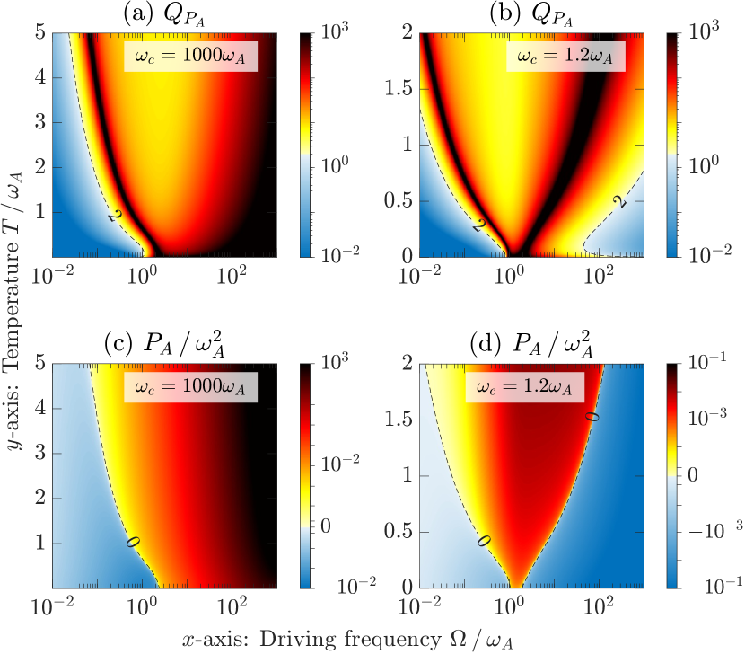
Figure 3: Quantifying fluctuations of $P_{A}$ via the trade-off quantity $Q_{P_{A}}$ in the isothermal regime. Density plots of $Q_{P_{A}}$ (a) and associated power $P_{A}$ (c) as a function of $\Omega/\omega_{A}$ and $T/\omega_{A}$ in the large cut-off regime $\omega_{c}=1000\omega_{A}$. Panels (b,d) report the same quantities as in panels (a,c), respectively, but for a small cut-off $\omega_{c}=1.2\omega_{A}$. All results have been obtained in the strong damping regime $\gamma_{2}=100\omega_{A}$; other parameters values are $\omega_{B}=0.6\omega_{A}$, $\gamma_{1}=0.01\omega_{A}$, and $\phi=\pi/2$. In panels (a,b) the dashed line denotes $Q_{P_{A}}=2$ separating regions where the TUR is violated (cool colors, $Q_{P_{A}}<2$) from regions where it is not (warm colors, $Q_{P_{A}}>2$). In panels (c,d) the dashed line refers to $P_{A}=0$ separating negative power contributions (power production, cool colors) from positive ones (power absorption, warm colors).

There, density plots of $Q_{P_{A}}$ in the $\Omega-T$ plane are reported for two different values of $\omega_{c}$, where a region with $Q_{P_{A}}<2$ is clearly visible in the left corner corresponding to $\Omega<\omega_{A}$. Looking at the corresponding power contribution $P_{A}$ (see panels c-d), one finds that $P_{A}<0$ in almost the same region, i.e., the system is acting as a work-to-work converter. This demonstrates that in the strong damping regime it is possible to obtain deviations from the TUR bound in the subsystem performance due to the breaking of TRS. However, violation of the TUR in this parameter regime is linked to small power magnitude, with $P_{A}\to\Omega{\delta\alpha}^{({\rm ad})}_{A}$ in the adiabatic limit. In passing we mention that for the $l=B$ channel at $\phi=\pi/2$ analogous TUR violation are observed but always with $P_{B}>0$ values, that is $l=B$ cannot be used as a useful resource for power production (see Supplementary Note 1). One may thus wonder if it is possible to achieve precise ($Q_{P_{A}}\ll 2$) but sizeable local power signals. To this end, the opposite, diabatic, regime ($\Omega\gg\omega_{l},\omega_{c}$) can be inspected. There, one obtains the following asymptotic expansions (see Appendix D)

$$P_{l}^{(0)}\to\Omega{\cal J}_{1}(\Omega)\alpha_{l}^{({\rm dia})},$$

$$\delta P_{l}\to\frac{\Omega^{2}}{\omega_{c}}{\cal J}_{1}(\Omega)\delta\alpha_{l}^{({\rm dia})}~{},$$ (22)

with the total power $P\propto\Omega{\cal J}_{1}(\Omega)$. Clearly, these expressions, and hence the behaviour of Eq. (19), depend on the shape of ${\cal J}_{1}(\omega)$ and on the value of the cut-off $\omega_{c}$. Indeed, one gets

$$Q_{P_{A}}^{({\rm dia})}=\frac{\Omega}{T}\frac{1+\alpha_{A}^{({\rm dia})}/\alpha_{B}^{({\rm dia})}}{\left[1+\tilde{{\cal C}}\frac{\Omega}{\omega_{c}}\right]^{2}},$$ (23)

where $\tilde{{\cal C}}=\delta\alpha_{A}^{({\rm dia})}/\alpha_{A}^{({\rm dia})}$. First of all, if one considers $\omega_{c}$ as the largest energy scale, thus with no memory effects, no TUR violations are expected (see the rightmost regions in the density plot of Fig. 3(a)). Intriguingly, the situation is different in the case of small cut-off $\omega_{c}$, i.e., when non-Markovian effects become important. Indeed, in the case of small $\omega_{c}$ and considering finite values of $\tilde{{\cal C}}$ one thus gets $Q_{P_{A}}^{({\rm dia})}\propto 1/\Omega$, which again shows the possibility to get $Q_{P_{A}}<2$. To corroborate this finding, in Fig. 3(b) the density plot of $Q_{P_{A}}$ in the $\Omega-T$ plane is reported for a representative small value $\omega_{c}=1.2\omega_{A}$. In this figure two regions where $Q_{P_{A}}<2$ are present: the first in the adiabatic regime, as discussed above, and a second new region in the diabatic regime $\Omega\gg\omega_{l},\omega_{c}$. The appearance of this new region is tightly bound to memory effects due to a finite cut-off $\omega_{c}$. More importantly, this latter regime is linked to finite power magnitude. This is indeed shown in Fig. 3(d), where a region with negative power contribution $P_{A}<0$ with sizeable magnitude is evident. Physically, in the diabatic regime $\Omega\gg\omega_{l},\omega_{c}$, the external frequency is much higher than the cut-off frequency of the reservoir that becomes effectively freezed, and the large amount of injected power from the $l=B$ channel is almost entirely transferred to the $l=A$ one, resulting in a very efficient work-to-work conversion with efficiency $\eta\sim 1$ (see Supplementary Note 2). We stress that in our model, in addition to TRS breaking, two are the key ingredients to achieve local TUR violation together with finite output power: memory effects and synchronization induced by strong damping $\gamma_{2}$. Interestingly, in the diabatic regime $\Omega\gg\omega_{l},\omega_{c}$, a quantity reminiscent of the Pearson coefficient of Eq. (10) naturally appears. Indeed, looking at the denominator in Eq. (23) one has $1+\tilde{{\cal C}}\Omega/\omega_{c}$. Inspecting the definition of $\tilde{{\cal C}}$ one finds that

$$\tilde{{\cal C}}=\frac{\langle\delta x_{A}\delta x_{B}\rangle}{\langle\delta x_{A}\delta x_{A}\rangle}={\cal C}\sqrt{\frac{\langle\delta x_{B}\delta x_{B}\rangle}{\langle\delta x_{A}\delta x_{A}\rangle}}~{},$$ (24)

and it is $|\tilde{{\cal C}}|<1$. The behaviour of this Pearson-like coefficient is qualitatively the same as the one reported in Fig. 2(b) for the Pearson coefficient ${\cal C}$. At low temperature $\tilde{{\cal C}}$ reaches values close to $-1$ in the strong damping regime when the two subsystems reach full synchronization being in anti-phase. This allows to get large values of the denominator in Eq. (23) that is a necessary condition to achieve TUR violation with sizeable power, clearly showing the importance of synchronization, established at strong damping. In Supplementary Note 3 for the sake of completeness we have reported the behaviour of the TUR and the subsystem power in the case of weak damping $\gamma_{2}$, where synchronization is lacking, showing that there the TUR for ${P_{A}}$ is not violated in the diabatic regime.

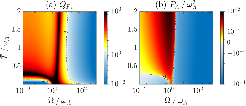
Figure 4: Quantifying fluctuations of $P_{A}$ via the trade-off quantity $Q_{P_{A}}$, in the presence of a temperature gradient in the strong damping regime $\gamma_{2}=100\omega_{A}$, with cut-off $\omega_{c}=1.2\omega_{A}$. Density plots of (a) $Q_{P_{A}}$ and (b) $P_{A}$ as a function of the driving frequency $\Omega/\omega_{A}$ and average temperature $\bar{T}/\omega_{A}$ at relative temperature gradient $\Delta T/\bar{T}=1.8$. Other parameters as in Fig. 3.

So far we have discussed results in the isothermal regime with $T_{1}=T_{2}=T$. Before closing, we now demonstrate the robustness of our results in the presence of a relative temperature gradient $\Delta T/\bar{T}$, with $\bar{T}=(T_{1}+T_{2})/2$ the average temperature and $\Delta T=T_{1}-T_{2}$ the temperature difference. Not only the presence of a region of TUR violation with sizeable power in the diabatic regime still holds with a finite temperature gradient, but also wider regions are obtained in the non-linear regime of temperature gradient. In Fig. 4(a,b) we show results for $Q_{P_{A}}$ and $P_{A}$, respectively, as a function of $\Omega$ and $\bar{T}$, at given $\Delta T/\bar{T}=1.8$. Notice that this last value implies a strong unbalance $T_{2}\ll T_{1}$ (strongly non-linear regime). At low driving frequencies, $\Omega<\omega_{A}$, the TUR for $P_{A}$ is violated for very low average temperature, $\bar{T}\lesssim 0.1\omega_{A}$. Instead, at higher driving frequencies the TUR is violated almost independently of the average temperatures considered, $0<\bar{T}<2\omega_{A}$. Comparing Fig. 4(b) and Fig. 3(b), we can see that the temperature gradient between the hot bath $\nu=1$ and the cold one $\nu=2$ can be exploited to greatly lower the driving frequency required to violate the TUR for $P_{A}$ (see also Supplementary Note 4).

III Discussion

We have shown that two otherwise independent quantum harmonic oscillators synchronize through coupling with a common thermal reservoir, at strong dissipation and low temperature. When the oscillators are also dynamically coupled to a second thermal reservoir, the synchronization regime can be exploited to achieve strong TURs violation for local powers. Such violation exploits breaking of TRS by dynamical couplings. It is remarkable that, in the diabatic regime and when the dynamically coupled bath is non-Markovian, both the power and the amount of TUR violation increase with the driving frequency.

Our results show the intimate connection between synchronization and thermodynamics of precision. From the standpoint of quantum technologies, synchronization mechanisms could be exploited to obtain finite and precise power in quantum circuits, where non-Markovian environments can be engineered [85, 84, 86, 87]. From a more general point of view, a thermodynamic perspective could also be useful in the broad field of classical synchronization.

Appendix A System-reservoir interactions

Here we provide some details on the microscopic model of the reservoirs and their couplings with the working medium of the quantum thermal machine. Following the Caldeira-Leggett approach [64], the $\nu$-th bath Hamiltonian reads

$$H_{{\nu}}=\sum_{k=1}^{+\infty}\left(\frac{P^{2}_{k,\nu}}{2m_{k,\nu}}+\frac{1}{2}m_{k,\nu}\omega^{2}_{k,\nu}X^{2}_{k,\nu}\right).$$ (25)

The bilinear form describing the WM-bath interactions is given by

$$H_{{\rm int},\nu}^{(t)}=\sum_{l=A,B}\sum_{k=1}^{+\infty}\bigg{[}-g_{\nu}^{(l)}(t)c_{k,\nu}x_{l}X_{k,\nu}$$

$$+\frac{(g_{\nu}^{(l)}(t)c_{k,\nu})^{2}}{2m_{k,\nu}\omega_{k,\nu}^{2}}x_{l}^{2}+\frac{g_{\nu}^{(l)}(t)g_{\nu}^{(\bar{l})}(t)c_{k,\nu}^{2}}{2m_{k,\nu}\omega_{k,\nu}^{2}}x_{l}x_{\bar{l}}\bigg{]}~{},$$ (26)

with $c_{k,\nu}$ describing the coupling strengths between the QHOs and the $k$-th mode of the $\nu$-th reservoir, modulated by the drives $g_{\nu}^{(l)}(t)$. In the above equation we used the convention according to which if $l=A$ then $\bar{l}=B$, and vice versa. Note that the superscript ^(t) reminds the time-dependent modulation $g_{1}^{(l)}(t)$. It is important to note that the interaction in Eq. (26) includes counter-term contributions having a twofold purpose: (i) to avoid renormalization of the characteristic frequencies $\omega_{A,B}$ of the QHOs and (ii) to cancel the direct coupling between the latter that would naturally arise [70].

At the initial time $t_{0}{\to-\infty}$ we assume that the reservoirs are in their thermal equilibrium at temperatures $T_{\nu}$ and that the total density matrix is in a factorized form $\rho(t_{0})=\rho_{A}(t_{0})\otimes\rho_{B}(t_{0})\otimes\rho_{1}(t_{0})\otimes\rho_{2}(t_{0})$, with $\rho_{l}(t_{0})$ the initial density matrix of the $l$-th QHO, and $\rho_{\nu}(t_{0})=\exp(-H_{\nu}/T_{\nu})/\Tr[\exp(-H_{\nu}/T_{\nu})]$ the thermal density matrix of the $\nu$-th reservoir.

Appendix B Derivation of power $P_{A}$ and associated fluctuations $D_{P_{A}}$

Here we provide details on the derivation of the subsystem average power $P_{l}$ and its fluctuations. We start from the definition in Eq. (5) and we first focus on the term present in the r.h.s.

$$\langle P_{l}(t)\rangle={\rm Tr}\bigg{[}\frac{\partial H_{{\rm int},1,l}^{(t)}(t)}{\partial t}\rho(t_{0})\bigg{]}~{},$$ (27)

where we have indicated with $\langle\cdot\rangle$ the quantum average. Denoting with $x_{l}^{(0)}(t)$ the unperturbed position operator, at the lowest perturbative order we obtain

$$\langle P_{l}(t)\rangle\!=\!\dot{g}_{1}^{(l)}(t)\Bigg{\{}\!i\!\sum_{l^{\prime}}\!\!\int_{t_{0}}^{t}\!\!\!\!{\rm d}s\,{\cal L}_{1}(s\!-\!t)g_{1}^{(l^{\prime})}\!(s)\big{\langle}\!\big{[}x_{l^{\prime}}^{(0)}\!(s),x^{(0)}_{l}\!(t)\big{]}\!\big{\rangle}$$

$$+\sum_{l^{\prime}}\int_{t_{0}}^{t}{\rm d}s\,\dot{{\Gamma}}_{1}(t\!-\!s)g_{1}^{(l^{\prime})}\!(s)\big{\langle}x^{(0)}_{l}\!(t)x^{(0)}_{l^{\prime}}\!(s)\big{\rangle}+g_{1}^{(l)}\!(t){\Gamma}_{1}(0)$$

$$\times\!\big{\langle}x_{l}^{(0)}\!(t)x_{l}^{(0)}\!(t)\big{\rangle}+g_{1}^{({\bar{l}})}\!(t){\Gamma}_{1}(0)\big{\langle}x_{l}^{(0)}(t)x_{{\bar{l}}}^{(0)}(t)\big{\rangle}\!\Bigg{\}}$$ (28)

where ${\Gamma}_{1}(t)$ is defined through Eq. (3) via $\gamma_{1}(t)=\frac{1}{m}\theta(t){\Gamma}_{1}(t)$. Here, we have introduced the symmetric and anti-symmetric contributions of the correlation function of Eq. (II.1) $\langle\xi_{\nu}(t)\xi_{\nu^{\prime}}(s)\rangle\equiv{\cal L}_{\nu}(t-s)\delta_{\nu,\nu^{\prime}}$, with ${\cal L}_{\nu}(t-s)={\cal L}_{\nu,{\rm s}}(t-s)+{\cal L}_{\nu,{\rm a}}(t-s)$ where

$${\cal L}_{\nu,{\rm s}}(t) =\int_{0}^{+\infty}\frac{\mathrm{d}\omega}{\pi}{\cal J}_{\nu}(\omega)\coth\left(\frac{\omega}{2T_{\nu}}\right)\cos(\omega t),$$ (29)

$${\cal L}_{\nu,{\rm a}}(t) =-i\int_{0}^{+\infty}\frac{\mathrm{d}\omega}{\pi}{\cal J}_{\nu}(\omega)\sin(\omega t).$$ (30)

Changing variable $\tau=t-s$ and introducing $C^{(l,l^{\prime})}(t-s)=C^{(l,l^{\prime})}(t,s)\equiv\big{\langle}x_{l}^{(0)}(t)x_{l^{\prime}}^{(0)}(s)\big{\rangle}$ we rewrite

$$\!\langle P_{l}(t)\rangle\!=\!i\sum_{l^{\prime}}\!\int_{0}^{+\infty}\!\!{\rm d}\tau\,{\cal L}_{1}(-\tau)G^{(l,l^{\prime})}(t,\tau)\Big{[}C^{(l^{\prime},l)}(-\tau)$$

$$\!-\!C^{(l,l^{\prime})}(\tau)\Big{]}+\!\sum_{l^{\prime}}\int_{0}^{+\infty}\!\!{\rm d}\tau\,\dot{\Gamma}_{1}(\tau)G^{(l,l^{\prime})}(t,\tau)C^{(l,l^{\prime})}(\tau)$$

$$\!+G^{(l,l)}(t,0)\Gamma_{1}(0)C^{(l,l)}(0)+G^{(l,{\bar{l}})}(t,0)\Gamma_{1}(0)C^{(l,{\bar{l}})}(0),$$ (31)

where ${\bar{l}}=B$ if $l=A$ (and viceversa), and we have introduced

$$G^{(l,l^{\prime})}(t,\tau)=\dot{g}_{1}^{(l)}(t)g_{1}^{(l^{\prime})}(t-\tau).$$ (32)

Recalling the identity

$$\dot{\Gamma}_{1}(t)=-2i{\cal L}_{1,{\rm a}}(t)~{},$$ (33)

introducing the average over the period and defining

$$G^{(l,l^{\prime})}(\tau)=\int_{0}^{{\cal T}}\frac{{\rm d}t}{{\cal T}}G^{(l,l^{\prime})}(t,\tau)$$ (34)

and the combination of correlators

$$C_{\pm}^{(l,l^{\prime})}(\tau)=C^{(l,l^{\prime})}(\tau)\pm C^{(l^{\prime},l)}(-\tau)$$ (35)

we get

$$P_{l}\!=\!-i\!\int_{0}^{+\infty}\!\!\!\!{\rm d}\tau\,{\cal L}_{1,{\rm s}}(\tau)\Big{[}G^{(l,l)}(\tau)C_{-}^{(l,l)}(\tau)$$

$$\!\!+\!G^{(l,\bar{l})}\!(\tau)C_{-}^{(l,\bar{l})}\!(\tau)\Big{]}\!\!-\!i\!\!\int_{0}^{+\infty}\!\!\!\!\!\!\!\!{\rm d}\tau\,{\cal L}_{1,{\rm a}}(\tau)\!\Big{[}G^{(l,l)}\!(\tau)C_{+}^{(l,l)}\!(\tau)$$

$$\!\!+\!G^{(l,\bar{l})}\!(\tau)C_{+}^{(l,\bar{l})}\!(\tau)\Big{]}\!\!+\!G^{(l,\bar{l})}\!(0)\Gamma_{1}(0)C^{(l,\bar{l})}\!(0).$$ (36)

Recalling Eqs. (29)–(30), we introduce the retarded Green function of the fluctuating force for the $\nu=1$ bath

$$\chi_{1}(t)\equiv i\theta(t)\langle\left[\xi_{1}(t),\xi_{1}(0)\right]\rangle=2i\theta(t){\cal L}_{1,{\rm a}}(t)$$ (37)

being ${\cal L}_{1,{\rm a}}(t)=\frac{1}{2}\left(\langle\xi_{1}(t)\xi_{1}(0)\rangle-\langle\xi_{1}(0)\xi_{1}(t)\rangle\right)$. The Fourier transform of the symmetric, ${\cal L}_{1,{\rm s}}(t)$, and anti-symmetric, ${\cal L}_{1,{\rm a}}(t)$, parts of ${\cal L}_{1}(t)$ read, respectively,

$${\cal L}_{1,{\rm s}}(\omega)={\cal J}_{1}(\omega)\coth\left(\frac{\omega}{2T_{1}}\right),\quad{\cal L}_{1,{\rm a}}(\omega)={\cal J}_{1}(\omega).$$ (38)

Using Eq. (37) and (38), it follows

$$\chi_{1}^{\prime\prime}(\omega)={\cal L}_{1,{\rm a}}(\omega)={\cal J}_{1}(\omega).$$ (39)

We introduce now a shifted response function

$$\zeta_{1}(\omega)=\chi_{1}(\omega)-\chi_{1}(\omega=0).$$ (40)

Using the relations introduced so far, it is possible to prove that real and imaginary part of the Fourier transform of the memory damping kernel $\gamma_{1}(t)$ in Eq. (3) are, respectively,

$$\gamma_{1}^{\prime}(\omega)=\frac{1}{m}\frac{\zeta_{1}^{\prime\prime}(\omega)}{\omega},\quad\gamma_{1}^{\prime\prime}(\omega)=-\frac{1}{m}\frac{\zeta_{1}^{\prime}(\omega)}{\omega},$$ (41)

which can be summarized into $\zeta_{1}(\omega)=im\omega\gamma_{1}(\omega)$. For a Ohmic spectral density with a Drude-Lorentz cut-off, ${\cal J}_{1}(\omega)=m\omega\gamma_{1}/(1+\omega^{2}/\omega_{c}^{2})$, as in the present setup, we have $\gamma_{1}^{\prime}(\omega)={\cal J}_{1}(\omega)/(m\omega)$ and $\gamma_{1}^{\prime\prime}(\omega)={\cal J}_{1}(\omega)/(m\omega_{c})$, from which

$$\zeta_{1}^{\prime}(\omega)=-\frac{\omega}{\omega_{c}}{\cal J}_{1}(\omega),\quad\zeta_{1}^{\prime\prime}(\omega)={\cal J}_{1}(\omega).$$ (42)

Now, considering the monochromatic drives of Eq. (2) and following similar steps as done in Ref. [70] we finally arrive at $P_{l}=P_{l}^{(0)}+\delta P_{l}$, where

$$P_{l}^{(0)}=-\Omega\int_{-\infty}^{+\infty}\frac{{\rm d}\omega}{4\pi m}\mathcal{J}_{1}(\omega+\Omega)N(\omega,\Omega)$$

$$\quad\quad\quad\times\left[{\chi_{2}^{(l,l)}}^{\prime\prime}(\omega)+\cos(\phi){\chi_{2}^{(l,\bar{l})}}^{\prime\prime}(\omega)\right],$$ (43)

$$\delta P_{A/B}=\mp\Omega\sin(\phi)\int_{-\infty}^{+\infty}\frac{{\rm d}\omega}{4\pi m}\left[\zeta_{1}^{\prime\prime}(\omega+\Omega){\chi_{2}^{(A,B)}}^{\prime}(\omega)\right.$$

$$\left.\times\coth\left(\frac{\omega+\Omega}{2T_{1}}\right)\!+\zeta_{1}^{\prime}(\omega+\Omega){\chi_{2}^{(A,B)}}^{\prime\prime}(\omega)\coth\left(\frac{\omega}{2T_{2}}\right)\right].$$ (44)

Notice that the total power is eventually given by $P=P_{A}^{(0)}+P_{B}^{(0)}$ and it is reported in the main text in Eq. (15). The expressions for the average heat currents can be derived analogously and are reported in Eq. (II.4). As a final remark we quote the expressions of the fluctuations for the separate power contributions obtained at the lowest perturbative order by following similar steps as outlined above:

$$D_{P_{l}}= \Omega^{2}\int_{-\infty}^{+\infty}\frac{{\rm d}\omega}{4\pi m}{\cal J}_{1}(\omega+\Omega)N(\omega,\Omega)$$

$$\times\coth(\frac{\omega}{2T_{2}}-\frac{\omega+\Omega}{2T_{1}}){\chi^{(l,l)}_{2}}^{\prime\prime}(\omega).$$ (45)

Finally, fluctuations associated to the total power at the lowest perturbative order are given by

$$\!\!D_{P}=\Omega^{2}\!\int_{-\infty}^{+\infty}\!\!\!\frac{{\rm d}\omega}{4\pi m}{\cal J}_{1}(\omega\!+\!\Omega)N(\omega,\Omega)\coth\!\left(\!\frac{\omega}{2T_{2}}\!-\!\frac{\omega\!+\!\Omega}{2T_{1}}\!\right)$$

$$\!\!\times\!\big{[}{\chi_{2}^{(A,A)}}^{\prime\prime}\!(\omega)\!+\!{\chi_{2}^{(B,B)}}^{\prime\prime}\!(\omega)\!+\!2\cos(\phi){\chi_{2}^{(A,B)}}^{\prime\prime}\!(\omega)\big{]}.$$ (46)

Notice that this quantity, unlike the average total power, is not just the sum of the two subsystem contributions, but it also includes mixed term proportional to $\cos(\phi)$.

Appendix C Proof of $Q_{P}\geq 2$

Here we will prove, by contradiction, that

$$Q_{P}=\dot{S}\frac{D_{P}}{P^{2}}\geq 2\,,$$ (47)

see Eq. (7). We start observing that Eq. (15) can be rewritten as

$$P=-\Omega\int_{-\infty}^{+\infty}\frac{\mathrm{d}\omega}{4\pi m}\mathcal{J}_{1}(\omega+\Omega)N(\omega,\Omega)\chi_{\mathrm{eff}}^{\prime\prime}(\omega)\,,$$ (48)

where we have introduced for compactness

$$\chi_{\mathrm{eff}}^{\prime\prime}(\omega)={\chi_{2}^{(A,A)}}^{\prime\prime}\!(\omega)\!+\!{\chi_{2}^{(B,B)}}^{\prime\prime}\!(\omega)\!+\!2\cos(\phi){\chi_{2}^{(A,B)}}^{\prime\prime}\,,$$ (49)

and we can similarly rewrite the expression of the total power fluctuations of Eq. (B). Finally, the entropy production rate $\dot{S}=-J_{1}/T_{1}+(P+J_{2})/T_{2}$ using Eqs. (15)-(II.4) reads

$$\dot{S}=2\!\int_{-\infty}^{+\infty}\!\!\!\frac{\mathrm{d}\omega}{4\pi m}\left(\!\frac{\omega}{2T_{2}}\!-\!\frac{\omega\!+\!\Omega}{2T_{1}}\!\right)\!\mathcal{J}_{1}(\omega\!+\!\Omega)N(\omega,\Omega)\chi_{\mathrm{eff}}^{\prime\prime}(\omega).$$ (50)

By plugging Eqs. (B), (48) and (50) into Eq. (47) and performing straightforward algebra, the following condition is found:

$$Q_{P}<2\implies I=\int_{-\infty}^{+\infty}\!\!\int_{-\infty}^{+\infty}\!\!\mathrm{d}\omega\mathrm{d}\omega^{\prime}\Phi_{\Omega}(\omega,\omega^{\prime})<0\,,$$ (51)

where

$$\Phi_{\Omega}(\omega,\omega^{\prime})=\chi_{\mathrm{eff}}^{\prime\prime}(\omega)\chi_{\mathrm{eff}}^{\prime\prime}(\omega^{\prime})\left[\lambda_{\omega}\coth(\lambda_{\omega^{\prime}})-1\right]$$

$$\times\mathcal{J}_{1}(\omega+\Omega)\mathcal{J}_{1}(\omega^{\prime}+\Omega)N(\omega,\Omega)N(\omega^{\prime},\Omega)\,,$$ (52)

and where $\lambda_{\omega}=\frac{\omega}{2T_{2}}-\frac{\omega+\Omega}{2T_{1}}$. We will now show that the condition of Eq. (51) can never be satisfied.

To begin with it is convenient to rewrite $I$ in a more symmetric form by noting that one can also write

$$I=\frac{1}{2}\int_{-\infty}^{+\infty}\int_{-\infty}^{+\infty}\mathrm{d}\omega\mathrm{d}\omega^{\prime}\left[\Phi_{\Omega}(\omega,\omega^{\prime})+\Phi_{\Omega}(\omega^{\prime},\omega)\right]\,.$$

Hence

$$I =\frac{1}{2}\int_{-\infty}^{+\infty}\int_{-\infty}^{+\infty}\mathrm{d}\omega\mathrm{d}\omega^{\prime}G(\omega,\omega^{\prime})\frac{N(\omega,\Omega)}{\lambda_{\omega}}\frac{N(\omega^{\prime},\Omega)}{\lambda_{\omega^{\prime}}}$$

$$\times\mathcal{J}_{1}(\omega+\Omega)\mathcal{J}_{1}(\omega^{\prime}+\Omega)\chi_{\mathrm{eff}}^{\prime\prime}(\omega)\chi_{\mathrm{eff}}^{\prime\prime}(\omega^{\prime})\,,$$ (53)

with

$$G(\omega,\omega^{\prime})\!=\!\lambda_{\omega}^{2}\!\left[\lambda_{\omega^{\prime}}\coth(\lambda_{\omega^{\prime}})\right]\!+\!\lambda_{\omega^{\prime}}^{2}\!\left[\lambda_{\omega}\coth(\lambda_{\omega})\right]\!-\!2\lambda_{\omega}\lambda_{\omega^{\prime}}.$$ (54)

Clearly, since $\lambda_{\omega}\coth(\lambda_{\omega})\geq 1$ one has $G(\omega,\omega^{\prime})\geq\left(\lambda_{\omega}-\lambda_{\omega^{\prime}}\right)^{2}\geq 0$ and therefore the sign of Eq. (C) is determined by the other factors in its integrand.

Now note that we can write

$$\frac{N(\omega,\Omega)}{\lambda_{\omega}}=\frac{\coth(\frac{\omega+\Omega}{2T_{1}})\coth(\frac{\omega}{2T_{2}})-1}{\left(\frac{\omega+\Omega}{2T_{1}}-\frac{\omega}{2T_{2}}\right)\coth(\frac{\omega+\Omega}{2T_{1}}-\frac{\omega}{2T_{2}})}\,,$$ (55)

where we have exploited the identity

$$\frac{\coth(x)-\coth(y)}{y-x}=\frac{\coth(x)\coth(y)-1}{(x-y)\coth(x-y)}\,.$$

The denominator of Eq. (55) is strictly positive, while the identity

$$\coth(x)\coth(y)-1=\frac{\cosh(x-y)}{\sinh(x)\sinh(y)}$$ (56)

implies $\mathrm{sgn}\{\coth(x)\coth(y)-1\}=\mathrm{sgn}\{xy\}$, the hyperbolic cosine (sine) being an even (odd) function, where $\mathrm{sgn}\{x\}$ is the sign of $x$. Therefore

$$\mathrm{sgn}\left\{\frac{N(\omega,\Omega)}{\lambda_{\omega}}\right\}=\mathrm{sgn}\{\omega(\omega+\Omega)\}\,.$$ (57)

One then concludes that the sign of the integrand in Eq. (C) is given by

$$\mathrm{sgn}\left\{(\omega+\Omega)\mathcal{J}_{1}(\omega+\Omega)\right\}\mathrm{sgn}\left\{(\omega^{\prime}+\Omega)\mathcal{J}_{1}(\omega^{\prime}+\Omega)\right\}$$

$$\times\mathrm{sgn}\left\{\omega\chi_{\mathrm{eff}}^{\prime\prime}(\omega)\right\}\mathrm{sgn}\left\{\omega^{\prime}\chi_{\mathrm{eff}}^{\prime\prime}(\omega^{\prime})\right\}\,.$$ (58)

Since $\mathcal{J}_{1}(\omega)$ is an odd function with $\mathcal{J}_{1}(\omega)\geq 0$ for $\omega\geq 0$, one immediately sees that $\mathrm{sgn}\left\{(\omega+\Omega)\mathcal{J}_{1}(\omega+\Omega)\right\}\geq 0$.

Finally, we have

$$\omega\chi_{\mathrm{eff}}^{\prime\prime}(\omega)=\gamma_{2}\omega^{2}\frac{\mathcal{N}(\omega)}{\left|\mathcal{D}(\omega)\right|^{2}}\,,$$ (59)

where

$$\mathcal{N}(\omega)= 2\omega^{4}+2\cos(\phi)(\omega^{2}-\omega_{A}^{2})(\omega^{2}-\omega_{B}^{2})$$

$$- 2\omega^{2}(\omega_{A}^{2}+\omega_{B}^{2})+\omega_{A}^{4}+\omega_{B}^{4}\,,$$ (60)

and where $\mathcal{D}(\omega)$ is given in Eq. (9). Here, $\mathcal{N}(\omega)$ is a quadratic form in $\omega^{2}$ with discriminant $-4(\omega_{A}^{2}-\omega_{B}^{2})^{2}\sin^{2}(\phi)\leq 0$, which proves that $\mathcal{N}(\omega)\geq 0$, whence we conclude that $\omega\chi_{\mathrm{eff}}^{\prime\prime}(\omega)\geq 0$. This finally shows that the integrand of Eq. (C) is non-negative and thus $I\geq 0$, contradicting the condition stated in Eq. (51). Thus, it is proven that $Q_{P}\geq 2$.

Appendix D Asymptotic expressions

Here we report the expressions of the various power contributions in the two opposite regimes of small and large external frequency $\Omega$. These expressions are evaluated at phase $\phi=\pi/2$.

In the adiabatic regime $\Omega\ll\omega_{l}$ the total power expansion reads

$$P\to\Omega^{2}\sum_{l=A,B}\alpha_{l}^{({\rm ad})},$$ (61)

with

$$\alpha^{({\rm ad})}_{l}\!\!=\!-\!\!\!\int_{-\infty}^{+\infty}\!\!\!\!\frac{{\rm d}\omega}{4\pi m}\!\bigg{[}\!\dot{{\cal J}_{1}}(\omega)N(\omega,0)-\frac{{\cal J}_{1}(\omega)}{2T_{1}\sinh^{2}\!\big{(}\!\frac{\omega}{2T_{1}}\!\big{)}}\!\bigg{]}\!{\chi_{2}^{(l,l)}}^{\prime\prime}\!\!(\omega)$$ (62)

where we used the notation $\dot{f}(\omega)={\rm d}f(\omega)/{\rm d}\omega$. The subsystem power contributions instead become

$$P_{l}\sim\delta P_{l}\to\Omega{\delta\alpha}^{({\rm ad})}_{l},$$ (63)

where

$$\delta\alpha_{A/B}^{({\rm ad})}= \mp\int_{-\infty}^{+\infty}\!\!\!\frac{{\rm d}\omega}{4\pi m}\bigg{[}{\cal J}_{1}(\omega){\chi_{2}^{(A,B)}}^{\prime}\!(\omega)\coth\!\left(\!\frac{\omega\!}{2T_{1}}\!\right)$$

$$-m\omega\gamma_{1}^{\prime\prime}(\omega){\chi_{2}^{(A,B)}}^{\prime\prime}\!\!(\omega)\coth\!\left(\!\frac{\omega}{2T_{2}}\!\right)\!\!\bigg{]}.$$ (64)

The associated fluctuations start quadratically as

$$D^{({\rm ad})}_{P_{l}} =\Omega^{2}\int_{-\infty}^{+\infty}\frac{{\rm d}\omega}{4\pi m}{\cal J}_{1}(\omega)N(\omega,0)$$

$$\times\coth\left(\frac{\omega(T_{1}-T_{2})}{2T_{1}T_{2}}\right){\chi_{2}^{(l,l)}}^{\prime\prime}(\omega)~{}.$$ (65)

In the opposite diabatic regime $\Omega\gg\omega_{l},\omega_{c}$, one gets

$$P\to\Omega{\cal J}_{1}(\Omega)\sum_{l=A,B}\alpha_{l}^{({\rm dia})},$$ (66)

where

$$\alpha_{l}^{({\rm dia})}=\int_{-\infty}^{+\infty}\frac{{\rm d}\omega}{4\pi m}\coth\left(\frac{\omega}{2T_{2}}\right){\chi_{2}^{(l,l)}}^{\prime\prime}(\omega)~{}.$$ (67)

We also have

$$\delta P_{l}\to\Omega{\cal J}_{1}(\Omega)\left[\delta\alpha_{l}^{({\rm dia})}\frac{\Omega}{\omega_{c}}+\delta\beta^{({\rm dia})}_{l}\right]~{},$$ (68)

with

$$\delta\alpha^{({\rm dia})}_{A/B}=\pm\int_{-\infty}^{+\infty}\frac{{\rm d}\omega}{4\pi m}\coth\left(\frac{\omega}{2T_{2}}\right){\chi_{2}^{(A,B)}}^{\prime\prime}(\omega)~{}$$

$$\delta\beta^{({\rm dia})}_{A/B}=\mp\coth\left(\frac{\Omega}{2T_{1}}\right)\int_{-\infty}^{+\infty}\frac{{\rm d}\omega}{4\pi m}{\chi_{2}^{(A,B)}}^{\prime}(\omega)~{}.$$ (69)

Notice that the last term $\delta\beta_{l}^{({\rm dia})}$ can be discarded when $\Omega\gg\omega_{c}$. Finally, the associated fluctuations in the diabatic regime read

$$D^{({\rm dia})}_{P_{l}}\!\!=\!\Omega^{2}{\cal J}_{1}(\Omega)\!\coth\!\!\left(\!\frac{\Omega}{2T_{1}}\!\right)\!\!\int_{-\infty}^{+\infty}\!\!\!\!\frac{{\rm d}\omega}{4\pi m}\!\coth\!\!\left(\!\frac{\omega}{2T_{2}}\!\right)\!{\chi_{2}^{(l,l)}}^{\prime\prime}\!\!(\omega).$$ (70)

Author contributions

L. R., M. C., F. C., and M. S. developed the model and performed the calculations. M.S. conceived and together with G. B. supervised the study. All authors discussed the results and contributed to writing and revising the manuscript.

Data availability

Data sets generated during the current study are available from the corresponding author on reasonable request.

Competing interests

The authors declare no competing interests.

- [1] Huygens, C. Letters to de Sluse, (letters; no. 1333 of 24 February 1665, no. 1335 of 26 February 1665, no. 1345 of 6 March 1665) (Societe Hollandaise Des Sciences, Martinus Nijho, 1895).
- [2] Pikovsky, A., Rosenblum, M., & Kurths, J. Synchronization: A Universal Concept in Nonlinear Sciences (Cambridge University Press, Cambridge, 2003).
- [3] Heinrich, G., Ludwig, M., Qian, J., Kubala, B., & Marquardt, F. Collective Dynamics in Optomechanical Arrays. Phys. Rev. Lett. 107, 043603 (2011).
- [4] Giorgi, G. L., Galve, F., Manzano, G., Colet, P., & Zambrini, R. Quantum correlations and mutual synchronization. Phys. Rev. A 85, 052101 (2012).
- [5] Giorgi, G. L., Plastina, F., Francica, G., & Zambrini, R. Spontaneous synchronization and quantum correlation dynamics of open spin systems. Phys. Rev. A 88, 042115 (2013).
- [6] Manzano, G., Galve, F., Giorgi, G. L., Hernández-García, E., & Zambrini, R. Synchronization, quantum correlations and entanglement in oscillator networks. Sci. Rep. 3, 1439 (2013).
- [7] Lee, T. E., & Sadeghpour, H. R. Quantum Synchronization of Quantum van der Pol Oscillators with Trapped Ions. Phys. Rev. Lett. 111, 234101 (2013).
- [8] Walter, S., Nunnenkamp, A., & Bruder, C. Quantum Synchronization of a Driven Self-Sustained Oscillator. Phys. Rev. Lett. 112, 094102 (2014).
- [9] Bastidas, V. M., Omelchenko, I., Zakharova, A., Schöll, E., & Brandes, T. Quantum signatures of chimera states. Phys. Rev. E 92, 062924 (2015).
- [10] Benedetti, C., Galve, F., Mandarino, A., Paris, M. G. A., & Zambrini, R. Minimal model for spontaneous quantum synchronization. Phys. Rev. A 94, 052118 (2016).
- [11] Du, L., Fan, C.-H., Zhang, H.-X., & We, J.-H. Synchronization enhancement of indirectly coupled oscillators via periodic modulation in an optomechanical system. Sci. Rep. 7, 15834 (2017).
- [12] Witthaut, B., Wimberger, S., Burioni, R., & Timme, M. Classical synchronization indicates persistent entanglement in isolated quantum systems. Nat. Commun. 8, 14829 (2017).
- [13] Amitai, E., Lörch, N., Nunnenkamp, A., Walter, S., & Bruder, C. Synchronization of an optomechanical system to an external drive. Phys. Rev. A 95, 053858 (2017).
- [14] Geng, H., Du, L., Liu, H. D., & Yi, X. X. Enhancement of quantum synchronization in optomechanical system by modulating the couplings. J. Phys. Commun. 2, 025032 (2018).
- [15] Roulet, A., & Bruder, C. Synchronizing the Smallest Possible System. Phys. Rev. Lett. 121, 053601 (2018).
- [16] Roulet, A., & Bruder, C. Quantum Synchronization and Entanglement Generation. Phys. Rev. Lett. 121, 063601 (2018).
- [17] Es’haqi-Sani, N., Manzano, G., Zambrini, R., & Fazio, R. Synchronization along quantum trajectories. Phys. Rev. Res. 2, 023101 (2020).
- [18] Jaseem, N., Hajdušek, M., Vedral, V., Fazio, R., Kwek, L.-C., & Vinjanampathy, S. Quantum synchronization in nanoscale heat engines. Phys. Rev. E 101, 020201(R) (2020).
- [19] Murtadho, T., Vinjanampathy, S., & Thingna, J. Cooperation and Competition in Synchronous Open Quantum Systems. Phys. Rev. Lett. 131, 030401 (2023).
- [20] Esposito, M., Harbola, U., & Mukamel, S. Nonequilibrium fluctuations, fluctuation theorems, and counting statistics in quantum systems. Rev. Mod. Phys. 81, 1665 (2009).
- [21] Arrachea, L., Energy dynamics, heat production and heat-work conversion with qubits: toward the development of quantum machines. Rep. Prog. Phys. 86, 036501 (2023).
- [22] Sapienza, F., Cerisola, F. & Roncaglia, A.J. Correlations as a resource in quantum thermodynamics. Nat. Commun. 10, 2492 (2019).
- [23] Horodecki, M., & Oppenheim, J. Fundamental limitations for quantum and nanoscale thermodynamics. Nat. Commun. 4, 2059 (2013).
- [24] Rodrigues, F.L.S., & Lutz, E. Nonequilibrium thermodynamics of quantum coherence beyond linear response. Commun. Phys. 7, 61 (2024).
- [25] Arrachea, L., Mucciolo, E. R., Chamon, C., & Capaz, R. B. Microscopic model of a phononic refrigerator. Phys. Rev. B 86, 125424 (2012).
- [26] López, R., Simon, P., & Lee, M. Heat and charge transport in interacting nanoconductors driven by time-modulated temperatures. SciPost Phys. 16, 094 (2024).
- [27] Bercioux, D., Egger, R., Hänggi, P., & Thorwart, M. Focus on nonequilibrium fluctuation relations: from classical to quantum. New J. Phys. 17, 020201 (2015).
- [28] De Chiara, G. & Imparato, A. Quantum fluctuation theorem for dissipative processes. Phys. Rev. Res. 4, 023230 (2022).
- [29] Saryal, S., Gerry, M., Khait, I., Segal, D., & Agarwalla, B. K. Universal Bounds on Fluctuations in Continuous Thermal Machines. Phys. Rev. Lett. 127, 190603 (2021).
- [30] Barato, A. C., & U. Seifert, Thermodynamic Uncertainty Relation for Biomolecular Processes. Phys. Rev. Lett. 114, 158101 (2015).
- [31] Horowitz, J. M., & Gingrich, T. R. Proof of the finite-time thermodynamic uncertainty relation for steady-state currents. Phys. Rev. E 96, 020103 (2017).
- [32] Shiraishi, N., Saito, K., & Tasaki, H. Universal Trade-Off Relation between Power and Efficiency for Heat Engines. Phys. Rev. Lett. 117, 190601 (2016).
- [33] Timpanaro, A. M., Guarnieri, G., Goold, J., & Landi, G. T. Thermodynamic Uncertainty Relations from Exchange Fluctuation Theorems. Phys. Rev. Lett. 123, 090604 (2019).
- [34] Pal, S., Saryal, S., Segal, D., Mahesh, T. S., & Agarwalla, B. K., Experimental study of the thermodynamic uncertainty relation. Phys. Rev. Res. 2, 022044(R) (2020).
- [35] Koyuk, T., & Seifert, U. Thermodynamic Uncertainty Relation for Time-Dependent Driving. Phys. Rev. Lett. 125, 260604 (2020).
- [36] Proesmans, K. Precision-dissipation trade-off for driven stochastic systems. Commun. Phys. 6, 226 (2023).
- [37] Landi, G. T., Kewming, M. J., Mitchison, M. T., & Potts, P. P. Current fluctuations in open quantum systems: Bridging the gap between quantum continuous measurements and full counting statistics. Preprint at https://arxiv.org/abs/2303.04270 (2023).
- [38] Loutchko, D., Sughiyama, Y. , & Kobayashi, T. J. The Geometry of Thermodynamic Uncertainty Relations in Chemical Reaction Networks. Preprint at https://arxiv.org/abs/2308.04806 (2023).
- [39] Tesser, L., & Splettstoesser, J. Out-of-Equilibrium Fluctuation-Dissipation Bounds. Preprint at https://arxiv.org/abs/2309.17422 (2023).
- [40] Kamijima, T., Ito, S., Dechant, A., & Sagawa, T. Thermodynamic uncertainty relations for steady-state thermodynamics. Phys. Rev. E 107, L052101 (2023).
- [41] Taddei, F., & Fazio, R. Thermodynamic uncertainty relations for systems with broken time reversal symmetry: the case of superconducting hybrid systems. Phys. Rev. B 108, 115422 (2023).
- [42] Brandner, K., Hanazato, T., & Saito, K. Thermodynamic Bounds on Precision in Ballistic Multiterminal Transport. Phys. Rev. Lett. 120, 090601 (2018).
- [43] Cangemi, L. M., Carrega, M., De Candia, A., Cataudella, V., De Filippis, G., Sassetti, M., & Benenti, G. Optimal energy conversion through antiadiabatic driving breaking time-reversal symmetry. Phys. Rev. Res. 3, 013237 (2021).
- [44] Ptaszyński, K. Coherence-enhanced constancy of a quantum thermoelectric generator. Phys. Rev. B 98, 085425 (2018).
- [45] Agarwalla, B. K., & Segal, D. Assessing the validity of the thermodynamic uncertainty relation in quantum systems. Phys. Rev. B 98, 155438 (2018).
- [46] Liu, J., & Segal, D. Thermodynamic uncertainty relation in quantum thermoelectric junctions. Phys. Rev. E 99, 062141 (2019).
- [47] Miller, H. J. D., Mohammady, M. H., Perarnau-Llobet, M., & Guarnieri, G. Thermodynamic Uncertainty Relation in Slowly Driven Quantum Heat Engines. Phys. Rev. Lett. 126, 210603 (2021).
- [48] Guarnieri, G., Landi, G. T., Clark, S. R., & Goold, J. Thermodynamics of precision in quantum nonequilibrium steady states. Phys. Rev. Res. 1, 033021 (2019).
- [49] Cangemi, L. M., Cataudella, V., Benenti, G., Sassetti, M., & De Filippis, G. Violation of TUR in a periodically driven work-to-work converter from weak to strong dissipation. Phys. Rev. B 102, 165418 (2020).
- [50] Rignon-Bret, A., Guarnieri, G., Goold, J., & Mitchison, M. T. Thermodynamics of precision in quantum nanomachines. Phys. Rev. E 103, 012133 (2021).
- [51] Kalaee, A. A. S., Wacker, A., & Potts, P. P. Violating the thermodynamic uncertainty relation in the three-level maser. Phys. Rev. E 104, L012103 (2021).
- [52] Tanogami, T., Vu, T. W., & Saito, K. Universal bounds on the performance of information-thermodynamic engine. Phys. Rev. Res. 5, 043280 (2023).
- [53] Gramajo, A. L. , Paladino, E., Pekola, J., & Fazio, R. Fluctuations and stability of a fast driven Otto cycle Phys. Rev. B 107, 195437 (2023).
- [54] Singh, V., Shaghaghi, V. Müstecaplıoğlu, Ö. E., and Rosa, D. Thermodynamic uncertainty relation in nondegenerate and degenerate maser heat engines. Phys. Rev. A 108, 032203 (2023).
- [55] López, R., Lim, J. S., & Kim, K. W. Optimal superconducting hybrid machine. Phys. Rev. Res. 5, 013038 (2023).
- [56] Mohanta, S., Saha, M., Venkatesh, B. P., & Agarwalla, B. K. Study of bounds on non-equilibrium fluctuations for asymmetrically driven quantum Otto engine. Phys. Rev. E 108, 014118 (2022).
- [57] Reiche, D., Hsiang, J.-T., & Hu, B.-L. Quantum Thermodynamic Uncertainty Relations, Generalized Current and Nonequilibrium Fluctuation-Dissipation Inequalities. Entropy 24, 1016 (2022).
- [58] Das, A., Mahunta, S., Agarwalla, B. K., & Mukherjee, V. Precision bound and optimal control in periodically modulated continuous quantum thermal machines Phys. Rev. E 108, 014137 (2023).
- [59] Acciai, M., Tesser, L., Eriksson, J., Sánchez, R., Whitney, R. S., and Splettstoesser, J. Constraints between entropy production and its fluctuations in nonthermal engines. Phys. Rev. B 109, 075405 (2024).
- [60] Frigerio, M., Hesabi, S., Afshar, D., & Paris, M. G. A. Exploiting Gaussian steering to probe non-Markovianity due to the interaction with a structured environment. Phys. Rev. A 104, 052203 (2021).
- [61] Wang, H., Thoss, M., Sorge, K. L., Gelabert, R., Jimenez, X., & Miller, W. H. Semiclassical description of quantum coherence effects and their quenching: a forward backward initial value representation study. J. Chem. Phys. 114, 2562 (2001).
- [62] Goychuk, I., & Hanggi, P. Quantum dynamics in strong fluctuating fields. Adv. Phys. 54, 525 (2005).
- [63] Caldeira, A. O., & Leggett, A. J. Quantum tunnelling in a dissipative system. Ann. Phys. 149, 374 (1983).
- [64] Weiss, U. Quantum Dissipative Systems - 5th Edition (World Scientific, Singapore, 2021).
- [65] Aurell, E. Characteristic functions of quantum heat with baths at different temperatures. Phys. Rev. E 97, 062117 (2018).
- [66] Leitch, H., Piccione, N., Bellomo, B., & De Chiara, G. Driven quantum harmonic oscillators: A working medium for thermal machines. AVS Quantum Sci. 4(1), 012001 (2022).
- [67] Carrega, M., Cangemi, L. M., De Filippis, G., Cataudella, V., Benenti, G., & Sassetti, M. Engineering Dynamical Couplings for Quantum Thermodynamic Tasks. PRX Quantum 3, 010323 (2022).
- [68] Cavaliere, F., Carrega, M., De Filippis, G., Cataudella, V., Benenti, G., & Sassetti, M. Dynamical heat engines with non-Markovian reservoirs. Phys. Rev. Res. 4, 033233 (2022).
- [69] Cavaliere, F., Razzoli, L., Carrega, M., Benenti, G., & Sassetti, M. Hybrid quantum thermal machines with dynamical couplings iScience 26, 106235 (2023).
- [70] Carrega, M., Razzoli, L., Erdman, P. A., Cavaliere, F., Benenti, G., & Sassetti, M. Dissipation-induced collective advantage of a quantum thermal machine. AVS Quantum Sci. 6, 025001 (2024).
- [71] Thorwart, M., Paladino, E., & Grifoni, M. Dynamics of the spin-boson model with a structured environment. Chem. Phys. 296, 333 (2004).
- [72] Paladino, E., Maugeri, A. G., Sassetti, M., Falci, G., & Weiss, U. Structured environments in solid state systems: Crossover from Gaussian to non-Gaussian behavior. Physica E 40, 198 (2007).
- [73] Iles-Smith, J., Lambert, N., & Nazir, A. Environmental dynamics, correlations, and the emergence of noncanonical equilibrium states in open quantum systems. Phys. Rev. A 90, 032114 (2014).
- [74] Strasberg, P., Schaller, G., Lambert, N., & Brandes, T. Nonequilibrium thermodynamics in the strong coupling and non-Markovian regime based on a reaction coordinate mapping. New J. Phys. 18, 073007 (2016).
- [75] Restrepo, S., Cerrillo, J., Strasberg, P., & Schaller, G. From quantum heat engines to laser cooling: Floquet theory beyond the Born-Markov approximation New J. Phys. 20, 053063 (2018).
- [76] Landi, G. T., & Paternostro, M. Irreversible entropy production: From classical to quantum. Rev. Mod. Phys. 93, 035008 (2021).
- [77] Esposito, M., Lindenberg, K., & Van den Broeck, C. Entropy production as correlation between system and reservoir. New J. Phys. 12, 013013 (2010).
- [78] Razzoli, L., Cavaliere, F., Carrega, M., Sassetti, M., & Benenti, G. Efficiency and thermodynamic uncertainty relations of a dynamical quantum heat engine. Eur. Phys. J. Spec. Top. (2023).
- [79] Paz, J. P., & Roncaglia, A. J. Dynamical phases for the evolution of the entanglement between two oscillators coupled to the same environment. Phys. Rev. A 79, 032102 (2009).
- [80] Galve, F., Giorgi, G. L., & Zambrini, R. Entanglement dynamics of nonidentical oscillators under decohering environments. Phys. Rev. A 81, 062117 (2010).
- [81] Correa, L. A., Valido, A. A., & Alonso, D. Asymptotic discord and entanglement of nonresonant harmonic oscillators under weak and strong dissipation. Phys. Rev. A 86, 012110 (2012).
- [82] Brenes, M., Min, B., Anto-Sztrikacs, N., Bar-Gill, N., & Segal, D. Bath-induced interactions and transient dynamics in open quantum systems at strong coupling: Effective Hamiltonian approach. Preprint at https://arxiv.org/abs/2403.03386 (2024).
- [83] Galve, F., Giorgi, G. L., & Zambrini, R. Quantum correlations and synchronization measures in Lectures on General Quantum Correlations and Their Applications (ed. Fanchini, F. F., Pinto, D. d. O. S., & Adesso, G.), pp. 393–420 (Springer, Berlin, 2017).
- [84] Cattaneo, M., & Paraoanu, G.-S. Engineering dissipation with resistive elements in circuit quantum electrodynamics. Adv. Quantum Technol. 4, 210054 (2021).
- [85] Gramich, V., Solinas, P., Mottonen, M., Pekola, J. P., & Ankerhold, J. Measurement scheme for the Lamb shift in a superconducting circuit with broadband environment. Phys. Rev. A 84, 052103 (2011).
- [86] Vaaranta, A., Cattaneo, M., and Lake, R. E. Dynamics of a dispersively coupled transmon qubit in the presence of a noise source embedded in the control line. Phys. Rev. A 106, 042605 (2022).
- [87] Kadijani, S. S., Schmidt, T. L., Esposito, M., & Freitas, N. Heat transport in overdamped quantum systems. Phys. Rev. B 102, 235422 (2020).
- [88] Tao, G. Electronically non adiabatic dynamics in singlet fission: a quasi-classical trajectory simulation. J. Phys. Chem. C 118, 17299 (2014).