Abstract

Discrete flavor symmetries provide a promising approach to understand the flavor sector of the standard model of particle physics. Top-down (TD) explanations from string theory reveal two different types of such flavor symmetries: traditional and modular flavor symmetries that combine to the eclectic flavor group. There have been many bottom-up (BU) constructions to fit experimental data within this scheme. We compare TD and BU constructions to identify the most promising groups and try to give a unified description. Although there is some progress in joining BU and TD approaches, we point out some gaps that have to be closed with future model building.

1 1 0 https://doi.org/ Flavor’s Delight Flavor’s Delight Hans Peter Nilles ¹ and Saúl Ramos-Sánchez ^2,* Hans Peter Nilles and Saúl Ramos-Sánchez Nilles, H.P.; Ramos-Sánchez, S. Correspondence: ramos@fisica.unam.mx

1 Introduction

The problem of flavor, the description of masses and mixing angles of quarks and leptons, remains one of the most important questions in elementary particle physics. A major approach to solve this problem is based on non-Abelian (discrete) flavor symmetries. In attempts to fit presently available data, many different symmetries and representations of flavor groups have been suggested and analysed. A comprehensive summary of these BU attempts can be found in the reviews Feruglio and Romanino (2021); Kobayashi and Tanimoto (2023); Chauhan et al. (2023); Ding and King (2023). In his book Frampton and Kim (2020) with Jihn E. Kim entitled “History of Particle Theory”, Paul Frampton (p.172) mentions his preferred flavor group $T^{\prime}$, the binary tetrahedral group. This choice is motivated through his early work on flavor symmetries: see ref. Frampton et al. (2008) and references therein.

Most attempts in the BU approach focus on the lepton sector to obtain solutions close to neutrino tribimaximal mixing Harrison et al. (2002). Prominent examples have been $A_{4}$, $S_{4}$, $\Delta(27)$, $\Delta(54)$, $\Sigma(81)$, $Q(24)$ among many others Ma (2008). While they lead to acceptable solutions in the lepton sector, applications to the quark sector have been less frequent and usually less successful. Still, as there are many viable models it is difficult to draw a definite conclusion about the correct choice.

It seems that we need additional ingredients to select models from a more theoretical point of view. Such TD considerations draw their motivation from string theory model building, in particular orbifold compactifications of the heterotic string Bailin and Love (1999); Nilles et al. (2009); Ramos-Sánchez (2009); Vaudrevange (2008); Nilles and Vaudrevange (2015); Ramos-Sánchez and Ratz (2024). Early work Kobayashi et al. (2007) on the $\mathbbm{Z}_{3}$ orbifold revealed the discrete flavor group $\Delta(54)$ with irreducible triplet representations to describe the three families of quarks and leptons. Even more earlier work, analyzing duality symmetries in string theory Lauer et al. (1989); Lerche et al. (1989); Chun et al. (1989); Lauer et al. (1991), provided an example of the discrete (modular) group $T^{\prime}$. From this point of view the predictions of the $\mathbbm{Z}_{3}$ orbifold lead to the discrete groups $\Delta(54)$ and $T^{\prime}$.

Fortunately, these groups allow many connections to models of the BU approach, were in fact $T^{\prime}$ and $\Delta(54)$ as well as their “little sisters” $A_{4}$ and $\Delta(27)$ have played a major role. In the following we want to analyze these specific constructions in detail. In section 2 we start with the tetrahedral group $T$ (isomorphic to the group $A_{4}$ of even permutations of 4 objects) that played a major role in the discussion of neutrino tribimaximal mixing. We continue with its double cover $T^{\prime}$ and potential applications to flavor physics. Section 3 introduces the motivation for the use of the group $\Delta(27)$ for leptonic mixing. It has 27 elements and is a discrete subgroup of $\mathrm{SU}(3)$. It is also a subgroup of $\Delta(54)$ that appeared in early discussions of flavor groups in string theory constructions Kobayashi et al. (2007). Section 4 is devoted to TD considerations of flavor symmetries from string theory model building. There, we shall also introduce the concept of discrete modular symmetries that were discovered from an analysis of dualities in string theory Lauer et al. (1989); Lerche et al. (1989); Chun et al. (1989); Lauer et al. (1991). The application of modular symmetries to flavor physics was pioneered in the BU approach by Feruglio Feruglio (2019) for the example of the discrete modular group $A_{4}$. We argue that the TD approach favors instead the modular flavor group $T^{\prime}$, the double cover of $A_{4}$. Section 5 introduces the concept of the eclectic flavor group Nilles et al. (2020a, b) that appears as a prediction in the string theory framework. It combines the traditional flavor symmetries (here $\Delta(54)$) with the discrete modular flavor symmetries (here $T^{\prime}$). In section 6 we shall try to make contact between the BU and TD approaches. Section 7 will give an outlook on strategies for further model building. The appendices will give technical details of the properties of $A_{4}$, $T^{\prime}$, $\Delta(27)$ and $\Delta(54)$.

2 The tetrahedral group and its double cover

The symmetry group $T$ of the tetrahedron is one of the smallest non-Abelian discrete groups and found early applications in particle physics Wyler (1979); Branco et al. (1980). It has 12 elements and is isomorphic to $A_{4}$ the group of even permutations of four elements. There are three singlets $(\boldsymbol{1},\boldsymbol{1}^{\prime},\boldsymbol{1}^{\prime\prime})$ and one irreducible triplet representation. Detailed properties of $T\cong A_{4}$ can be found in Appendix A.1. The presence of the triplet representation makes it attractive for flavor physics with three families of quarks and leptons. It became particularly relevant for the discussion of (nearly) tribimaximal mixing Ma and Rajasekaran (2001); Altarelli and Feruglio (2005) in the lepton sector. An explicit discussion of this situation can be found in the reviews Feruglio and Romanino (2021); Ma (2008). Tribimaximal mixing Harrison et al. (2002) is characterized (up to phases) through the PMNS structure

$$U_{\mathrm{PMNS}}~{}=~{}\begin{pmatrix}\sqrt{\tfrac{2}{3}}&\tfrac{1}{\sqrt{3}}&0\\ -\tfrac{1}{\sqrt{6}}&\tfrac{1}{\sqrt{3}}&-\tfrac{1}{\sqrt{2}}\\ -\tfrac{1}{\sqrt{6}}&\tfrac{1}{\sqrt{3}}&\tfrac{1}{\sqrt{2}}\end{pmatrix}$$

and includes a $\mathbbm{Z}_{2}$$\times$$\mathbbm{Z}_{2}$ symmetry acting (in the neutrino mass basis) as $U=\operatorname{\mathrm{diag}}(-1,-1,1)$ and $V=\operatorname{\mathrm{diag}}(-1,1,-1)$. This symmetry is a subgroup of $S_{4}$, the group of permutations of four elements. Tribimaximal mixing, however, is not exactly realized in nature as it would imply that the (reactor) angle $\theta_{13}$ vanishes. The $\mathbbm{Z}_{2}$ transformation $V$ thus cannot be an exact symmetry. This brings $A_{4}$ into the game, a subgroup of $S_{4}$ that does not contain $V$. It allows satisfactory fits for the lepton sector as reviewed in ref. Feruglio and Romanino (2021). These applications typically use the triplet representation for the left-handed lepton-$\mathrm{SU}(2)$-doublets $(\nu_{i},\ell_{i})$ and the representations $(\boldsymbol{1},\boldsymbol{1}^{\prime}$ and $\boldsymbol{1}^{\prime\prime})$ for the the $\mathrm{SU}(2)$ singlets of the standard model of particle physics (SM). Various “flavon” fields have to be considered for the spontaneous breakdown of $A_{4}$ and this is subject to explicit model building which we shall not discuss here in detail. In any case, $T\cong A_{4}$ is a very appealing discrete flavor symmetry for the description of the lepton sector.

A look at the quark sector reveals a completely different picture: there all mixing angles are small and a fit similar to the lepton sector does not seem to work. One particular property of the quark sector is the fact that the top-quark is much heavier than the other quarks. This seems to indicate a special role of the third family, somewhat sequestered from the other two families. It could therefore imply that for quarks the third-family is a singlet under the discrete flavor group. Such a situation can be well described in the framework of $T^{\prime}$, the double cover of $T\cong A_{4}$. This group has 24 elements with representations $\boldsymbol{1},\boldsymbol{1}^{\prime},\boldsymbol{1}^{\prime\prime},\boldsymbol{3}$ (as $A_{4}\cong T$) and in addition doublet representations $\boldsymbol{2},\boldsymbol{2}^{\prime},\boldsymbol{2}^{\prime\prime}$ (details of properties of $T^{\prime}$ can be found in Appendix A.2). This double-cover is similar to the double-cover $\mathrm{SU}(2)$ of $\mathrm{SO}(3)$ when describing angular momentum. In fact, $T$ is a subgroup of $\mathrm{SO}(3)$, and $T^{\prime}$ a subgroup of $\mathrm{SU}(2)$. This implies that the dynamics and constraints associated with $T$ can equally stem from the larger group $T^{\prime}$ (in analogy to the fact that one can also describe integer spin with $\mathrm{SU}(2)$), while the doublet representations of $T^{\prime}$ allow for more options Frampton and Kephart (1995, 2007).

This fact has been used in ref. Feruglio et al. (2007); Carr and Frampton (2007) to obtain a simultaneous description of both, the lepton- and the quark-sector in the framework of $T^{\prime}$ Frampton et al. (2008). The lepton sector remains the same as in the $A_{4}$ case while in the quark sector we do not use the irreducible triplet representation, but the representation $\boldsymbol{1}\oplus\boldsymbol{2}^{\prime}$, to single out the third family. This seems to be a nice explanation of the difference of the quark and lepton sectors within the flavor group $T^{\prime}$. As Paul Frampton says in his book with Jihn E. Kim Frampton and Kim (2020) (page 172) “Clearly, it is better simultaneously to fit both the quark- and lepton-mixing matrices. This is possible using, for example, the binary tetrahedral group $T^{\prime}$”. There are, of course, many other attempts based on larger groups and representations, but $T^{\prime}$ remains a very attractive option.

3 Towards larger groups: $\Delta(27)$ and $\Delta(54)$

Although small groups such as $A_{4}$ and $T^{\prime}$ already lead to satisfactory fits, there are a lot of new parameters and ambiguities in explicit model building and it is not evident whether this really gives the ultimate answer. In fact, there have been many more attempts with different groups and different representations as can be seen in the reviews ref. Feruglio and Romanino (2021); Kobayashi and Tanimoto (2023); Chauhan et al. (2023); Ding and King (2023). Another attractive small group is $\Delta(27)$. It has 27 elements, 9 one-dimensional representations as well as a triplet $\boldsymbol{3}$ and an anti-triplet $\bar{\boldsymbol{3}}$ representation. Technical details of the group are given in Appendix B.2. This is still a small group and it is attractive in particular because of the $\boldsymbol{3}$ and $\bar{\boldsymbol{3}}$ representations, which are well suited for flavor model building with three families of quarks and leptons. As shown in the appendix, it can be constructed as a semi-direct product of $\mathbbm{Z}_{3}$$\times$$\mathbbm{Z}_{3}$ and $\mathbbm{Z}_{3}$ and it is a subgroup of $\mathrm{SU}(3)$.

Early applications can be found in ref. Branco et al. (1984); de Medeiros Varzielas et al. (2007); Ma (2006, 2008); Luhn et al. (2007) which exploit the presence of the $\boldsymbol{3}$ and $\bar{\boldsymbol{3}}$ representations. For more recent work and a detailed list of references, we refer to ref. de Medeiros Varzielas et al. (2018); Cárcamo Hernández et al. (2024). As in the case of $A_{4}$, also $\Delta(27)$ is well suited to accommodate near tribimaximal mixing. Again (as for $A_{4}$), the $\mathbbm{Z}_{2}$$\times$$\mathbbm{Z}_{2}$ group of tribimaximal mixing is not a subgroup of $\Delta(27)$, but it appears approximately for specific alignments of vacuum expectation values of flavon fields that appear naturally within $\Delta(27)$.

$\Delta(27)$ is the “little sister” and subgroup of $\Delta(54)$. This group has 54 elements, two singlet, four doublet and two pairs of triplet and anti-triplet ($\boldsymbol{3}\oplus\bar{\boldsymbol{3}}$) representations. Properties of $\Delta(54)$ are collected in Appendix B.1. It is already quite a large group, somewhat unfamiliar to the BU flavor-community and found less applications than $\Delta(27)$. It became popular because of its appearance in string theory Kobayashi et al. (2007), which we shall discuss in section 4 in detail. Explicit BU model building with $\Delta(54)$ was pioneered in ref. Ishimori et al. (2009).

4 Top-Down considerations: A taste of flavor from string theory

In the BU approach there are many successful models based on various groups and representations Feruglio and Romanino (2021); Kobayashi and Tanimoto (2023); Chauhan et al. (2023); Ding and King (2023), too many to single out a “best” option. Such an answer might come from theoretical considerations and top-down model building. An attractive framework is given by string theory. Here we shall concentrate on orbifold compactifications of heterotic string theory that provide many realistic models with gauge group $\mathrm{SU}(3)$$\times$$\mathrm{SU}(2)$$\times$$\mathrm{U}(1)$ and three families of quarks and leptons Buchmüller et al. (2006); Lebedev et al. (2007a, b, 2008); Nilles et al. (2009); Nilles and Vaudrevange (2015); Olguín-Trejo et al. (2018); Perez-Martínez et al. (2021).

In these theories, discrete flavor symmetries arise as a result of the geometry of extra dimensions and the geography of fields localized in compact space. Strings are extended objects and this reflects itself in generalized aspects of geometry that include the winding modes of strings. A full classification of flavor symmetries of orbifold compactifications of the heterotic string is given by the outer automorphisms Baur et al. (2019a, b) of the Narain space group Narain (1986); Narain et al. (1987a, b); Groot Nibbelink and Vaudrevange (2017). Here we shall not be able to give a full derivation of this fact, but only provide a glimpse of the general TD formalism and illustrate the results in simple examples based on a $D=2$-dimensional torus and its orbifold.

In general, a string in $D$ dimensions has $D$ right-moving and $D$ left-moving degrees of freedom, encoded in $Y=(y_{\mathrm{R}},y_{\mathrm{L}})$. Compactifying the theory on a $D$-dimensional torus demands that the $2D$ degrees of freedom be subject to the toroidal boundary conditions

$$Y~{}=~{}\begin{pmatrix}y_{\mathrm{R}}\\ y_{\mathrm{L}}\end{pmatrix}~{}\sim~{}Y+E\,\hat{N}~{}=~{}\begin{pmatrix}y_{\mathrm{R}}\\ y_{\mathrm{L}}\end{pmatrix}+E\begin{pmatrix}n\\ m\end{pmatrix},$$

where the winding and the Kaluza-Klein (momentum) quantum numbers of the string, $n,m\in\mathbbm{Z}^{D}$, define a $2D$-dimensional Narain lattice. $E$ denotes the so-called Narain vielbein and contains the moduli $M_{i}$ of the torus. In the Narain formulation, we achieve a $D$-dimensional orbifold by imposing the identifications

$$Y\sim\Theta^{k}\,Y+E\,\hat{N},\quad\text{with the $\mathbbm{Z}_{K}$ orbifold twist}\quad\Theta=\begin{pmatrix}\theta_{\mathrm{R}}&0\\ 0&\theta_{\mathrm{L}}\end{pmatrix}\quad\text{satisfying}\quad\Theta^{K}=\mathbbm{1}_{2D}\,,$$

where $k=0,\ldots,K-1$ and the $\mathrm{SO}(D)$ elements $\theta_{\mathrm{L}},\theta_{\mathrm{R}}$ are set to be equal to obtain a symmetric orbifold. Excluding roto-translations, the Narain space group can then be generated by

$${\rm the\ twist}\ \ (\Theta,0)\ \ {\rm and\ shifts}\ \ (\mathbbm{1},E_{i})\ \ {\rm for}\ \ i=1,\ldots,2D\;.$$

It turns out that flavor symmetries correspond to the (rotational and translational) outer automorphisms of this Narain space group Baur et al. (2019a, b), which are transformations that map the group to itself but do not belong to the group.

Hence, it follows that the flavor symmetries of string theory come in two classes:

• Those symmetries that map momentum- to momentum- and winding- to winding-modes. These symmetries we call traditional flavor symmetries. They are the same type as those symmetries that would appear in a quantum field theory of point particles. In the Narain formulation, these can be understood as translational outer automorphisms of the Narain space group.

• Symmetries that exchange winding- and momentum-modes. They have their origin in duality transformations of string theory. We call them modular flavor symmetries as (for the torus discussed here) they are connected to the modular group $\mathrm{SL}(2,\mathbbm{Z})$. These arise from rotational outer automorphisms of the Narain space group.

4.1 Traditional flavor symmetries

Here we concentrate on the two-dimensional cases $\mathbbm{T}^{2}/\mathbbm{Z}_{K}$, $K=2,3,4,6$, that could be understood as the fundamental building blocks for the discussion of flavor symmetries. They have been discussed in detail in ref. Kobayashi et al. (2007). Various groups can be obtained, prominently $D_{8}$ or $\Delta(54)$. As an illustrative example we discuss here the case $\mathbbm{T}^{2}/\mathbbm{Z}_{3}$ with group $\Delta(54)$ because it has the nice property to provide irreducible triplet representations for three families of quarks and leptons Carballo-Pérez et al. (2016); Olguín-Trejo et al. (2018).

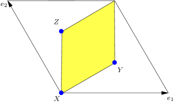
Figure 1: The $\mathbb{T}^{2}/\mathbbm{Z}_{3}$ orbifold (yellow shaded region) with three fixed points $X,Y,Z$. Twisted states are localized at theses fixed points. Figure taken from ref. Nilles et al. (2021).

The $\mathbbm{Z}_{3}$ orbifold $\mathbbm{T}^{2}/\mathbbm{Z}_{3}$ is shown in figure 1. Twisted fields are localized on the fixed points $X,Y,Z$ of the orbifold. This geometry leads to an $S_{3}$ symmetry from the interchange of the fixed points. String theory selection rules provide an additional $\mathbbm{Z}_{3}$$\times$$\mathbbm{Z}_{3}$ flavor symmetry as discussed in ref. Kobayashi et al. (2007). The full traditional flavor symmetry is $\Delta(54)$, the multiplicative closure of these groups. The twisted states on the fixed points $X,Y,Z$ transform as (irreducible) triplets under $\Delta(54)$ (details can be found in Appendix B.1). $\Delta(54)$ has two independent triplet representations $\boldsymbol{3}_{1}$ and $\boldsymbol{3}_{2}$. Both can be realized in string theory, depending on the presence or absence of twisted oscillator modes Nilles et al. (2020b). The untwisted states are in the trivial $\boldsymbol{1}$ representation in the absence and $\boldsymbol{1}^{\prime}$ in the presence of oscillator modes. A nontrivial vacuum expectation value of a field in the $\boldsymbol{1}^{\prime}$ representation will break $\Delta(54)$ to $\Delta(27)$. A discussion of the breakdown pattern of $\Delta(54)$ can be found in ref. Baur et al. (2022). Winding states transform as doublets under $\Delta(54)$. They are typically heavy and could play a prominent role in the discussion of $\mathcal{CP}$-violation in string theory as they provide a mechanism for baryogenesis through the decay of the heavy winding modes Nilles et al. (2018).

4.2 Modular flavor symmetries

They have their origin in duality transformations of string theory. One example is $T$-duality that exchanges winding and momentum modes. As a warm-up example consider a string on a circle of radius $R$.

The masses of momentum modes are governed by $1/R$, while winding states become heavier as $R$ grows. On the other hand, T-duality of string theory is defined by the transformations

$$\text{winding modes}~{}\longleftrightarrow~{}\text{momentum modes}\qquad\text{and}\qquad R~{}\longleftrightarrow~{}\alpha^{\prime}/R\;.$$

Hence, T-duality maps a theory to its T-dual, which coincides at the self-dual point $R^{2}=\alpha^{\prime}=1/M_{\rm string}^{2}$, where $1/\alpha^{\prime}$ is the string tension. For a generic value of the modulus $R$, T-duality exchanges light and heavy states, which suggests that T-duality could be relevant to flavor physics. Since string theory demands the compactifications of more than one extra dimension, T-duality generalizes to large groups of nontrivial transformations of the moduli of higher-dimensional tori. For instance, in $D=2$ the transformations on each of the (Kähler and complex structure) moduli build the modular group $\mathrm{SL}(2,\mathbbm{Z})^{2}$ of the $\mathbbm{T}^{2}$ torus. The group $\mathrm{SL}(2,\mathbbm{Z})$ is generated by two elements

$$\mathrm{S}\ \text{ and }\ \mathrm{T},\qquad\text{such that}\qquad\mathrm{S}^{4}~{}=~{}\mathbbm{1}\,,\qquad\mathrm{S}^{2}\mathrm{T}~{}=~{}\mathrm{T}\mathrm{S}^{2}\quad\text{and}\quad(\mathrm{S}\mathrm{T})^{3}~{}=~{}\mathbbm{1}\;.$$

For each modular group $\mathrm{SL}(2,\mathbbm{Z})$, there exists an associated modulus $M$ that transforms as

$$\mathrm{S}:\quad M~{}\mapsto~{}-{1\over M}\qquad\text{and}\qquad\mathrm{T}:\quad M~{}\mapsto~{}M+1\;.$$

Further transformations include mirror symmetry (that exchanges Kähler and complex structure moduli) as well as the $\mathcal{CP}$-like transformation

$$\mathrm{U}:\quad M~{}\mapsto~{}-\overline{M}\,,$$

where $\overline{M}$ denotes the complex conjugate of $M$. String dualities give important constraints on the action of the theory via the modular group $\mathrm{SL}(2,\mathbbm{Z})$ (or $\mathrm{GL}(2,\mathbbm{Z})$ when including $\mathrm{U}$). A general $\mathrm{SL}(2,\mathbbm{Z})$ transformation of the modulus is given by

$$M~{}\stackrel{{\scriptstyle\gamma}}{{\longmapsto}}~{}{{a\,M+b}\over{c\,M+d}},\qquad\gamma~{}=~{}\begin{pmatrix}a&b\\ c&d\end{pmatrix}~{}\in~{}\mathrm{SL}(2,\mathbbm{Z})$$

with $\det\gamma=1$ and $a,b,c,d\in\mathbbm{Z}$. The value of $M$ (originally in the upper complex half plane) is then restricted to the fundamental domain, as shown in (the dark shaded region of) figure 2. Matter fields $\phi$ turn out to transform as

$$\phi~{}\stackrel{{\scriptstyle\gamma}}{{\longmapsto}}~{}(c\,M+d)^{k}\rho(\gamma)\,\phi\qquad{\rm for}\qquad\gamma~{}\in~{}\mathrm{SL}(2,\mathbbm{Z})\;,$$

where $(c\,M+d)^{k}$ is known as automorphy factor, $k$ is a modular weight fixed by the compactification properties Ibáñez and Lüst (1992); Olguín-Trejo and Ramos-Sánchez (2017), and $\rho(\gamma)$ is a unitary representation of $\gamma$. Interestingly, $(\rho(\mathrm{T}))^{N}=\mathbbm{1}$ even though $\mathrm{T}^{N}\neq\mathbbm{1}$, such that $\rho(\gamma)$ generates a so-called finite modular group, as we shall shortly discuss. Among others, the modular weights $k$ of the fields are important ingredients for flavor model building.

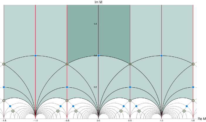
Figure 2: Fundamental domain of $\mathrm{SL}(2,\mathbbm{Z})$ (dark shaded) and of its subgroup $\Gamma(3)\cong\mathrm{SL}(2,3\mathbbm{Z})$ (light shaded). Figure taken from ref. Nilles et al. (2021)

.

As in the one-dimensional case, duality maps one theory to its dual and there remains the question whether such transformations are relevant for the low-energy effective action of the massless fields. This has been discussed explicitly with the help of worldsheet conformal field theory methods Lauer et al. (1989); Lerche et al. (1989); Chun et al. (1989); Lauer et al. (1991). It leads to field-dependent Yukawa couplings that transform as modular forms $Y^{(n_{Y})}(M)$ of a weights $n_{Y}>0$

$$Y^{(n_{Y})}(M)~{}\stackrel{{\scriptstyle\gamma}}{{\longmapsto}}~{}(c\,M+d)^{n_{Y}}\rho_{Y}(\gamma)\,Y^{(n_{Y})}(M)\quad\text{for}\quad\gamma~{}\in~{}\mathrm{SL}(2,\mathbbm{Z})\;,$$

where, as for matter fields, $\rho_{Y}(\gamma)$ is also a unitary representation of $\gamma$ in a finite modular group. The description in terms of supergravity actions has been given in ref. Ferrara et al. (1989). From the transformation properties of matter fields and Yukawa couplings, it becomes clear that the action is subject to both invariance under the finite modular group and conditions on the modular weights, which are strongly restricted in the TD approach.

Let us illustrate the relevance to flavor physics in the case of the $\mathbbm{Z}_{3}$ orbifold. We start with a two-torus and its two moduli: Kähler modulus $M$ and complex structure modulus $U$. On the orbifold the $U$-modulus is frozen, such that the lengths of the lattice vectors $e_{1}$ and $e_{2}$ are equal with an angle of 120 degrees (see figure 1). This also gives restrictions on the modular transformations of the matter fields. The coefficients $a,b,c,d\in\mathbbm{Z}$ of the modular transformation are defined only modulo 3; hence, instead of the full modular group $\mathrm{SL}(2,\mathbbm{Z})$, we have to deal with its so-called principal congruence subgroup, $\Gamma(3)\cong\mathrm{SL}(2,3\mathbbm{Z})$. Clearly, $\Gamma(3)$ has still infinitely many elements, but it is a normal subgroup of finite index in $\mathrm{SL}(2,\mathbbm{Z})$. Hence, a finite discrete modular group can be obtained by the quotient $\mathrm{SL}(2,\mathbbm{Z})/\Gamma(3)=\Gamma_{3}^{\prime}$. An explicit discussion is given in ref. de Adelhart Toorop et al. (2012). $\Gamma_{3}^{\prime}$ is isomorphic to $T^{\prime}$, the binary tetrahedral group. It is the double cover of $\Gamma_{3}\cong A_{4}$, which one would obtain starting with $\mathrm{PSL}(2,\mathbbm{Z})$ instead of $\mathrm{SL}(2,\mathbbm{Z})$. In the first application of discrete modular flavor symmetry Feruglio Feruglio (2019) used the group $\Gamma_{3}\cong A_{4}$ with its representations $\boldsymbol{1},\boldsymbol{1}^{\prime},\boldsymbol{1}^{\prime\prime}$ and $\boldsymbol{3}$ to explain tribimaximal mixing in the standard way. Complications with flavon fields and many additional parameters could be avoided as the modular flavor symmetry is nonlinearly realized. This might lead to problems with the control of additional free parameters in the Kähler potential that has been taken into account Chen et al. (2020). The modular flavor approach was picked up quickly Kobayashi et al. (2018); Penedo and Petcov (2019); Ding et al. (2019); Liu and Ding (2019); Liu et al. (2020); Liu and Ding (2022); Kobayashi and Tanimoto (2023); Ding and King (2023); Arriaga-Osante et al. (2023) and led to many different BU constructions with various groups, representations of modular weights.

Unfortunately, the TD approach is much more restrictive and allows less freedom in model building. In our example we obtain $T^{\prime}$ and not $A_{4}$ (the double cover is necessary to obtain chiral fermions in the string construction). Moreover, the twisted states do not transform as irreducible triplets of $T^{\prime}$ but as $\boldsymbol{1}\oplus\boldsymbol{2}^{\prime}$ and the modular weights of the fields are correlated with the $T^{\prime}$ representation (thus cannot be chosen freely as done in the BU framework). Some details of $T^{\prime}$ modular forms are given in Appendix C.

5 Eclectic flavor groups

So far we have seen that string theory predicts the presence of both, the traditional flavor group ($\Delta(54)$ in our example) and the modular flavor group ($T^{\prime}$). You cannot have one of them without the other. This should be taken into account in flavor model building. The eclectic flavor group Nilles et al. (2020a) is the multiplicative closure of $\Delta(54)$ and $T^{\prime}$, here $\Omega(1)=[648,533]$. Observe that this group has only 648 elements for the product of groups with 54 and 24 elements, respectively. There is one $\mathbbm{Z}_{2}$-like element contained in both $\Delta(54)$ and $T^{\prime}$. Incidentally, this is the same element that enhances $\Delta(27)$ to $\Delta(54)$. Thus $\Delta(27)$ and $\Delta(54)$, together with $T^{\prime}$, would lead to the same eclectic group Nilles et al. (2020a).

The eclectic flavor group is nonlinearly realized. Part of it appears “spontaneously” broken through the vacuum expectation value of the modulus $M$. The modulus is confined to the fundamental domain of $\Gamma(3)=\mathrm{SL}(2,3\mathbbm{Z})$ as displayed in figure 2. This area is reduced by a factor two if we include the natural candidate for a $\mathcal{CP}$-symmetry that transforms $M$ to $-\overline{M}$. The $\mathcal{CP}$-symmetry extends $\mathrm{SL}(2,\mathbbm{Z})$ to $\mathrm{GL}(2,\mathbbm{Z})$, $T^{\prime}$ to $\mathrm{GL}(2,3)$ (a group with 48 elements) and the eclectic group $\Omega(1)$ to a group with 1296 elements. The fundamental domain includes fixed points and fixed lines with respect to the modular transformations $\mathrm{S}$ and $\mathrm{T}$ as well as the $\mathcal{CP}$-transformation $\mathrm{U}:M\to-\overline{M}$ as shown in figure 3.

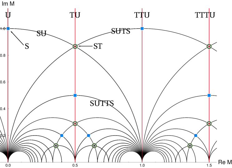
Figure 3: Unbroken modular symmetries at special curves in moduli space, including the $\mathcal{CP}$-like generator $\mathrm{U}$, which maps $M\mapsto-\overline{M}$. Figure adapted from ref. Baur et al. (2019b).

For generic points in moduli space the traditional flavor symmetry $\Delta(54)$ is linearly realized. At the fixed points and lines this symmetry is enhanced to larger groups as illustrated in figure 4.

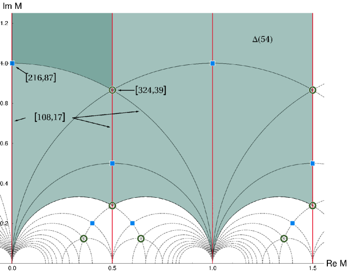
Figure 4: Local flavor unification at special points and curves in moduli space. The traditional flavor symmetry $\Delta(54)$, valid at generic points, is enhanced to two (different) groups with GAP Id [108,17] at the vertical lines and semi-circles, including $\mathcal{CP}$-like transformations. At the intersections of curves, the flavor symmetry is further enhanced to [216,87] and [324,39], also with $\mathcal{CP}$-like transformations. Figure adapted from ref. Baur et al. (2019a).

We see that here the largest linearly realized group has 324 elements with GAP Id [324,39]. (We use the group notation of the classification of GAP GAP .) Thus only part of the full eclectic flavor group with 1296 elements (including $\mathcal{CP}$) can be linearly realized. The enhancement of the traditional flavor symmetry at fixed loci (here points and lines) in the fundamental domain exhibits the phenomenon called “Local Flavor Unification” Baur et al. (2019a, b). The flavor symmetry is non-universal in moduli space and the spontaneous breakdown of modular flavor symmetry can be understood as a motion in moduli space. This has important consequences for flavor model building. At the loci of enhanced symmetry some of the masses and mixing angles of quark- and lepton-sector might vanish. The explanation of small parameters and hierarchies in flavor physics can thus find an explanation if the modulus is located close to the fixed points or lines Feruglio et al. (2021); Baur et al. (2022); Novichkov et al. (2022); Baur et al. (2022); Feruglio (2023); Hoshiya et al. (2022); Petcov and Tanimoto (2023); Abe et al. (2023); de Medeiros Varzielas et al. (2023); Ding et al. (2024). The mechanism of moduli stabilization in string theory could therefore provide the ingredients to understand the mysteries of flavor Kobayashi et al. (2019); Novichkov et al. (2022); Knapp-Pérez et al. (2023); Kobayashi et al. (2023).

6 Top-down does not yet meet bottom-up

There have been many BU constructions, but only a few that took into account TD considerations Chen et al. (2022); Ding et al. (2023); Li and Ding (2024). From the presently available TD models, the groups $\Delta(54)$ for traditional and $T^{\prime}$ for modular flavor symmetry seem to be the favourite choices. In fact, there is only one explicit model that incorporates the SM with gauge group $\mathrm{SU}(3)$$\times$$\mathrm{SU}(2)$$\times$$\mathrm{U}(1)$ and three families of quarks and leptons Baur et al. (2022). We certainly need more work in the TD approach. Therefore, any conclusions about the connection between the two approaches is necessarily preliminary. Still, it is reassuring to see that the same groups $\Delta(54)$ and $T^{\prime}$ and their “little sisters” $\Delta(27)$ and $A_{4}$ appear prominently in BU constructions. One could therefore try to make contact between the two approaches within this class of models.

Before we do that, we would like to stress some important properties of the TD approach that seem to be of more general validity and thus should have an influence on BU model building. The first of this is the prediction of string theory for the simultaneous presence of both, traditional and modular flavor symmetry that combine to the eclectic flavor group. It is this eclectic group which is relevant, not one of the others in isolation. Up to now, many BU constructions only consider one of them. Therefore, a direct contact between the two approaches is very difficult at this point.

The TD approach is very restrictive. Apart from the the limited type of groups that appear in the TD constructions, there are also severe restrictions on the choice of representations. Not everything is possible. In the case of modular symmetry $T^{\prime}$, for example, the irreducible triplet representation does not appear in the spectrum, while many BU constructions exactly concentrate on this representation. Therefore, the TD approach cannot make contact with models based on modular $A_{4}$ flavor symmetry where these triplets are generally used. For $T^{\prime}$ we have the twisted fields in the $\boldsymbol{1}\oplus\boldsymbol{2}^{\prime}$ representation. It seems to be more likely that irreducible triplet representations are found within the traditional flavor group, as seen in the example with $\Delta(54)$.

A second severe restriction concerns the choice of modular weights. In the TD approach we have essentially no choice. Once we know the representations of the eclectic group, the modular weights are fixed. This is an important restriction as in the BU approach the choice of modular weights is an important ingredient of model building. With a careful choice of modular weights one can create additional “shaping symmetries” which are important for the success of the fit to the data. This is not possible in the TD approach. There the role of such symmetries could, however, be found in the traditional flavor symmetry.

As a result of these facts, there is presently still a crucial difference between the BU and TD approaches and a direct comparison is not possible at this point. We are still at the very early stage of such investigations.

7 Outlook

Much more work in both approaches is needed to clarify the situation. In the BU approach it would be desirable to consider models that fulfill the restrictions coming from TD. Traditional flavor symmetries and the eclectic framework should be taken into account. A toolkit for such a construction can be found in the consideration of a modular group that fits into the outer automorphism of the traditional flavor group, as explained in ref. Nilles et al. (2020a). A recent application of this connection for the traditional flavor group $\Delta(27)$ has been discussed in ref. Ding et al. (2023); Li and Ding (2024). Moreover, BU constructions should avoid the excessive use of modular weights in model building. A strict correlation between the representations and their modular weights might be the right way to proceed. Useful shaping symmetries might be found within the traditional flavor symmetry instead.

The TD approach needs serious attempts for the construction of more explicit models. In particular, it would be useful to increase the number of explicit string constructions that ressemble the SM with gauge group $\mathrm{SU}(3)$$\times$$\mathrm{SU}(2)$$\times$$\mathrm{U}(1)$ and three families of quarks and leptons. This is important, as in generic string theory we might find huge classes of duality symmetries that might not survive in models with the properties of the SM. Of course, the size and nature of these large symmetry groups have to be explored. Modular invariance and its group $\mathrm{SL}(2,\mathbbm{Z})$ are closely related to torus compactifications, that can be realized in orbifold compactifications and more generally in Calabi-Yau compactifications with elliptic fibrations. This can be described by the basic building blocks $\mathbbm{T}^{2}/\mathbbm{Z}_{K}$ with $K=2,3,4,6$, which have been studied so far Nilles et al. (2021). Explicit string model building shows that such situations are possible, but require particular constellations for the Wilson lines needed for realistic model building. Such Wilson lines and other background fields might otherwise break modular symmetries in various ways Bailin et al. (1994); Lopes Cardoso et al. (1994); Love et al. (1994). In some orbifolds, only a subgroup of $\mathrm{SL}(2,\mathbbm{Z})$ is unbroken even without background fields Bailin et al. (1995), which opens up the possibility of finite modular flavor symmetries beyond $\Gamma^{\prime}_{K}$  Liu and Ding (2022); Ding et al. (2023); Arriaga-Osante et al. (2023). Yet a more general discussion has to go beyond $\mathrm{SL}(2,\mathbbm{Z})$. A first step in the direction is the consideration of the Siegel modular group Baur et al. (2020); Nilles et al. (2021); Ding et al. (2024) or higher dimensional constructions de Medeiros Varzielas et al. (2020); Nilles et al. (2020, 2021); Kikuchi et al. (2024). Many exciting developments seem to be in front of us.

The work by SR-S was partly funded by UNAM-PAPIIT grant IN113223 and Marcos Moshinsky Foundation.

No new data were created or analyzed in this study. Data sharing is not applicable to this article.

Appendix A The group $A_{4}$ and its double cover $T^{\prime}$

A.1 $A_{4}$

$A_{4}\cong(\mathbbm{Z}_{2}\times\mathbbm{Z}_{2})\rtimes\mathbbm{Z}_{3}$ (GAP Id [12,3]) is the alternating group of four elements and can also be understood as the rotational symmetry group of a regular tetrahedron. It contains 12 elements. $A_{4}$ has the irreducible representations $\boldsymbol{r}\in\{\boldsymbol{1},\boldsymbol{1}^{\prime},\boldsymbol{1}^{\prime\prime},\boldsymbol{3}\}$. With $\omega:=\mathrm{e}^{\nicefrac{{2\pi\mathrm{i}}}{{3}}}$, its character table reads

class	$1C_{1}$	$3C_{2}$	$4C_{3}$	$4C_{3}^{\prime}$
representative	$\mathbbm{1}$	$\mathrm{S}$	$\mathrm{T}$	$\mathrm{T}^{2}$
$\boldsymbol{1}$	$1$	$1$	$1$	$1$
$\boldsymbol{1}^{\prime}$	$1$	$1$	$\omega$	$\omega^{2}$
$\boldsymbol{1}^{\prime\prime}$	$1$	$1$	$\omega^{2}$	$\omega$
$\boldsymbol{3}$	$3$	$-1$	$0$	$0$

in terms of the generators $\mathrm{S}$ and $\mathrm{T}$. They satisfy $\mathrm{S}^{2}=\mathrm{T}^{3}=(\mathrm{ST})^{3}=\mathbbm{1}$ and their representations $\rho_{\boldsymbol{r}}$ can be expressed by

$\boldsymbol{r}$	$\boldsymbol{1}$	$\boldsymbol{1}^{\prime}$	$\boldsymbol{1}^{\prime\prime}$	$\boldsymbol{3}$
$\rho_{\boldsymbol{r}}(\mathrm{S})$	$1$	$1$	$1$	$\frac{1}{3}\begin{pmatrix}-1&2&-2\\ 2&-1&-2\\ -2&-2&-1\end{pmatrix}$
$\rho_{\boldsymbol{r}}(\mathrm{T})$	$1$	$\omega$	$\omega^{2}$	$\operatorname{\mathrm{diag}}(1,\omega,\omega^{2})$

The $A_{4}$ product rules are

$$\boldsymbol{1}^{a}\otimes\boldsymbol{1}^{b} =\boldsymbol{1}^{c}\ \ \text{with}\ \ c=a+b\!\!\!\mod 3,\ \ \boldsymbol{1}^{a}\otimes\boldsymbol{3}=\boldsymbol{3},\ \ \boldsymbol{3}\otimes\boldsymbol{3}=\boldsymbol{1}\oplus\boldsymbol{1}^{\prime}\oplus\boldsymbol{1}^{\prime\prime}\oplus\boldsymbol{3}\oplus\boldsymbol{3},$$

where $a,b,c=0,1,2$ correspond to the number of primes.

A.2 $T^{\prime}$

$T^{\prime}$ (GAP Id [24,3]) is the double cover of $A_{4}$ known also as binary tetrahedral group. Its irreducible representations are $\boldsymbol{r}\in\{\boldsymbol{1},\boldsymbol{1}^{\prime},\boldsymbol{1}^{\prime\prime},\boldsymbol{2},\boldsymbol{2}^{\prime},\boldsymbol{2}^{\prime\prime},\boldsymbol{3}\}$. This group can be generated by two generators $\mathrm{S}$ and $\mathrm{T}$ satisfying $\mathrm{S}^{4}=\mathrm{T}^{3}=(\mathrm{ST})^{3}=\mathbbm{1}$ and $\mathrm{S}^{2}\mathrm{T}=\mathrm{T}\mathrm{S}^{2}$. This leads to the character table

class	$1C_{1}$	$1C_{2}$	$6C_{4}$	$4C_{3}$	$4C_{3}^{\prime}$	$4C_{6}$	$4C_{6}^{\prime}$
representative	$\mathbbm{1}$	$\mathrm{S}^{2}$	$\mathrm{S}$	$\mathrm{T}$	$\mathrm{T}^{2}$	$\mathrm{S}^{2}\mathrm{T}$	$\mathrm{S}^{2}\mathrm{T}^{2}$
$\boldsymbol{1}$	$1$	$1$	$1$	$1$	$1$	$1$	$1$
$\boldsymbol{1}^{\prime}$	$1$	$1$	$1$	$\omega$	$\omega^{2}$	$\omega$	$\omega^{2}$
$\boldsymbol{1}^{\prime\prime}$	$1$	$1$	$1$	$\omega^{2}$	$\omega$	$\omega^{2}$	$\omega$
$\boldsymbol{2}$	$2$	$-2$	$0$	$-1$	$-1$	$1$	$1$
$\boldsymbol{2}^{\prime}$	$2$	$-2$	$0$	$-\omega$	$-\omega^{2}$	$\omega$	$\omega^{2}$
$\boldsymbol{2}^{\prime\prime}$	$2$	$-2$	$0$	$-\omega^{2}$	$-\omega$	$\omega^{2}$	$\omega$
$\boldsymbol{3}$	$3$	$3$	$-1$	$0$	$0$	$0$	$0$

Note that the triplet representation is unfaithful; it yields only $A_{4}\cong T^{\prime}/\mathbbm{Z}_{2}$, where the normal $\mathbbm{Z}_{2}$ subgroup is generated by $\mathrm{S}^{2}$. The representations can be expressed as

$\boldsymbol{r}$	$\boldsymbol{1}$	$\boldsymbol{1}^{\prime}$	$\boldsymbol{1}^{\prime\prime}$	$\boldsymbol{2}$	$\boldsymbol{2}^{\prime}$	$\boldsymbol{2}^{\prime\prime}$	$\boldsymbol{3}$
$\rho_{\boldsymbol{r}}(\mathrm{S})$	$1$	$1$	$1$	$\Omega_{\mathrm{S}}$	$\Omega_{\mathrm{S}}$	$\Omega_{\mathrm{S}}$	$\rho_{\boldsymbol{3}}(\mathrm{S})$
$\rho_{\boldsymbol{r}}(\mathrm{T})$	$1$	$\omega$	$\omega^{2}$	$(\Omega_{\mathrm{T}}\widetilde{\Omega}_{\mathrm{T}})^{*}$	$\Omega_{\mathrm{T}}$	$\widetilde{\Omega}_{\mathrm{T}}$	$\rho_{\boldsymbol{3}}(\mathrm{T})$

where we defined the two-dimensional matrices

$$\Omega_{\mathrm{S}}=-\frac{\mathrm{i}}{\sqrt{3}}\begin{pmatrix}1&\sqrt{2}\\ \sqrt{2}&-1\end{pmatrix},\qquad\Omega_{\mathrm{T}}=\operatorname{\mathrm{diag}}(1,\omega^{2}),\qquad\widetilde{\Omega}_{\mathrm{T}}=\operatorname{\mathrm{diag}}(\omega,1)$$

and the three-dimensional representation is given (as in $A_{4}$) by

$$\rho_{\boldsymbol{3}}(\mathrm{S})=\frac{1}{3}\begin{pmatrix}-1&2&-2\\ 2&-1&-2\\ -2&-2&-1\end{pmatrix}\qquad\text{and}\qquad\rho_{\boldsymbol{3}}(\mathrm{T})=\operatorname{\mathrm{diag}}(1,\omega,\omega^{2})\,.$$

Finally, the tensor products of the $T^{\prime}$ irreducible representations are given by

$$\boldsymbol{1}^{a}\otimes\boldsymbol{1}^{b} =\boldsymbol{1}^{c},\quad\boldsymbol{1}^{a}\otimes\boldsymbol{2}^{b}=\boldsymbol{2}^{c},\quad\boldsymbol{2}^{a}\otimes\boldsymbol{2}^{b}=\boldsymbol{1}^{c}\oplus\boldsymbol{3}\quad\text{with}\quad c=a+b\mod 3,$$

$$\boldsymbol{1}^{a}\otimes\boldsymbol{3} =\boldsymbol{3},\quad\boldsymbol{2}^{a}\otimes\boldsymbol{3}=\boldsymbol{2}\oplus\boldsymbol{2}^{\prime}\oplus\boldsymbol{2}^{\prime\prime}\quad\text{and}\quad\boldsymbol{3}\otimes\boldsymbol{3}=\boldsymbol{1}\oplus\boldsymbol{1}^{\prime}\oplus\boldsymbol{1}^{\prime\prime}\oplus\boldsymbol{3}\oplus\boldsymbol{3},$$

where $a,b,c=0,1,2$ correspond to the number of primes. The Clebsch-Gordan coefficients can be found e.g. in Ishimori et al. (2010).

Appendix B Group theory elements of larger groups

B.1 $\Delta(54)$

$\Delta(54)\cong(\mathbbm{Z}_{3}\times\mathbbm{Z}_{3})\rtimes S_{3}\cong((\mathbbm{Z}_{3}\times\mathbbm{Z}_{3})\rtimes\mathbbm{Z}_{3})\rtimes\mathbbm{Z}_{2}$ (GAP Id [54,8]) has 54 elements, which can be generated by three generators $\mathrm{A},\mathrm{B},\mathrm{C}$ satisfying the presentation $\mathrm{A}^{3}=\mathrm{B}^{3}=\mathrm{C}^{2}=(\mathrm{AB})^{3}=(\mathrm{AB}^{2})^{3}=(\mathrm{AC})^{2}=(\mathrm{BC})^{2}=\mathbbm{1}$. Its irreducible representations are two singlets, four doublets and two triplets plus their complex conjugates. Together, they lead to the character table

class	$1C_{1}$	$9C_{2}$	$6C_{3}$	$6C_{3}^{\prime}$	$6C_{3}^{\prime\prime}$	$6C_{3}^{\prime\prime\prime}$	$1C_{3}$	$1C_{3}^{\prime}$	$9C_{6}$	$9C_{6}^{\prime}$
repr.	$\mathbbm{1}$	$\mathrm{C}$	$\mathrm{A}$	$\mathrm{B}$	$\mathrm{AB}$	$\mathrm{AB}^{2}$	$(\mathrm{ABC})^{2}$	$(\mathrm{ACB})^{2}$	$\mathrm{ABC}$	$\mathrm{ACB}$
$\boldsymbol{1}$	$1$	$1$	$1$	$1$	$1$	$1$	$1$	$1$	$1$	$1$
$\boldsymbol{1}^{\prime}$	$1$	$-1$	$1$	$1$	$1$	$1$	$1$	$1$	$-1$	$-1$
$\boldsymbol{2}_{1}$	$2$	$0$	$2$	$-1$	$-1$	$-1$	$2$	$2$	$0$	$0$
$\boldsymbol{2}_{2}$	$2$	$0$	$-1$	$2$	$-1$	$-1$	$2$	$2$	$0$	$0$
$\boldsymbol{2}_{3}$	$2$	$0$	$-1$	$-1$	$-1$	$2$	$2$	$2$	$0$	$0$
$\boldsymbol{2}_{4}$	$2$	$0$	$-1$	$-1$	$2$	$-1$	$2$	$2$	$0$	$0$
$\boldsymbol{3}_{1}$	$3$	$1$	$0$	$0$	$0$	$0$	$3\omega$	$3\omega^{2}$	$\omega^{2}$	$\omega$
$\boldsymbol{3}_{2}$	$3$	$-1$	$0$	$0$	$0$	$0$	$3\omega$	$3\omega^{2}$	$-\omega^{2}$	$-\omega$
$\bar{\boldsymbol{3}}_{1}$	$3$	$1$	$0$	$0$	$0$	$0$	$3\omega^{2}$	$3\omega$	$\omega$	$\omega^{2}$
$\bar{\boldsymbol{3}}_{2}$	$3$	$-1$	$0$	$0$	$0$	$0$	$3\omega^{2}$	$3\omega$	$-\omega$	$-\omega^{2}$

The doublets are unfaithful representations, which yield the quotient group $S_{3}\cong\Delta(54)/\mathbbm{Z}_{3}\times\mathbbm{Z}_{3}$, where the normal subgroup $\mathbbm{Z}_{3}$$\times$$\mathbbm{Z}_{3}$ can be generated by $\mathrm{A}$ and $\mathrm{BAB}^{2}\mathrm{A}^{2}$. In the irreducible representations, the $\Delta(54)$ generators can be expressed as

$\boldsymbol{r}$	$\boldsymbol{1}$	$\boldsymbol{1}^{\prime}$	$\boldsymbol{2}_{1}$	$\boldsymbol{2}_{2}$	$\boldsymbol{2}_{3}$	$\boldsymbol{2}_{4}$	$\boldsymbol{3}_{1}$	$\boldsymbol{3}_{2}$	$\bar{\boldsymbol{3}}_{1}$	$\bar{\boldsymbol{3}}_{2}$
$\rho_{\boldsymbol{r}}(\mathrm{A})$	$1$	$1$	$\mathbbm{1}_{2}$	$\Omega_{2}$	$\Omega_{2}$	$\Omega_{2}$	$\rho(A)$	$\rho(A)$	$\rho(A)$	$\rho(A)$
$\rho_{\boldsymbol{r}}(\mathrm{B})$	$1$	$1$	$\Omega_{2}$	$\mathbbm{1}_{2}$	$\Omega_{2}$	$\Omega_{2}^{*}$	$\rho(B)$	$\rho(B)$	$\rho(B)^{*}$	$\rho(B)^{*}$
$\rho_{\boldsymbol{r}}(\mathrm{C})$	$1$	$-1$	$S_{2}$	$S_{2}$	$S_{2}$	$S_{2}$	$\rho(C)$	$-\rho(C)$	$\rho(C)$	$-\rho(C)$

where the doublet representations are generated by

$$\mathbbm{1}_{2}=\begin{pmatrix}1&0\\ 0&1\end{pmatrix},\quad\Omega_{2}=\begin{pmatrix}\omega^{2}&0\\ 0&\omega\end{pmatrix},\quad S_{2}=\begin{pmatrix}0&1\\ 1&0\end{pmatrix},$$

and the triplets by

$$\rho(A)=\begin{pmatrix}0&1&0\\ 0&0&1\\ 1&0&0\end{pmatrix},\quad\rho(B)=\begin{pmatrix}1&0&0\\ 0&\omega&0\\ 0&0&\omega^{2}\end{pmatrix},\quad\rho(C)=\begin{pmatrix}1&0&0\\ 0&0&1\\ 0&1&0\end{pmatrix}.$$

It is useful to list the nontrivial tensor products of $\Delta(54)$ irreducible representations:

$$\boldsymbol{1}^{\prime}\otimes\boldsymbol{1}^{\prime} =\boldsymbol{1},\ \ \boldsymbol{1}^{\prime}\otimes\boldsymbol{2}_{k}=\boldsymbol{2}_{k},\ \ \boldsymbol{1}^{\prime}\otimes\boldsymbol{3}_{1}=\boldsymbol{3}_{2},\ \ \boldsymbol{1}^{\prime}\otimes\boldsymbol{3}_{2}=\boldsymbol{3}_{1},\ \ \boldsymbol{1}^{\prime}\otimes\bar{\boldsymbol{3}}_{1}=\bar{\boldsymbol{3}}_{2},\ \ \boldsymbol{1}^{\prime}\otimes\bar{\boldsymbol{3}}_{1}=\bar{\boldsymbol{3}}_{2},$$

$$\boldsymbol{2}_{k}\otimes\boldsymbol{2}_{k} =\boldsymbol{1}\oplus\boldsymbol{1}^{\prime}\oplus\boldsymbol{2}_{k},\ \ \boldsymbol{2}_{k}\otimes\boldsymbol{2}_{\ell}=\boldsymbol{2}_{m}\oplus\boldsymbol{2}_{n}\quad\text{with}\ k\neq\ell\neq m\neq n,\ k,\ell,m,n=1,\ldots,4,$$

$$\boldsymbol{2}_{k}\otimes\boldsymbol{3}_{\ell} =\boldsymbol{3}_{1}\oplus\boldsymbol{3}_{2},\ \ \boldsymbol{2}_{k}\otimes\bar{\boldsymbol{3}}_{\ell}=\bar{\boldsymbol{3}}_{1}\oplus\bar{\boldsymbol{3}}_{2}\quad\text{for all}\ \ k=1,\ldots,4,\ \ell=1,2,$$

$$\boldsymbol{3}_{\ell}\otimes\boldsymbol{3}_{\ell} =\bar{\boldsymbol{3}}_{1}\oplus\bar{\boldsymbol{3}}_{1}\oplus\bar{\boldsymbol{3}}_{2},\ \ \boldsymbol{3}_{1}\otimes\boldsymbol{3}_{2}=\bar{\boldsymbol{3}}_{2}\oplus\bar{\boldsymbol{3}}_{2}\oplus\bar{\boldsymbol{3}}_{1},\ \ \boldsymbol{3}_{1}\otimes\bar{\boldsymbol{3}}_{1}=\boldsymbol{1}\oplus\boldsymbol{2}_{1}\oplus\boldsymbol{2}_{2}\oplus\boldsymbol{2}_{3}\oplus\boldsymbol{2}_{4},$$

$$\boldsymbol{3}_{1}\otimes\bar{\boldsymbol{3}}_{2} =\boldsymbol{1}^{\prime}\oplus\boldsymbol{2}_{1}\oplus\boldsymbol{2}_{2}\oplus\boldsymbol{2}_{3}\oplus\boldsymbol{2}_{4},\ \ \boldsymbol{3}_{2}\otimes\bar{\boldsymbol{3}}_{1}=\boldsymbol{1}^{\prime}\oplus\boldsymbol{2}_{1}\oplus\boldsymbol{2}_{2}\oplus\boldsymbol{2}_{3}\oplus\boldsymbol{2}_{4},$$

$$\boldsymbol{3}_{2}\otimes\bar{\boldsymbol{3}}_{2} =\boldsymbol{1}\oplus\boldsymbol{2}_{1}\oplus\boldsymbol{2}_{2}\oplus\boldsymbol{2}_{3}\oplus\boldsymbol{2}_{4},\ \ \bar{\boldsymbol{3}}_{\ell}\otimes\bar{\boldsymbol{3}}_{\ell}=\boldsymbol{3}_{1}\oplus\boldsymbol{3}_{1}\oplus\boldsymbol{3}_{2},\ \ \bar{\boldsymbol{3}}_{1}\otimes\bar{\boldsymbol{3}}_{2}=\boldsymbol{3}_{2}\oplus\boldsymbol{3}_{2}\oplus\boldsymbol{3}_{1}\,.$$

The explicit Clebsch-Gordan coefficients can be found e.g. in Ishimori et al. (2010).

B.2 $\Delta(27)$

The group $\Delta(27)\cong(\mathbbm{Z}_{3}\times\mathbbm{Z}_{3})\rtimes\mathbbm{Z}_{3}$ (GAP Id [27,3]) can be obtained from $\Delta(54)$, excluding the $\mathbbm{Z}_{2}$ generator $\mathrm{C}$. Hence, the generators $\mathrm{A}$ and $\mathrm{B}$ yielding the 27 elements of the group are constrained to fulfill only the subset of conditions $\mathrm{A}^{3}=\mathrm{B}^{3}=(\mathrm{AB})^{3}=(\mathrm{AB}^{2})^{3}=\mathbbm{1}$. By excluding $\mathrm{C}$ in the $\Delta(54)$ character table, we observe that the $\Delta(27)$ representations arise from the trivial singlet, the doublets and combinations of triplets of $\Delta(54)$. One can show that they break into nine singlets and two triplets, which describe the character table

class	$1C_{1}$	$3C_{3}^{a}$	$3C_{3}^{b}$	$3C_{3}^{c}$	$3C_{3}^{d}$	$3C_{3}^{e}$	$3C_{3}^{f}$	$3C_{3}^{g}$	$3C_{3}^{h}$	$3C_{3}^{i}$	$1C_{3}$
repr.	$\mathbbm{1}$	$\mathrm{A}$	$\mathrm{B}$	$\mathrm{A}^{2}$	$\mathrm{B}^{2}$	$\mathrm{AB}$	$\mathrm{AB}^{2}$	$(\mathrm{AB})^{2}$	$\mathrm{BA}^{2}$	$\mathrm{A}^{2}\mathrm{B}^{2}\mathrm{AB}$	$\mathrm{A}(\mathrm{AB})^{2}\mathrm{B}$
$\boldsymbol{1}_{0,0}$	$1$	$1$	$1$	$1$	$1$	$1$	$1$	$1$	$1$	$1$	$1$
$\boldsymbol{1}_{0,1}$	$1$	$1$	$\omega$	$1$	$\omega^{2}$	$\omega$	$\omega^{2}$	$\omega^{2}$	$\omega$	$1$	$1$
$\boldsymbol{1}_{0,2}$	$1$	$1$	$\omega^{2}$	$1$	$\omega$	$\omega^{2}$	$\omega$	$\omega$	$\omega^{2}$	$1$	$1$
$\boldsymbol{1}_{1,0}$	$1$	$\omega$	$1$	$\omega^{2}$	$1$	$\omega$	$\omega$	$\omega^{2}$	$\omega^{2}$	$1$	$1$
$\boldsymbol{1}_{1,1}$	$1$	$\omega$	$\omega$	$\omega^{2}$	$\omega^{2}$	$\omega^{2}$	$1$	$\omega$	$1$	$1$	$1$
$\boldsymbol{1}_{1,2}$	$1$	$\omega$	$\omega^{2}$	$\omega^{2}$	$\omega$	$1$	$\omega^{2}$	$1$	$\omega$	$1$	$1$
$\boldsymbol{1}_{2,0}$	$1$	$\omega^{2}$	$1$	$\omega$	$1$	$\omega^{2}$	$\omega^{2}$	$\omega$	$\omega$	$1$	$1$
$\boldsymbol{1}_{2,1}$	$1$	$\omega^{2}$	$\omega^{2}$	$\omega$	$\omega$	$\omega$	$1$	$\omega^{2}$	$1$	$1$	$1$
$\boldsymbol{1}_{2,2}$	$1$	$\omega^{2}$	$\omega$	$\omega$	$\omega^{2}$	$1$	$\omega$	$1$	$\omega^{2}$	$1$	$1$
$\boldsymbol{3}$	$3$	$0$	$0$	$0$	$0$	$0$	$0$	$0$	$0$	$3\omega$	$3\omega^{2}$
$\bar{\boldsymbol{3}}$	$3$	$0$	$0$	$0$	$0$	$0$	$0$	$0$	$0$	$3\omega^{2}$	$3\omega$

Here we immediately see that the singlets $\boldsymbol{1}_{r,s}$, $r,s=0,1,2$, have the representations $\rho_{r,s}(\mathrm{A})=\omega^{r}$ and $\rho_{r,s}(\mathrm{B})=\omega^{s}$. Further, the triplet representations are given by $\rho_{\boldsymbol{3}}(\mathrm{A})=\rho_{\bar{\boldsymbol{3}}}(\mathrm{A})=\rho(A)$ and $\rho_{\boldsymbol{3}}(\mathrm{B})=\rho_{\bar{\boldsymbol{3}}}(\mathrm{B})^{*}=\rho(B)$, in terms of the $\Delta(54)$ matrices.

Finally, the tensor products of $\Delta(27)$ irreducible representations are given by

$$\boldsymbol{1}_{r,s}\otimes\boldsymbol{1}_{r^{\prime},s^{\prime}} =\boldsymbol{1}_{r^{\prime\prime},s^{\prime\prime}}\quad\text{with}\quad r^{\prime\prime}=r+r^{\prime}\!\!\mod 3,\ s^{\prime\prime}=s+s^{\prime}\!\!\mod 3,$$

$$\boldsymbol{1}_{r,s}\otimes\boldsymbol{3} =\boldsymbol{3},\ \ \boldsymbol{1}_{r,s}\otimes\bar{\boldsymbol{3}}=\bar{\boldsymbol{3}}\quad\text{for all}\ \ r,s=0,1,2,$$

$$\boldsymbol{3}\otimes\boldsymbol{3} =\bar{\boldsymbol{3}}\oplus\bar{\boldsymbol{3}}\oplus\bar{\boldsymbol{3}},\ \ \bar{\boldsymbol{3}}\otimes\bar{\boldsymbol{3}}=\boldsymbol{3}\oplus\boldsymbol{3}\oplus\boldsymbol{3}\quad\text{and}\quad\boldsymbol{3}\otimes\bar{\boldsymbol{3}}=\sum_{r,s}\boldsymbol{1}_{r,s}.$$

Appendix C $T^{\prime}$ modular forms

The vector space of $\mathrm{SL}(2,\mathbbm{Z})$ modular forms of weight 1 associated with $T^{\prime}\cong\Gamma_{3}^{\prime}=\mathrm{SL}(2,\mathbbm{Z})/\Gamma(3)$ can be spanned by Liu and Ding (2019)

$$\hat{e}_{1}(M)~{}:=~{}\frac{\eta^{3}(3\,M)}{\eta(M)}\qquad\mathrm{and}\qquad\hat{e}_{2}(M)~{}:=~{}\frac{\eta^{3}(M/3)}{\eta(M)}\;,$$

in terms of the Dedekind $\eta$-function of the modulus $M$. One can show that the combinations

$$Y^{(1)}(M)~{}=~{}\begin{pmatrix}\hat{Y}_{1}(M)\\ \hat{Y}_{2}(M)\end{pmatrix}~{}:=~{}\begin{pmatrix}-3\sqrt{2}&0\\ 3&1\end{pmatrix}\begin{pmatrix}\hat{e}_{1}(M)\\ \hat{e}_{2}(M)\end{pmatrix}$$

transform under $\gamma\in\mathrm{SL}(2,\mathbbm{Z})$ as

$$Y^{(1)}(M)~{}\stackrel{{\scriptstyle\gamma}}{{\longrightarrow}}~{}(cM+d)\,\rho_{\boldsymbol{2}^{\prime\prime}}(\gamma)\,Y^{(1)}(M)\,,$$

i.e. building a $\boldsymbol{2}^{\prime\prime}$ representation $\rho_{\boldsymbol{2}^{\prime\prime}}$ of $\Gamma_{3}^{\prime}\cong T^{\prime}$, which is given in Appendix A.2. Higher-weight modular forms of $T^{\prime}$ are derived from $Y^{(1)}(M)$ by the products of this basic vector-valued modular form, such that $Y^{(n+m)}(M)=Y^{(n)}(M)\otimes Y^{(m)}(M)$. For instance, the modular forms of weight 2 are obtained from $Y^{(2)}(M)=Y^{(1)}(M)\otimes Y^{(1)}(M)$, which build the $T^{\prime}$ (and $A_{4}$) triplet $(\hat{Y}_{2}(M)^{2},\sqrt{2}\hat{Y}_{1}(M)\hat{Y}_{2}(M),\hat{Y}_{1}(M)^{2})^{\mathrm{T}}=:(\hat{X}_{1},\hat{X}_{2},\hat{X}_{3})^{\mathrm{T}}$. The expected singlet from $\boldsymbol{2}^{\prime\prime}\otimes\boldsymbol{2}^{\prime\prime}=\boldsymbol{1}^{\prime}\oplus\boldsymbol{3}$ vanishes, and we observe the known relation $\hat{X}_{2}^{2}-2\hat{X}_{1}\hat{X}_{3}=0$, which can lead to interesting consequences Chen et al. (2024).

References

References

- Feruglio and Romanino (2021) Feruglio, F.; Romanino, A. Lepton flavor symmetries. Rev. Mod. Phys. 2021, 93, 015007. https://doi.org/10.1103/RevModPhys.93.015007.
- Kobayashi and Tanimoto (2023) Kobayashi, T.; Tanimoto, M. Modular flavor symmetric models. arXiv 2023, arXiv:2307.03384.
- Chauhan et al. (2023) Chauhan, G.; Dev, P.S.B.; Dubovyk, I.; Dziewit, B.; Flieger, W.; Grzanka, K.; Gluza, J.; Karmakar, B.; Zięba, S. Phenomenology of Lepton Masses and Mixing with Discrete Flavor Symmetries. arXiv 2023, arXiv:2310.20681.
- Ding and King (2023) Ding, G.J.; King, S.F. Neutrino Mass and Mixing with Modular Symmetry. arXiv 2023, arXiv:2311.09282.
- Frampton and Kim (2020) Frampton, P.H.; Kim, J.E. History of Particle Theory; World Scientific: Singapore, 2020. https://doi.org/10.1142/11948.
- Frampton et al. (2008) Frampton, P.H.; Kephart, T.W.; Matsuzaki, S. Simplified Renormalizable T-prime Model for Tribimaximal Mixing and Cabibbo Angle. Phys. Rev. D 2008, 78, 073004. https://doi.org/10.1103/PhysRevD.78.073004.
- Harrison et al. (2002) Harrison, P.F.; Perkins, D.H.; Scott, W.G. Tri-bimaximal mixing and the neutrino oscillation data. Phys. Lett. B 2002, 530, 167. https://doi.org/10.1016/S0370-2693(02)01336-9.
- Ma (2008) Ma, E. A(4) Symmetry and Neutrinos. Int. J. Mod. Phys. A 2008, 23, 3366–3370. https://doi.org/10.1142/S0217751X08042134.
- Bailin and Love (1999) Bailin, D.; Love, A. Orbifold compactifications of string theory. Phys. Rep. 1999, 315, 285–408.
- Nilles et al. (2009) Nilles, H.P.; Ramos-Sánchez, S.; Ratz, M.; Vaudrevange, P.K.S. From strings to the MSSM. Eur. Phys. J. 2009, C59, 249–267. https://doi.org/10.1140/epjc/s10052-008-0740-1.
- Ramos-Sánchez (2009) Ramos-Sánchez, S. Towards Low Energy Physics from the Heterotic String. Fortsch. Phys. 2009, 57, 907–1036. https://doi.org/10.1002/prop.200900073.
- Vaudrevange (2008) Vaudrevange, P.K.S. Grand Unification in the Heterotic Brane World. arXiv 2008, arXiv:0812.3503.
- Nilles and Vaudrevange (2015) Nilles, H.P.; Vaudrevange, P.K.S. Geography of Fields in Extra Dimensions: String Theory Lessons for Particle Physics. Mod. Phys. Lett. 2015, A30, 1530008. https://doi.org/10.1142/S0217732315300086.
- Ramos-Sánchez and Ratz (2024) Ramos-Sánchez, S.; Ratz, M. Heterotic Orbifold Models. arXiv 2024, arXiv:2401.03125.
- Kobayashi et al. (2007) Kobayashi, T.; Nilles, H.P.; Plöger, F.; Raby, S.; Ratz, M. Stringy origin of non-Abelian discrete flavor symmetries. Nucl. Phys. B 2007, 768, 135–156. https://doi.org/10.1016/j.nuclphysb.2007.01.018.
- Lauer et al. (1989) Lauer, J.; Mas, J.; Nilles, H.P. Duality and the Role of Nonperturbative Effects on the World Sheet. Phys. Lett. 1989, B226, 251–256. https://doi.org/10.1016/0370-2693(89)91190-8.
- Lerche et al. (1989) Lerche, W.; Lüst, D.; Warner, N.P. Duality Symmetries in Landau-Ginzburg Models. Phys. Lett. 1989, B231, 417–424. https://doi.org/10.1016/0370-2693(89)90686-2.
- Chun et al. (1989) Chun, E.J.; Mas, J.; Lauer, J.; Nilles, H.P. Duality and Landau-Ginzburg Models. Phys. Lett. 1989, B233, 141–146. https://doi.org/10.1016/0370-2693(89)90630-8.
- Lauer et al. (1991) Lauer, J.; Mas, J.; Nilles, H.P. Twisted sector representations of discrete background symmetries for two-dimensional orbifolds. Nucl. Phys. 1991, B351, 353–424. https://doi.org/10.1016/0550-3213(91)90095-F.
- Ishimori et al. (2009) Ishimori, H.; Kobayashi, T.; Okada, H.; Shimizu, Y.; Tanimoto, M. Lepton Flavor Model from Delta(54) Symmetry. J. High Energy Phys. 2009, 4, 011. https://doi.org/10.1088/1126-6708/2009/04/011.
- Feruglio (2019) Feruglio, F. Are neutrino masses modular forms? In From My Vast Repertoire : Guido Altarelli’s Legacy; Levy, A., Forte, S., Ridolfi, G., Eds.; World Scientific: Singapore, 2019; pp. 227–266. https://doi.org/10.1142/9789813238053_0012.
- Nilles et al. (2020a) Nilles, H.P.; Ramos-Sánchez, S.; Vaudrevange, P.K.S. Eclectic Flavor Groups. J. High Energy Phys. 2020, 2, 045. https://doi.org/10.1007/JHEP02(2020)045.
- Nilles et al. (2020b) Nilles, H.P.; Ramos-Sánchez, S.; Vaudrevange, P.K.S. Lessons from eclectic flavor symmetries. Nucl. Phys. B 2020, 957, 115098. https://doi.org/10.1016/j.nuclphysb.2020.115098.
- Wyler (1979) Wyler, D. Discrete Symmetries in the Six Quark SU(2) X U(1) Model. Phys. Rev. D 1979, 19, 3369. https://doi.org/10.1103/PhysRevD.19.3369.
- Branco et al. (1980) Branco, G.C.; Nilles, H.P.; Rittenberg, V. Fermion Masses and Hierarchy of Symmetry Breaking. Phys. Rev. D 1980, 21, 3417. https://doi.org/10.1103/PhysRevD.21.3417.
- Ma and Rajasekaran (2001) Ma, E.; Rajasekaran, G. Softly broken A(4) symmetry for nearly degenerate neutrino masses. Phys. Rev. D 2001, 64, 113012. https://doi.org/10.1103/PhysRevD.64.113012.
- Altarelli and Feruglio (2005) Altarelli, G.; Feruglio, F. Tri-bimaximal neutrino mixing from discrete symmetry in extra dimensions. Nucl. Phys. B 2005, 720, 64–88. https://doi.org/10.1016/j.nuclphysb.2005.05.005.
- Frampton and Kephart (1995) Frampton, P.H.; Kephart, T.W. Simple nonAbelian finite flavor groups and fermion masses. Int. J. Mod. Phys. A 1995, 10, 4689–4704. https://doi.org/10.1142/S0217751X95002187.
- Frampton and Kephart (2007) Frampton, P.H.; Kephart, T.W. Flavor Symmetry for Quarks and Leptons. J. High Energy Phys. 2007, 9, 110. https://doi.org/10.1088/1126-6708/2007/09/110.
- Feruglio et al. (2007) Feruglio, F.; Hagedorn, C.; Lin, Y.; Merlo, L. Tri-bimaximal Neutrino Mixing and Quark Masses from a Discrete Flavour Symmetry. Nucl. Phys. B 2007, 775, 120–142; Erratum in Nucl. Phys. B 2010, 836, 127–128. https://doi.org/10.1016/j.nuclphysb.2007.04.002.
- Carr and Frampton (2007) Carr, P.D.; Frampton, P.H. Group Theoretic Bases for Tribimaximal Mixing. arXiv 2007, arXiv:hep-ph/0701034.
- Branco et al. (1984) Branco, G.C.; Gerard, J.M.; Grimus, W. Geometrical T violation. Phys. Lett. B 1984, 136, 383–386. https://doi.org/10.1016/0370-2693(84)92024-0.
- de Medeiros Varzielas et al. (2007) de Medeiros Varzielas, I.; King, S.F.; Ross, G.G. Neutrino tri-bi-maximal mixing from a non-Abelian discrete family symmetry. Phys. Lett. B 2007, 648, 201–206. https://doi.org/10.1016/j.physletb.2007.03.009.
- Ma (2006) Ma, E. Neutrino Mass Matrix from Delta(27) Symmetry. Mod. Phys. Lett. A 2006, 21, 1917–1921. https://doi.org/10.1142/S0217732306021190.
- Ma (2008) Ma, E. Near tribimaximal neutrino mixing with Delta(27) symmetry. Phys. Lett. B 2008, 660, 505–507. https://doi.org/10.1016/j.physletb.2007.12.060.
- Luhn et al. (2007) Luhn, C.; Nasri, S.; Ramond, P. The Flavor group Delta(3n**2). J. Math. Phys. 2007, 48, 073501. https://doi.org/10.1063/1.2734865.
- de Medeiros Varzielas et al. (2018) de Medeiros Varzielas, I.; Ross, G.G.; Talbert, J. A Unified Model of Quarks and Leptons with a Universal Texture Zero. J. High Energy Phys. 2018, 3, 007. https://doi.org/10.1007/JHEP03(2018)007.
- Cárcamo Hernández et al. (2024) Cárcamo Hernández, A.E.; de Medeiros Varzielas, I.; González, J.M. Predictive linear seesaw model with family symmetry. arXiv 2024, arXiv:2401.15147.
- Buchmüller et al. (2006) Buchmüller, W.; Hamaguchi, K.; Lebedev, O.; Ratz, M. Supersymmetric standard model from the heterotic string. Phys. Rev. Lett. 2006, 96, 121602.
- Lebedev et al. (2007a) Lebedev, O.; Nilles, H.P.; Raby, S.; Ramos-Sánchez, S.; Ratz, M.; Vaudrevange, P.K.S.; Wingerter, A. A mini-landscape of exact MSSM spectra in heterotic orbifolds. Phys. Lett. 2007, B645, 88.
- Lebedev et al. (2007b) Lebedev, O.; Nilles, H.P.; Raby, S.; Ramos-Sánchez, S.; Ratz, M.; Vaudrevange, P.K.S.; Wingerter, A. The Heterotic Road to the MSSM with R parity. Phys. Rev. 2007, D77, 046013.
- Lebedev et al. (2008) Lebedev, O.; Nilles, H.P.; Ramos-Sánchez, S.; Ratz, M.; Vaudrevange, P.K.S. Heterotic mini-landscape (II): Completing the search for MSSM vacua in a orbifold. Phys. Lett. 2008, B668, 331–335. https://doi.org/10.1016/j.physletb.2008.08.054.
- Olguín-Trejo et al. (2018) Olguín-Trejo, Y.; Pérez-Martínez, R.; Ramos-Sánchez, S. Charting the flavor landscape of MSSM-like Abelian heterotic orbifolds. Phys. Rev. 2018, D98, 106020. https://doi.org/10.1103/PhysRevD.98.106020.
- Perez-Martínez et al. (2021) Perez-Martínez, R.; Ramos-Sánchez, S.; Vaudrevange, P.K.S. Landscape of promising nonsupersymmetric string models. Phys. Rev. D 2021, 104, 046026. https://doi.org/10.1103/PhysRevD.104.046026.
- Baur et al. (2019a) Baur, A.; Nilles, H.P.; Trautner, A.; Vaudrevange, P.K.S. Unification of Flavor, CP, and Modular Symmetries. Phys. Lett. B 2019, 795, 7–14. https://doi.org/10.1016/j.physletb.2019.03.066.
- Baur et al. (2019b) Baur, A.; Nilles, H.P.; Trautner, A.; Vaudrevange, P.K.S. A String Theory of Flavor and . Nucl. Phys. B 2019, 947, 114737. https://doi.org/10.1016/j.nuclphysb.2019.114737.
- Narain (1986) Narain, K.S. New Heterotic String Theories in Uncompactified Dimensions 10. Phys. Lett. B 1986, 169, 41–46. https://doi.org/10.1016/0370-2693(86)90682-9.
- Narain et al. (1987a) Narain, K.S.; Sarmadi, M.H.; Witten, E. A Note on Toroidal Compactification of Heterotic String Theory. Nucl. Phys. B 1987, 279, 369–379. https://doi.org/10.1016/0550-3213(87)90001-0.
- Narain et al. (1987b) Narain, K.S.; Sarmadi, M.H.; Vafa, C. Asymmetric Orbifolds. Nucl. Phys. B 1987, 288, 551. https://doi.org/10.1016/0550-3213(87)90228-8.
- Groot Nibbelink and Vaudrevange (2017) Groot Nibbelink, S.; Vaudrevange, P.K.S. T-duality orbifolds of heterotic Narain compactifications. J. High Energy Phys. 2017, 4, 030. https://doi.org/10.1007/JHEP04(2017)030.
- Carballo-Pérez et al. (2016) Carballo-Pérez, B.; Peinado, E.; Ramos-Sánchez, S. flavor phenomenology and strings. J. High Energy Phys. 2016, 12, 131. https://doi.org/10.1007/JHEP12(2016)131.
- Baur et al. (2022) Baur, A.; Nilles, H.P.; Ramos-Sánchez, S.; Trautner, A.; Vaudrevange, P.K.S. Top-down anatomy of flavor symmetry breakdown. Phys. Rev. D 2022, 105, 055018. https://doi.org/10.1103/PhysRevD.105.055018.
- Nilles et al. (2018) Nilles, H.P.; Ratz, M.; Trautner, A.; Vaudrevange, P.K.S. Violation from String Theory. Phys. Lett. 2018, B786, 283–287. https://doi.org/10.1016/j.physletb.2018.09.053.
- Nilles et al. (2021) Nilles, H.P.; Ramos-Sánchez, S.; Vaudrevange, P.K.S. Flavor and from String Theory. In Proceedings of the Beyond Standard Model: From Theory to Experiment, Online, 29 March–2 April 2021. https://doi.org/10.31526/ACP.BSM-2021.40.
- Ibáñez and Lüst (1992) Ibáñez, L.E.; Lüst, D. Duality anomaly cancellation, minimal string unification and the effective low-energy Lagrangian of 4-D strings. Nucl. Phys. 1992, B382, 305–361. https://doi.org/10.1016/0550-3213(92)90189-I.
- Olguín-Trejo and Ramos-Sánchez (2017) Olguín-Trejo, Y.; Ramos-Sánchez, S. Kähler potential of heterotic orbifolds with multiple Kähler moduli. J. Phys. Conf. Ser. 2017, 912, 012029. https://doi.org/10.1088/1742-6596/912/1/012029.
- Ferrara et al. (1989) Ferrara, S.; Lüst, D.; Shapere, A.D.; Theisen, S. Modular Invariance in Supersymmetric Field Theories. Phys. Lett. 1989, B225, 363. https://doi.org/10.1016/0370-2693(89)90583-2.
- de Adelhart Toorop et al. (2012) de Adelhart Toorop, R.; Feruglio, F.; Hagedorn, C. Finite Modular Groups and Lepton Mixing. Nucl. Phys. 2012, B858, 437–467. https://doi.org/10.1016/j.nuclphysb.2012.01.017.
- Chen et al. (2020) Chen, M.C.; Ramos-Sánchez, S.; Ratz, M. A note on the predictions of models with modular flavor symmetries. Phys. Lett. 2020, B801, 135153. https://doi.org/10.1016/j.physletb.2019.135153.
- Kobayashi et al. (2018) Kobayashi, T.; Tanaka, K.; Tatsuishi, T.H. Neutrino mixing from finite modular groups. Phys. Rev. 2018, D98, 016004. https://doi.org/10.1103/PhysRevD.98.016004.
- Penedo and Petcov (2019) Penedo, J.T.; Petcov, S.T. Lepton Masses and Mixing from Modular Symmetry. Nucl. Phys. 2019, B939, 292–307. https://doi.org/10.1016/j.nuclphysb.2018.12.016.
- Ding et al. (2019) Ding, G.J.; King, S.F.; Liu, X.G. Neutrino mass and mixing with modular symmetry. Phys. Rev. 2019, D100, 115005. https://doi.org/10.1103/PhysRevD.100.115005.
- Liu and Ding (2019) Liu, X.G.; Ding, G.J. Neutrino Masses and Mixing from Double Covering of Finite Modular Groups. J. High Energy Phys. 2019, 8, 134. https://doi.org/10.1007/JHEP08(2019)134.
- Liu et al. (2020) Liu, X.G.; Yao, C.Y.; Qu, B.Y.; Ding, G.J. Half-integral weight modular forms and application to neutrino mass models. Phys. Rev. D 2020, 102, 115035. https://doi.org/10.1103/PhysRevD.102.115035.
- Liu and Ding (2022) Liu, X.G.; Ding, G.J. Modular flavor symmetry and vector-valued modular forms. J. High Energy Phys. 2022, 3, 123. https://doi.org/10.1007/JHEP03(2022)123.
- Arriaga-Osante et al. (2023) Arriaga-Osante, C.; Liu, X.G.; Ramos-Sánchez, S. Quark and lepton modular models from the binary dihedral flavor symmetry. arXiv 2023, arXiv:2311.10136.
- Nilles et al. (2020) Nilles, H.P.; Ramos-Sánchez, S.; Vaudrevange, P.K.S. Eclectic flavor scheme from ten-dimensional string theory—I. Basic results. Phys. Lett. B 2020, 808, 135615. https://doi.org/10.1016/j.physletb.2020.135615.
- Nilles et al. (2021) Nilles, H.P.; Ramos-Sánchez, S.; Vaudrevange, P.K.S. Eclectic flavor scheme from ten-dimensional string theory—II. Detailed technical analysis. Nucl. Phys. B 2021, 966, 115367. https://doi.org/10.1016/j.nuclphysb.2021.115367.
- (69) The GAP Group. GAP—Groups, Algorithms, and Programming, Version 4.13.0; 2024.
- Feruglio et al. (2021) Feruglio, F.; Gherardi, V.; Romanino, A.; Titov, A. Modular invariant dynamics and fermion mass hierarchies around . J. High Energy Phys. 2021, 5, 242. https://doi.org/10.1007/JHEP05(2021)242.
- Novichkov et al. (2022) Novichkov, P.P.; Penedo, J.T.; Petcov, S.T. Modular flavour symmetries and modulus stabilisation. J. High Energy Phys. 2022, 3, 149. https://doi.org/10.1007/JHEP03(2022)149.
- Baur et al. (2022) Baur, A.; Nilles, H.P.; Ramos-Sánchez, S.; Trautner, A.; Vaudrevange, P.K.S. The first string-derived eclectic flavor model with realistic phenomenology. J. High Energy Phys. 2022, 9, 224. https://doi.org/10.1007/JHEP09(2022)224.
- Feruglio (2023) Feruglio, F. Universal Predictions of Modular Invariant Flavor Models near the Self-Dual Point. Phys. Rev. Lett. 2023, 130, 101801. https://doi.org/10.1103/PhysRevLett.130.101801.
- Hoshiya et al. (2022) Hoshiya, K.; Kikuchi, S.; Kobayashi, T.; Uchida, H. Quark and lepton flavor structure in magnetized orbifold models at residual modular symmetric points. Phys. Rev. D 2022, 106, 115003. https://doi.org/10.1103/PhysRevD.106.115003.
- Petcov and Tanimoto (2023) Petcov, S.T.; Tanimoto, M. A4 modular flavour model of quark mass hierarchies close to the fixed point = i. J. High Energy Phys. 2023, 8, 086. https://doi.org/10.1007/JHEP08(2023)086.
- Abe et al. (2023) Abe, Y.; Higaki, T.; Kawamura, J.; Kobayashi, T. Quark and lepton hierarchies from S4’ modular flavor symmetry. Phys. Lett. B 2023, 842, 137977. https://doi.org/10.1016/j.physletb.2023.137977.
- de Medeiros Varzielas et al. (2023) de Medeiros Varzielas, I.; Levy, M.; Penedo, J.T.; Petcov, S.T. Quarks at the modular S4 cusp. J. High Energy Phys. 2023, 9, 196. https://doi.org/10.1007/JHEP09(2023)196.
- Ding et al. (2024) Ding, G.J.; Feruglio, F.; Liu, X.G. Universal predictions of Siegel modular invariant theories near the fixed points. arXiv 2024, arXiv:2402.14915.
- Kobayashi et al. (2019) Kobayashi, T.; Shimizu, Y.; Takagi, K.; Tanimoto, M.; Tatsuishi, T.H. lepton flavor model and modulus stabilization from modular symmetry. Phys. Rev. 2019, D100, 115045; Erratum in Phys. Rev. D 2020, 101, 039904. https://doi.org/10.1103/PhysRevD.100.115045.
- Knapp-Pérez et al. (2023) Knapp-Pérez, V.; Liu, X.G.; Nilles, H.P.; Ramos-Sánchez, S.; Ratz, M. Matter matters in moduli fixing and modular flavor symmetries. Phys. Lett. B 2023, 844, 138106. https://doi.org/10.1016/j.physletb.2023.138106.
- Kobayashi et al. (2023) Kobayashi, T.; Nasu, K.; Sakuma, R.; Yamada, Y. Radiative correction on moduli stabilization in modular flavor symmetric models. Phys. Rev. D 2023, 108, 115038. https://doi.org/10.1103/PhysRevD.108.115038.
- Chen et al. (2022) Chen, M.C.; Knapp-Pérez, V.; Ramos-Hamud, M.; Ramos-Sánchez, S.; Ratz, M.; Shukla, S. Quasi-eclectic modular flavor symmetries. Phys. Lett. B 2022, 824, 136843. https://doi.org/10.1016/j.physletb.2021.136843.
- Ding et al. (2023) Ding, G.J.; King, S.F.; Li, C.C.; Liu, X.G.; Lu, J.N. Neutrino mass and mixing models with eclectic flavor symmetry (27) T’. J. High Energy Phys. 2023, 5, 144. https://doi.org/10.1007/JHEP05(2023)144.
- Li and Ding (2024) Li, C.C.; Ding, G.J. Eclectic flavor group (27) S3 and lepton model building. J. High Energy Phys. 2024, 3, 054. https://doi.org/10.1007/JHEP03(2024)054.
- Bailin et al. (1994) Bailin, D.; Love, A.; Sabra, W.A.; Thomas, S. Modular symmetries in Z(N) orbifold compactified string theories with Wilson lines. Mod. Phys. Lett. A 1994, 9, 1229–1238. https://doi.org/10.1142/S0217732394001052.
- Lopes Cardoso et al. (1994) Lopes Cardoso, G.; Lüst, D.; Mohaupt, T. Moduli spaces and target space duality symmetries in (0,2) Z(N) orbifold theories with continuous Wilson lines. Nucl. Phys. B 1994, 432, 68–108. https://doi.org/10.1016/0550-3213(94)90594-0.
- Love et al. (1994) Love, A.; Sabra, W.A.; Thomas, S. Background symmetries in orbifolds with discrete Wilson lines. Nucl. Phys. B 1994, 427, 181–202. https://doi.org/10.1016/0550-3213(94)90274-7.
- Bailin et al. (1995) Bailin, D.; Love, A.; Sabra, W.A.; Thomas, S. Modular symmetries, threshold corrections and moduli for Z(2) x Z(2) orbifolds. Mod. Phys. Lett. A 1995, 10, 337–346. https://doi.org/10.1142/S0217732395000375.
- Ding et al. (2023) Ding, G.J.; Liu, X.G.; Lu, J.N.; Weng, M.H. Modular binary octahedral symmetry for flavor structure of Standard Model. J. High Energy Phys. 2023, 11, 083. https://doi.org/10.1007/JHEP11(2023)083.
- Baur et al. (2020) Baur, A.; Kade, M.; Nilles, H.P.; Ramos-Sánchez, S.; Vaudrevange, P.K.S. Siegel modular flavor group and CP from string theory. arXiv 2020, arXiv:2012.09586.
- Nilles et al. (2021) Nilles, H.P.; Ramos-Sánchez, S.; Trautner, A.; Vaudrevange, P.K.S. Orbifolds from Sp(4,Z) and their modular symmetries. Nucl. Phys. B 2021, 971, 115534. https://doi.org/10.1016/j.nuclphysb.2021.115534.
- de Medeiros Varzielas et al. (2020) de Medeiros Varzielas, I.; King, S.F.; Zhou, Y.L. Multiple modular symmetries as the origin of flavor. Phys. Rev. D 2020, 101, 055033. https://doi.org/10.1103/PhysRevD.101.055033.
- Kikuchi et al. (2024) Kikuchi, S.; Kobayashi, T.; Nasu, K.; Takada, S.; Uchida, H. Modular symmetry in magnetized T2g torus and orbifold models. Phys. Rev. D 2024, 109, 065011. https://doi.org/10.1103/PhysRevD.109.065011.
- Ishimori et al. (2010) Ishimori, H.; Kobayashi, T.; Ohki, H.; Shimizu, Y.; Okada, H.; Tanimoto, M. Non-Abelian Discrete Symmetries in Particle Physics. Prog. Theor. Phys. Suppl. 2010, 183, 1–163. https://doi.org/10.1143/PTPS.183.1.
- Chen et al. (2024) Chen, M.C.; Liu, X.G.; Li, X.; Medina, O.; Ratz, M. Modular invariant holomorphic observables. arXiv 2024, arXiv:2401.04738.