Type-I two-Higgs-doublet model and gravitational waves from domain walls bounded by strings
Abstract
The spontaneous breaking of a symmetry via an intermediate discrete symmetry may yield a hybrid topological defect of domain walls bounded by cosmic strings. The decay of this defect network leads to a unique gravitational wave signal spanning many orders in observable frequencies, that can be distinguished from signals generated by other sources. We investigate the production of gravitational waves from this mechanism in the context of the type-I two-Higgs-doublet model extended by a symmetry, that simultaneously accommodates the seesaw mechanism, anomaly cancellation, and eliminates flavour-changing neutral currents. The gravitational wave spectrum produced by the string-bounded-wall network can be detected for breaking scale from to GeV in forthcoming interferometers including LISA and Einstein Telescope, with a distinctive slope and inflexion in the frequency range between microhertz and hertz.
1 Introduction
After the discovery of the Higgs boson [1, 2], one of the next goals for the collider experiments is to investigate the properties of the Higgs boson. The 2012 data has already shown an excess at 95 GeV [3] and next generation collider experiments have been proposed to measure the Higgs boson interactions precisely [4, 5, 6]. While revealing the nature of the standard model (SM) Higgs boson, indication of new physics beyond the standard model (BSM) may also appear.
One of the most attractive models that can be tested by measuring the properties of the Higgs boson is the two-Higgs-doublet model (2HDM) [7]. In 2HDM, a serious potential problem is the tree-level flavour-changing neutral currents (FCNCs). The necessary and sufficient condition to avoid FCNC is that all fermions with the same quantum numbers couple to the same Higgs doublet [8, 9], leading to limited types of the 2HDM [10]. A simple way to realise a specific type of 2HDM is to impose an extra symmetry of the model. The most popular possibility is to impose a discrete symmetry, which can be used to construct many different types of 2HDM [11]. However, as the SM is a gauged theory, it is more interesting and technically elegant to consider a gauge extension of the model symmetry.
In this work, we consider a gauged extension of the SM gauge group as the origin of natural flavour conservation [12, 13, 14, 15]. Furthermore, in order to explain the neutrino oscillation, we include right-handed neutrinos, which are responsible for generating the light neutrino masses through the type-I seesaw mechanism [16, 17, 18, 19, 20]. Assuming the SM fermion content is only extended by three right-handed neutrinos111Other types of 2HDM can be implemented by adding vector-like fermions, see Ref. [12]., in the case of the type-I 2HDM (but not other types), it is possible to control FCNCs by an anomaly free gauged symmetry. In general, type-I 2HDMs have a rich lab-based phenomenology [21, 22, 23, 24, 25, 26, 27, 28, 29, 30, 31, 32, 33, 34, 35, 36]. Here we shall focus on the implications of the gauged type-I 2HDM for gravitational wave signatures.
In addition to the Higgs doublets, a complex scalar singlet is also added to the scalar sector, which gives the right-handed neutrinos Majorana masses at the seesaw scale. The vacuum expectation value (VEV) of the complex scalar singlet breaks the symmetry, under which only the right-handed fermions are charged, to a residual symmetry. Later, the symmetry is further broken by the VEVs of Higgs doublets at the electroweak (EW) scale. Motivated by experimental constraints [37, 38], we consider the so-called “alignment limit”, where one of the scalar mass eigenstates recovers the properties of the SM Higgs boson.
A natural outcome of this model is that the symmetry is spontaneously broken to a residual symmetry at a high scale, motivated by requiring heavy Majorana mass of the RHNs. This leads to the creation of a cosmic string network. This network forms closed loops, and the vibrating loops loose their energy via emitting gravitational waves. Later, when the Higgs doublets get a VEV around the EW scale, the symmetry is spontaneously broken, leading to the creation of domain walls. These domain walls are bounded by the pre-existing cosmic string network, creating a hybrid network of “domain walls bounded by cosmic strings”. This topological defect is unstable. Essentially, the cosmic string network loses energy by emitting gravitational waves. The interaction between the surface tension of the wall on the oscillating string loop accelerates its decay, resulting in an earlier collapse of the string network. The net observational effect is the modification of the gravitational wave spectrum at lower frequencies that correspond to the late stage evolution of the defect network, while the high frequency spectrum remain flat, as is also seen in the case of pure strings in the absence of any intermediate symmetry breaking. In particular, the hybrid network features a signal with slope in the infrared frequencies, quite distinguishable from the pure string case. The amplitude of the high frequency flat spectrum conveys information about the breaking scale, while the transition frequency where the infrared tail starts depends on the intermediate breaking scale. Since the latter is quite constrained around the EW scale in the present model, we have a sharp prediction for GW signals with distinct spectral slopes in the microHz – Hz band.
The paper is structured as follows. In Sec. 2, we discuss the anomaly-free extension of the 2HDM with right-handed neutrinos. Section 3 investigates the emergence of the hybrid topological defect, and the associated GW signal in this model. We report our main results in Sec. 4 and finally conclude in Sec. 5.
2 Type-I 2HDM extended with a gauged symmetry
We consider a gauged extension of the SM gauge group in 2HDM with three right-handed neutrinos. As a fundamental principle of extending the gauge group, the chiral anomaly has to be cancelled. Suppose the charge of a particle under the extra symmetry is . To achieve anomaly cancellation, the charges of other fermions have to satisfy [12, 13, 14, 15]:
| (1) |
, , , , and are the charges of left-handed quark doublet, right-handed up-type quark, right-handed down-type quark, left-handed lepton doublet, right-handed charged lepton and right-handed neutrino, respectively. Such a solution automatically leads to , meaning that the charge of the Higgs doublet coupling to the fermions is enforced to be . In order to avoid FCNC, the Higgs doublets must have different quantum number, which ensures that only one of the Higgs doublets, , can couple to the fermions while the other, , is fermiophobic. The interaction between the fermiophobic Higgs doublet and the fermions is forbidden as long as its charge is different from . The type of 2HDM with such a structure in the Yukawa sector is the well-known type-I 2HDM.
The charge of the right-handed neutrinos forbids their Majorana masses. In order to realise the seesaw mechanism, a scalar singlet is included in the model, which couples to the right-handed neutrinos through . The VEV of breaks the extra symmetry and gives mass to the right-handed neutrinos. As the charge of is not constrained due to the absence of its interaction with fermions, it is possible for the scalar doublets to couple to the scalar singlet through interaction of the type . Such kind of possibility has been discussed in Ref. [15] with many concrete examples.
In general, when the extra symmetry is broken by the VEV of , there might be a residual discrete symmetry. The exact type of the residual symmetry is determined by the charge of and the minimal charge unit of the fields. For example, in the case that and , the charge of is 2 while the minimal charge unit of the fields is . After gets a VEV, the symmetry would be broken into a . Here, as the gravitational wave phenomena associated with the domain wall are the most well-understood, we choose and for simplicity. In such a case, the right-handed fermions are charged under the while the left-handed fermions are not, hence we will call this .222Not to be confused with the continuous -symmetry in the context of supersymmetry, or the right-handed symmetry arising from left-right symmetric models. The particle content is listed in Table 1. After gains a VEV, the is broken into a symmetry, which is the simplest cyclic group
| (2) |
| 1 | 1 | 2 | 2 | 1 | 1 | 2 | 2 | 1 | |
| 0 | 0 | ||||||||
| residual |
With the particle content in Table 1, the allowed fermion Yukawa interactions are
| (3) |
where . Between the Higgs doublets, only is allowed to couple to the fermions. The most general scalar potential allowed by the symmetry is
| (4) | |||||
The potential is CP conserving as the phase of can be eliminated through rephasing the scalar fields and all the other parameters are required to be real by hermiticity. The term breaks the normal symmetry explicitly and thus there is no spontaneous symmetry breaking.333Different from Ref. [15], the symmetry refers to the one under which both of the Higgs doublets are uncharged. Despite the absence of a strict symmetry, the Majorana mass of the right-handed neutrinos is still protected by the symmetry. After gets a VEV , the potential of the Higgs doublets becomes
| (5) | |||||
where , and . Unlike the most general CP-conserving potential for 2HDMs, the interaction is still absent due to the symmetry.
The most general 2HDM admits CP-breaking vacua, where the VEVs of the Higgs doublets have a relative phase. However, as all the parameters in the scalar potential in Eq. (5) are real, the vacua are always real and can be expressed as , where GeV.444A relative phase only affects the potential by a factor in the term. Since is real, minimising the potential leads to for and for . The ratio is defined as . Rotating the Higgs fields by an angle , we obtain the so-called “Higgs basis”, where only one of the doublets gets a nonzero VEV. Another popular basis for 2HDM is the “mass eigenbasis”, found by a rotating the fields by an angle . However, the properties of SM Higgs are not recovered by any field in either of these choices. Instead, a combination defined as
| (6) |
recovers both the gauge interaction and Yukawa interaction of the SM Higgs boson, where and are the two mass eigenstates. For details see Appendix A.
2.1 The alignment limit and the domain wall solution
As the properties of the Higgs boson discovered in 2012 are consistent with the predication of the SM at around level [37, 38], we first consider the “alignment limit” [39, 40], where one of the Higgs mass eigenstates recovers the properties of the SM Higgs boson. This is achieved, for example, by imposing the relation , which makes the SM-like Higgs boson, i.e. in Eq. (6).
The scalar potential is symmetric under the surviving in Eq. (2) for . When the Higgs doublets get VEV , this symmetry is spontaneously broken, resulting in regions of space dubbed as “domains” randomly adopting the or vacua. These regions are separated by walls with a static planar configuration, taken to be perpendicular to the direction without loss of generality. The field equation for the domain walls can be expressed as [41]
| (7) |
with the boundary conditions at two different vacua. For a general potential with multiple scalar fields, one needs to consider the parallel and perpendicular parts of the equations of motion, which are
| (8) | |||||
| (9) |
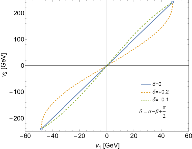
and apply the path deformation method [42, 35] to find the solution. However, in the alignment limit, the correct path is simply the straight line connecting the two minima in the field space (the blue path in Fig. 1a). Indeed, once we choose the path to be and , Eq. (9) is automatically satisfied regardless of the relation between and (see Appendix B for details). Then the problem is reduced to finding the domain wall solution for Eq. (8), which is simply
| (10) |
with GeV the mass of the SM-like Higgs and the SM Higgs quartic coupling. Here we have taken . Eq. (10) admits a well-known analytical solution [43]
| (11) |
where is the thickness of the wall. As usual, the surface energy density of the wall is
| (12) |
which is around given the SM Higgs VEV and self coupling.
2.2 Deviation from the alignment limit
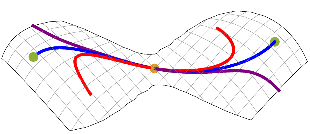
Although the experiments indicate the alignment limit is a good approximation, a deviation has not been ruled out yet. Allowing a deviation from the alignment limit, the domain wall solution would no longer follow the straight line between the two equivalent minima (see Appendix B for details). The domain wall solution can be found by the path deformation method (see for example [42, 35]), or alternatively, by the overshoot/undershoot method (see for example [44, 42]). As the scalar potential possesses a central symmetry, the domain wall path has to pass the center, which is the origin. The magnitude of the field profile derivative can be determined everywhere in the field space as in the spirit of the overshoot/undershoot method. Eventually the problem is reduced to finding the direction of the path at the origin. The path exactly connect the two minima for the correct direction, while the wrong direction never pass the minima without any ends, as shown in Fig. 2.
Using both methods, we solve the coupled system of field equations (8) and (9), and explore how much a deviation from the SM-like Higgs limit can change the domain wall energy density.
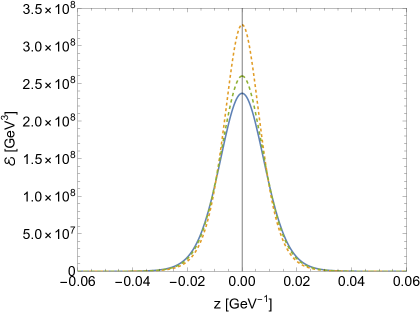
An illustrative example of this is shown in Fig. 1a. After the spontaneous symmetry breaking, there are five physical scalar fields, namely, two neutral scalars (one of which, , aligns with the SM Higgs in the alignment limit), a charged scalar, and a pseudoscalar. For the present example, we choose a benchmark point where the masses of the neutral scalar different from the SM-like Higgs, the charged scalar and the pseudoscalar are GeV, GeV and GeV, respectively, while . Details on the relations between the masses of physical scalar fields and model parameters are discussed in Appendix A. The path in the field space for the domain wall solution follows a straight line in the perfect alignment limit, as shown in Fig. 1a. On the other hand, allowing a deviation from the alignment limit, i.e., , the path changes. In particular, we consider two extremes of the deviation angle and which would reduce the coupling between and gauge bosons by around 2% and 0.5%, respectively.555A deviation from the alignment limit changes both the gauge interaction () and the Yukawa interaction () of by a factor . and correspond to and , respectively. Such deviations represent the limit allowed by the the experimental constraints [38, 37] while preserving the stability of the vacua.666A deviation leads to metastable vacua for the benchmark case. The energy density in the direction perpendicular to the wall is presented in Fig. 1b. In the presence of the deviation, the energy at the center of the domain wall becomes larger, leading to an increase in the total surface energy density. However, we find that the variation of the domain wall surface energy density is only about , leading to a negligible effect in the gravitational wave phenomenology.
3 Domain walls bounded by cosmic strings
In the type-I 2HDM extended by a gauged , the symmetry breaking pattern is as follows. The scalar gets a nonzero VEV at a high scale and gives large mass to the right-handed neutrino. This spontaneously breaks the symmetry and creates a cosmic string network [45]. We assume that this happens in a radiation dominated Universe after inflation has ended. This ensures that the string network is not diluted by inflation. 777Unlike other topological defects, string networks are not completely diluted away by inflation, and can even regrow to generate observable gravitational wave signatures. See [46, 47, 48] for details. In case that the string is completely diluted, hybrid topological defects can still appear through nucleation of holes bounded by strings on the domain wall [49, 50]. However, such topological defects can only lead to observable gravitational wave for quasi-degenerate string scale and wall scale, with inflation scale in the middle.
Because of the charge assignment of the fields, as given in Table 1, the model has a residual symmetry at the vacuum, under which both Higgs doublets and are odd. When either of them gets a nonzero VEV, the symmetry is spontaneously broken, leading to the creation of a domain wall network [45].
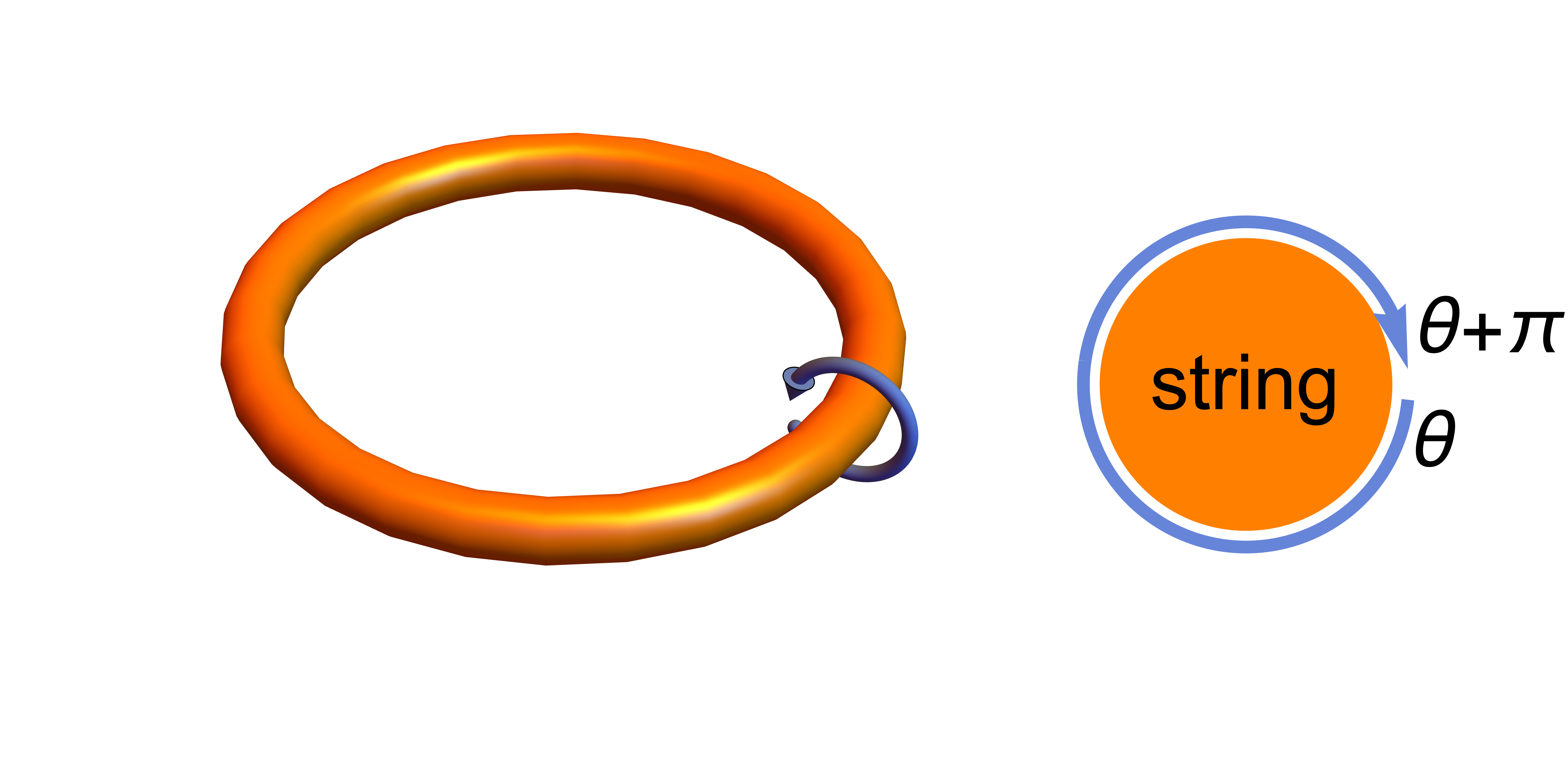
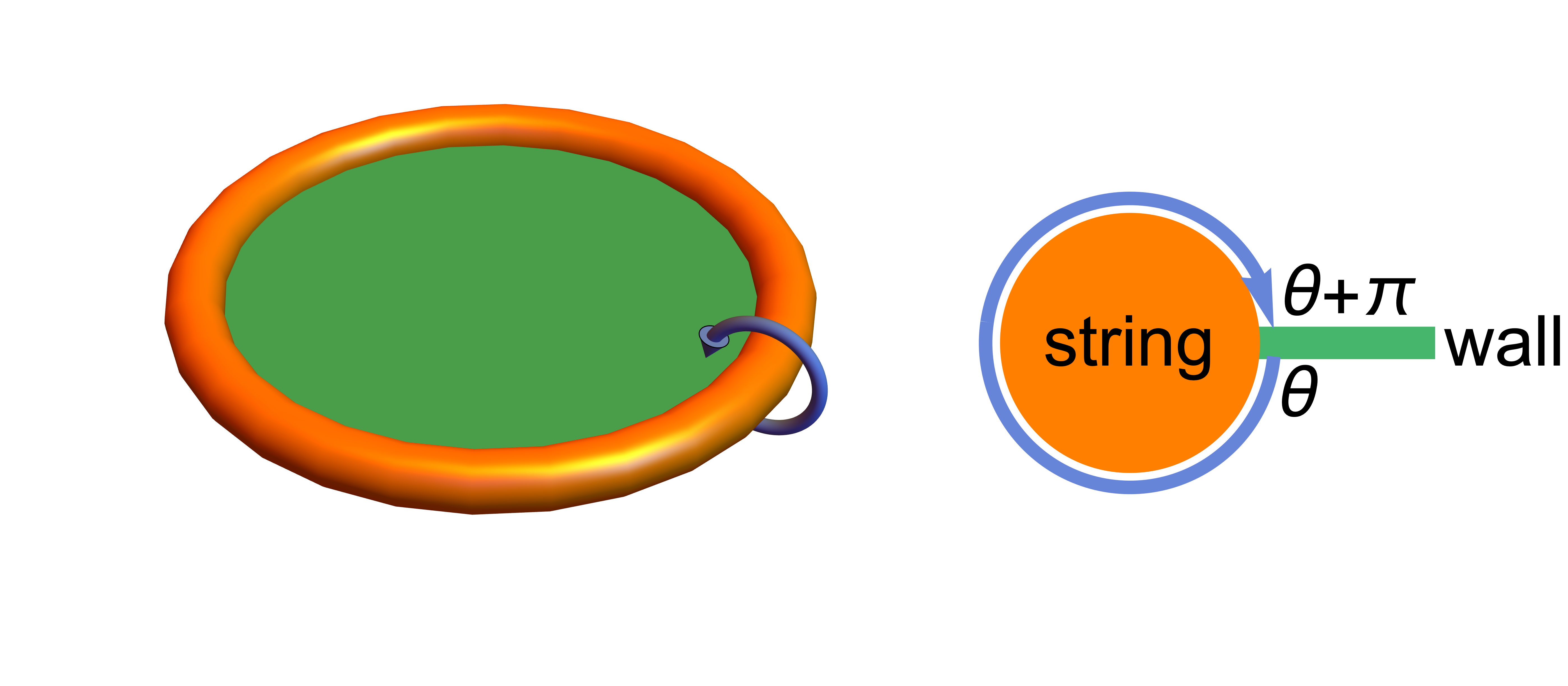
While the creation of cosmic strings and domain walls from their respective symmetry breakings have been widely studied in the context of various BSM models, the situation above is somewhat different. Here the is not a symmetry of the original Lagrangian, but is a residual symmetry that occurs at an intermediate stage in the symmetry breaking chain. When the symmetry is broken, the VEV of the scalar field with charge 2 can have a phase that can vary between and with the spacetime. The same applies to the other fields in the theory. After the symmetry breaking, the phase changes from to around a string, as shown in Fig. LABEL:fig2a. However, those fields with charge 1 are not invariant when changes to . Instead, there is a sign change in those fields, leading to a residual symmetry. As such, the created domain walls after breaking are not infinite planar walls, rather circular walls that fill in the space between string loops, as shown in Fig. LABEL:fig2b.888We focus on string loops. In case that the wall is formed between long strings, the wall would promote the loop formation [51]. This creates a hybrid topological defect dubbed as “walls bounded by strings” [52].
A detailed description of the evolution of this hybrid topological defect can be found in Ref. [53]. Here we will briefly discuss the relevant physics and the observational signatures of the defect.
A useful parameter that dictates the evolution of the defect is defined as , where is the string tension, being the breaking scale, and is the surface energy density of the domain wall, being the breaking scale, and assuming a coupling constant of the scalar field breaking . After the symmetry breaking, horizon size long strings are created that intersect and form string loops. These circular loops oscillate non-relativistically and lose their energy by emitting gravitational waves. When domain walls are formed at , where , and fill up the space between the string loops, they tend to make the string motion ultra-relativistic as long as the loop size is above . This makes the wall-string network collapse earlier than the case of pure string loops. If , walls do not dominate the string dynamics immediately after creation. As such, the hybrid network becomes ultra-relativistic and collapses after some time, . On the other hand, if , the hybrid network becomes ultra-relativistic as soon as the walls are created and the network collapses at . We can, therefore, define the time for the collapse of the hybrid network as [54].
For a loop of radius with circular length , the rate of energy loss is given by
| (13) |
where is the Newton’s constant. The function when in the pure string limit, and for in the pure wall limit. The behavior around can be approximated using a smooth interpolation function, as shown in Ref. [53].
Because of the energy loss, loops forming at time with an initial size slowly decrease in size with time. Here is the ratio between loop formation length and horizon size, and its value is determined from simulations [55, 56]. For the domain walls bounded by strings, the size of a string loop emitting gravitational waves at time is , and we have
| (14) |
Here the integration variable can be interpreted as the instantaneous length of the loop emitting gravitational wave at time , where . We further assume that at time , the newly created loops are larger than the pre-existing loops emitting gravitational wave at time
| (15) |
We can decompose the gravitational wave into Fourier modes , where the parameter varies between in the pure string limit () and in the pure wall limit [53]. This mode is redshifted to the frequency in today’s interferometers
| (16) |
where is the scale factor which is defined as where is the present time.
The gravitational wave spectrum observed today is given by summing over all Fourier modes
| (17) |
Here is the critical energy density today. s is the time when the network reaches a scaling regime where the energy density of the hybrid network becomes constant in the expanding Universe. is the fraction of energy that is transferred by the string network into loops [56]. is the loop formation efficiency which equals during the radiation-dominated era, and during the matter-dominated era. is the fractional power radiated by the th mode of an oscillating string loop with cusp, and is the Riemann zeta function. The power spectral index is found to be for string loops containing cusps [57, 58].
In Eq. (17), we are integrating over the gravitational wave modes emitted by the hybrid network from an early time when the network goes to a scaling regime, , to today . Here the integration variable represents the time when a loop is radiating gravitational wave, and is the time when this particular loop was created, which can be obtained by solving Eq. (14). The Heaviside function ensures that we only sum over the contribution from loops which were created before the network collapses at .
We have developed a public code package CosmicStringGW, available on GitHub at \faGithubSquare/moinulrahat/CosmicStringGW, for calculating the gravitational wave spectrum from pure and hybrid defect networks of cosmic strings.
4 Gravitational wave signature
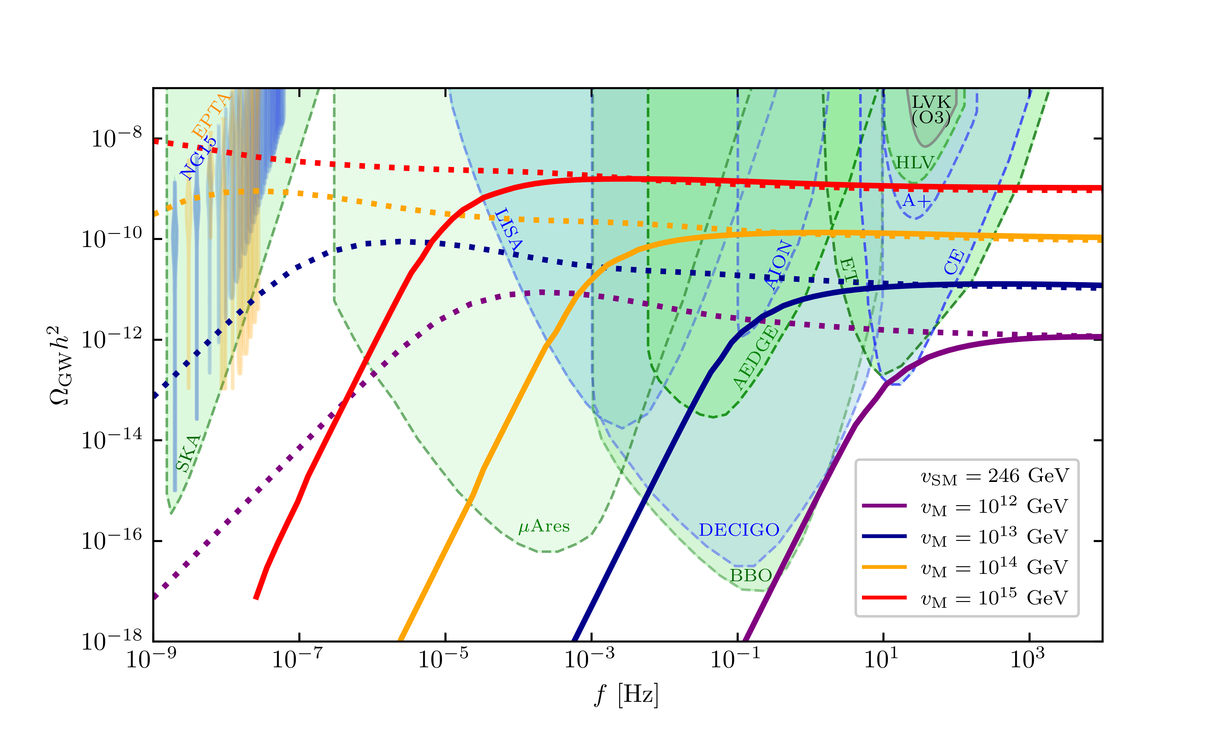
We expect the symmetry to be spontaneously broken at a high scale above GeV, inspired by a high scale of right-handed neutrino masses, and the symmetry to be broken at the electroweak scale. Hence we focus on keeping the breaking scale fixed at GeV, while varying the breaking scale.999We will adopt the perfect alignment limit when calculating the domain wall energy density, as we have verified that the allowed deviation has unnoticeable impact on the gravitational wave signals. The resulting gravitational waves from the string-wall network, calculated from evaluating Eq. (17) up to terms, is shown in Fig. 4 with solid lines. In the same plot we also show the spectrum corresponding to the pure string case, if the symmetry were completely broken at the high scale.101010This is achieved by taking the limit in Eq. (17). Projected sensitivity (SKA [59], -Ares [60], LISA [61], DECIGO [62, 63], BBO [64], AEDGE [65], AION [66], CE [67], ET [68] and future upgrades of LVK), upper bounds (LVK [69, 70, 71]) from various interferometers and recent results from pulsar timing arrays NANOGrav [72, 73] and EPTA [74, 75] are shown for comparison. Astrophysical foregrounds for the relevant frequency range are not shown, and can be found in Ref. [76]. Signal-to-noise ratio (SNR) at some of the detectors is tabulated in Appendix C.
We notice the following key characteristics of the gravitational wave spectrum generated from the hybrid network of domain walls bounded by cosmic strings.
-
•
Compared to the pure string case (dotted line), the signals from the hybrid network (solid line) have an infrared (IR) tail at larger frequencies. This is caused by the collapse of the network after creation of the domain walls that drive the boundary strings to ultra-relativistic dynamics. The frequency where the IR tail starts is determined by the collapse time , which in our model depends on (since for GeV). Higher implies that the collapse happens later, allowing the flat part of the signal to continue to lower frequencies (see Fig.4).
-
•
The spectral slope of the hybrid-defect signal is steeper compared to the pure string case. This has important implications for interferometers. The steep slope of the IR tail can be distinguished from the pure string case in planned interferometer sensitivities in the Hz to Hz frequencies.
-
•
The IR tail appearing at relatively higher frequencies compared to the pure string case implies that non-observation at pulsar timing arrays (PTA) does not rule out signals from the hybrid defect for GeV. The upper bound GeV from LVK applies to gravitational waves from both pure and hybrid cosmic string defects, as both signals are identical at LVK frequencies.
-
•
While the pure string signal probes a single symmetry breaking scale [77, 78, 79, 80, 81], signals from hybrid defects like domain walls bounded by cosmic strings can simultaneously probe two symmetry breaking scales ( and ). This offers a unique opportunity to test BSM scenarios where such scales are separated by orders of magnitude.
-
•
Given that the breaking scale in the current model is fixed at the electroweak scale, the model predicts a signal with spectral slope in the Hz to Hz range for breaking scale GeV. Together with a flat spectrum at frequencies higher than the IR tail, this is a unique signature of this model.
In summary, the hybrid network generated from the sequential breaking of the symmetry via the intermediate symmetry results in a unique GW signal distinguishable from other new physics signals in the observable frequency range, and can be probed in upcoming GW interferometers.
5 Conclusion
We have investigated the emergence of a hybrid topological defect, namely “domain walls bounded by cosmic strings”, and the unique gravitational wave signal that emerges from it in the context of the type-I two-Higgs-doublet model (2HDM) extended with a gauged symmetry. The phenomenological motivation for the extension stems from the necessity to incorporate neutrino masses and mixings via the seesaw mechanism. The model simultaneously cancels the chiral anomaly and eliminates the flavour-changing neutral currents. An interesting outcome of the charge assignment, motivated by spontaneous generation of the right-handed neutrino Majorana masses, is that is broken to an intermediate symmetry, which is further broken around the electroweak scale by the Higgs doublets. Such a chain of symmetry breaking triggers a hybrid topological defect of “domain walls bounded by cosmic strings”, created by the domain walls of breaking being encircled by pre-existing cosmic string loops originated from the earlier breaking.
We have studied the cosmological footprint of this model in terms of the decay of the hybrid network of walls bounded by strings into gravitational waves. The defect network evolves by losing energy via gravitation wave emission, where the observable frequency of the signal is inversely proportional to the time of evolution. The decay of the cosmic string loops created after breaking yields a flat spectrum of gravitational waves at high frequencies. The additional tension exerted by the bounded domain walls arising after breaking causes an accelerated decay of the loops, resulting in a characteristic slope of the signal in lower frequencies. The pivot frequency where this spectral change occurs is determined by the ratio of the two symmetry breaking scales, while the high frequency flat amplitude is representative of the higher scale. In the present model, the is broken around the electroweak scale. This leads to a prediction for the behaviour to be observed in the microHz to Hz band with a flat spectrum in the ultraviolet, when the breaking scale is in between GeV to GeV. In this sense, our study provides a way to test the model in upcoming gravitational wave interferometers such as LISA and ET, complementing the collider results.
Acknowledgement
We thank Yongcheng Wu for helpful discussions. MHR acknowledges financial support from the Spanish AEI-MICINN PID2020-113334GB-I00/AEI/10.13039/501100011033 and Generalitat Valenciana project CIPROM/2021/054. SFK thanks CERN for hospitality and acknowledges the STFC Consolidated Grant ST/L000296/1 and the European Union’s Horizon 2020 Research and Innovation programme under Marie Skłodowska-Curie grant agreement HIDDeN European ITN project (H2020-MSCA-ITN-2019//860881-HIDDeN).
Appendix A The scalar sector of 2HDM
The minimisation conditions for the Higgs potential are given by
| (18a) | ||||
| (18b) | ||||
where . After the spontaneous symmetry breaking, there are five physical scalar fields: two neutral scalars ( and ), a charged scalar (), and one pseudoscalar (). The mass spectrum of the scalar particles are
| (19) | ||||
| (20) | ||||
| (21) |
where and .
In total, there are 7 model parameters and 7 physical parameters in the Higgs sector, as listed in Table 2.
| Model parameters | Physical parameters |
|---|---|
The physical parameters and the model parameters are related by
| (22) | ||||
| (23) | ||||
| (24) | ||||
| (25) | ||||
| (26) | ||||
| (27) | ||||
| (28) |
In the alignment limit, these relations between model and physical parameters are reduced to
| (29) |
The stability of the vacuum can be ensured by , and .
Appendix B Equations of motion for domain wall in the Higgs basis
In the 2HDM, there is a basis of the Higgs doublets under which only one of the Higgs doublets obtains a VEV, which is known as the Higgs basis. The Higgs basis can be obtained by the following rotation of the fields:
| (30) |
In the Higgs basis, the scalar potential Eq. (5) would be minimised at , where .
Under the alignment limit, the path of the field value for the domain wall solution happens to be a straight line connecting the two symmetric vacua. Along the direction (), the gradient of the potential reads
| (31) |
where is the mass of . Therefore the equation of motion for , which is , is automatically satisfied when . In this case, the domain wall solution can be obtained by solving the equation of motion for .
However, in the more general case without the alignment limit, it is not necessary that only one Higgs boson gets VEV everywhere in the domain wall solution for 2HDM. In that case, the gradient of the potential along the direction () is
| (32) | |||||
| (33) |
The equation of motion for is no longer trivial when . In order to get the correct domain wall solution, the path has to depart from the direction. Although only gets a VEV at the minima, the value of is non-zero inside the domain wall.
Appendix C Signal-to-noise ratio
We calculate the signal-to-noise ratio (SNR) of the gravitational wave signal from the hybrid topological defect at various interferometers as follows [82].
| SNR | (34) |
where denotes the sensitivity of the interferometers, is the GW signal, and is the duration of running in years. We take for all interferometers. In this definition, is taken to be the threshold for detection in a given interferometer [82]. The resulting SNR is shown in Table 3.
| Interferometer | GeV | GeV | GeV | GeV |
| ARES | 0.0 | 0.0 | ||
| LISA | 0.0 | 0.01 | 343.51 | |
| BBO | 3.46 | |||
| DECIGO | 2.43 | |||
| AION | 0.0 | 0.97 | 57.51 | 630.99 |
| AEDGE | 0.0 | 15.19 | ||
| ET | 7.21 | 379.58 | ||
| CE | 12.79 | 654.21 | ||
| A+ | 0.01 | 0.24 | 2.58 | 22.55 |
| HLV | 0.0 | 0.07 | 0.71 | 6.25 |
References
- [1] ATLAS collaboration, Observation of a new particle in the search for the Standard Model Higgs boson with the ATLAS detector at the LHC, Phys. Lett. B 716 (2012) 1 [1207.7214].
- [2] CMS collaboration, Observation of a New Boson at a Mass of 125 GeV with the CMS Experiment at the LHC, Phys. Lett. B 716 (2012) 30 [1207.7235].
- [3] CMS collaboration, Search for a standard model-like Higgs boson in the mass range between 70 and 110 GeV in the diphoton final state in proton-proton collisions at 8 and 13 TeV, Phys. Lett. B 793 (2019) 320 [1811.08459].
- [4] ILC collaboration, H. Baer et al., eds., The International Linear Collider Technical Design Report - Volume 2: Physics, 1306.6352.
- [5] F. An et al., Precision Higgs physics at the CEPC, Chin. Phys. C 43 (2019) 043002 [1810.09037].
- [6] M. Cepeda et al., Report from Working Group 2: Higgs Physics at the HL-LHC and HE-LHC, CERN Yellow Rep. Monogr. 7 (2019) 221 [1902.00134].
- [7] T.D. Lee, A Theory of Spontaneous T Violation, Phys. Rev. D 8 (1973) 1226.
- [8] S.L. Glashow and S. Weinberg, Natural Conservation Laws for Neutral Currents, Phys. Rev. D 15 (1977) 1958.
- [9] E.A. Paschos, Diagonal Neutral Currents, Phys. Rev. D 15 (1977) 1966.
- [10] G.C. Branco, P.M. Ferreira, L. Lavoura, M.N. Rebelo, M. Sher and J.P. Silva, Theory and phenomenology of two-Higgs-doublet models, Phys. Rept. 516 (2012) 1 [1106.0034].
- [11] I.P. Ivanov, Building and testing models with extended Higgs sectors, Prog. Part. Nucl. Phys. 95 (2017) 160 [1702.03776].
- [12] P. Ko, Y. Omura and C. Yu, A Resolution of the Flavor Problem of Two Higgs Doublet Models with an Extra Symmetry for Higgs Flavor, Phys. Lett. B 717 (2012) 202 [1204.4588].
- [13] P. Ko, Y. Omura and C. Yu, Higgs phenomenology in Type-I 2HDM with Higgs gauge symmetry, JHEP 01 (2014) 016 [1309.7156].
- [14] P. Ko, Y. Omura and C. Yu, Dark matter and dark force in the type-I inert 2HDM with local U(1)H gauge symmetry, JHEP 11 (2014) 054 [1405.2138].
- [15] M.D. Campos, D. Cogollo, M. Lindner, T. Melo, F.S. Queiroz and W. Rodejohann, Neutrino Masses and Absence of Flavor Changing Interactions in the 2HDM from Gauge Principles, JHEP 08 (2017) 092 [1705.05388].
- [16] P. Minkowski, at a Rate of One Out of Muon Decays?, Phys. Lett. B 67 (1977) 421.
- [17] T. Yanagida, Horizontal gauge symmetry and masses of neutrinos, Proceedings of the Workshop on Unified Theory and Baryon Number of the Universe, (1979) .
- [18] M. Gell-Mann, P. Ramond and R. Slansky, in Sanibel talk, retroprinted as [9809459], and in Supergravity, North-Holland, Amsterdam (1979), PRINT-80-0576, retroprinted as [1306.4669], .
- [19] S. Glashow, The Future of Elementary Particle Physics, NATO Sci. Ser. B 61 (1980) 687.
- [20] R.N. Mohapatra and G. Senjanovic, Neutrino Mass and Spontaneous Parity Nonconservation, Phys. Rev. Lett. 44 (1980) 912.
- [21] A. Arhrib, R. Benbrik and S. Moretti, Bosonic Decays of Charged Higgs Bosons in a 2HDM Type-I, Eur. Phys. J. C 77 (2017) 621 [1607.02402].
- [22] A. Arhrib, R. Benbrik, S. Moretti, A. Rouchad, Q.-S. Yan and X. Zhang, Multi-photon production in the Type-I 2HDM, JHEP 07 (2018) 007 [1712.05332].
- [23] R. Enberg, W. Klemm, S. Moretti and S. Munir, Signatures of the Type-I 2HDM at the LHC, PoS CORFU2018 (2018) 013 [1812.08623].
- [24] Y. Wang, A. Arhrib, R. Benbrik, M. Krab, B. Manaut, S. Moretti et al., Analysis of W± + 4 in the 2HDM Type-I at the LHC, JHEP 12 (2021) 021 [2107.01451].
- [25] Y. Wang, A. Arhrib, R. Benbrik, M. Krab, B. Manaut, S. Moretti et al., Searching for signals in the 2HDM Type-I at the LHC, 11, 2021 [2111.12286].
- [26] S. Moretti, S. Semlali and C.H. Shepherd-Themistocleous, A novel experimental search channel for very light higgs bosons in the 2HDM type I, Eur. Phys. J. C 84 (2024) 245 [2207.03007].
- [27] S. Moretti, S. Semlali and C.H. Shepherd-Themistocleous, Hunting light Higgses at the LHC in the context of the 2HDM Type-I, PoS ICHEP2022 (2022) 529 [2211.11388].
- [28] T. Mondal, S. Moretti, S. Munir and P. Sanyal, Electroweak Multi-Higgs Production: A Smoking Gun for the Type-I Two-Higgs-Doublet Model, Phys. Rev. Lett. 131 (2023) 231801 [2304.07719].
- [29] A. Arhrib, S. Moretti, S. Semlali, C.H. Shepherd-Themistocleous, Y. Wang and Q.S. Yan, Searching for H→hh→bb¯ in the 2HDM type-I at the LHC, Phys. Rev. D 109 (2024) 055020 [2310.02736].
- [30] W. Liu, L. Wang and Y. Zhang, Direct Production of Light Scalar in the Type-I Two-Higgs-Doublet Model at the Lifetime Frontier of LHC, 2403.16623.
- [31] N. Chen, T. Han, S. Li, S. Su, W. Su and Y. Wu, Type-I 2HDM under the Higgs and Electroweak Precision Measurements, JHEP 08 (2020) 131 [1912.01431].
- [32] T. Han, S. Li, S. Su, W. Su and Y. Wu, Heavy Higgs bosons in 2HDM at a muon collider, Phys. Rev. D 104 (2021) 055029 [2102.08386].
- [33] T. Han, S. Li, S. Su, W. Su and Y. Wu, Comparative Studies of 2HDMs under the Higgs Boson Precision Measurements, JHEP 01 (2021) 045 [2008.05492].
- [34] L. Bian, N. Chen, W. Su, Y. Wu and Y. Zhang, Future prospects of mass-degenerate Higgs bosons in the CP -conserving two-Higgs-doublet model, Phys. Rev. D 97 (2018) 115007 [1712.01299].
- [35] N. Chen, T. Li, Z. Teng and Y. Wu, Collapsing domain walls in the two-Higgs-doublet model and deep insights from the EDM, JHEP 10 (2020) 081 [2006.06913].
- [36] L. Delle Rose, S. Khalil and S. Moretti, Explanation of the 17 MeV Atomki anomaly in a U(1)’ -extended two Higgs doublet model, Phys. Rev. D 96 (2017) 115024 [1704.03436].
- [37] ATLAS collaboration, A detailed map of Higgs boson interactions by the ATLAS experiment ten years after the discovery, Nature 607 (2022) 52 [2207.00092].
- [38] CMS collaboration, A portrait of the Higgs boson by the CMS experiment ten years after the discovery., Nature 607 (2022) 60 [2207.00043].
- [39] J.F. Gunion and H.E. Haber, The CP conserving two Higgs doublet model: The Approach to the decoupling limit, Phys. Rev. D 67 (2003) 075019 [hep-ph/0207010].
- [40] H.E. Haber, A natural mechanism for a SM-like Higgs boson in the 2HDM without decoupling, PoS DISCRETE2020-2021 (2022) 010 [2205.07578].
- [41] K. Saikawa, A review of gravitational waves from cosmic domain walls, Universe 3 (2017) 40 [1703.02576].
- [42] C.L. Wainwright, CosmoTransitions: Computing Cosmological Phase Transition Temperatures and Bubble Profiles with Multiple Fields, Comput. Phys. Commun. 183 (2012) 2006 [1109.4189].
- [43] E.W. Kolb and M.S. Turner, eds., THE EARLY UNIVERSE. REPRINTS (1988).
- [44] R. Apreda, M. Maggiore, A. Nicolis and A. Riotto, Gravitational waves from electroweak phase transitions, Nucl. Phys. B 631 (2002) 342 [gr-qc/0107033].
- [45] T.W.B. Kibble, Topology of Cosmic Domains and Strings, J. Phys. A 9 (1976) 1387.
- [46] G.S.F. Guedes, P.P. Avelino and L. Sousa, Signature of inflation in the stochastic gravitational wave background generated by cosmic string networks, Phys. Rev. D 98 (2018) 123505 [1809.10802].
- [47] Y. Cui, M. Lewicki and D.E. Morrissey, Gravitational Wave Bursts as Harbingers of Cosmic Strings Diluted by Inflation, Phys. Rev. Lett. 125 (2020) 211302 [1912.08832].
- [48] F. Ferrer, A. Ghoshal and M. Lewicki, Imprints of a supercooled phase transition in the gravitational wave spectrum from a cosmic string network, JHEP 09 (2023) 036 [2304.02636].
- [49] T.W.B. Kibble, G. Lazarides and Q. Shafi, Strings in SO(10), Phys. Lett. B 113 (1982) 237.
- [50] T.W.B. Kibble, G. Lazarides and Q. Shafi, Walls Bounded by Strings, Phys. Rev. D 26 (1982) 435.
- [51] L. Leblond, B. Shlaer and X. Siemens, Gravitational Waves from Broken Cosmic Strings: The Bursts and the Beads, Phys. Rev. D 79 (2009) 123519 [0903.4686].
- [52] A.E. Everett and A. Vilenkin, Left-right Symmetric Theories and Vacuum Domain Walls and Strings, Nucl. Phys. B 207 (1982) 43.
- [53] D.I. Dunsky, A. Ghoshal, H. Murayama, Y. Sakakihara and G. White, GUTs, hybrid topological defects, and gravitational waves, Phys. Rev. D 106 (2022) 075030 [2111.08750].
- [54] X. Martin and A. Vilenkin, Gravitational wave background from hybrid topological defects, Phys. Rev. Lett. 77 (1996) 2879 [astro-ph/9606022].
- [55] J.J. Blanco-Pillado and K.D. Olum, Stochastic gravitational wave background from smoothed cosmic string loops, Phys. Rev. D 96 (2017) 104046 [1709.02693].
- [56] J.J. Blanco-Pillado, K.D. Olum and B. Shlaer, The number of cosmic string loops, Phys. Rev. D 89 (2014) 023512 [1309.6637].
- [57] P. Auclair et al., Probing the gravitational wave background from cosmic strings with LISA, JCAP 04 (2020) 034 [1909.00819].
- [58] T. Vachaspati and A. Vilenkin, Gravitational Radiation from Cosmic Strings, Phys. Rev. D 31 (1985) 3052.
- [59] G. Janssen et al., Gravitational wave astronomy with the SKA, PoS AASKA14 (2015) 037 [1501.00127].
- [60] A. Sesana et al., Unveiling the gravitational universe at -Hz frequencies, Exper. Astron. 51 (2021) 1333 [1908.11391].
- [61] LISA collaboration, Laser Interferometer Space Antenna, 1702.00786.
- [62] H. Kudoh, A. Taruya, T. Hiramatsu and Y. Himemoto, Detecting a gravitational-wave background with next-generation space interferometers, Phys. Rev. D 73 (2006) 064006 [gr-qc/0511145].
- [63] S. Kawamura et al., Current status of space gravitational wave antenna DECIGO and B-DECIGO, PTEP 2021 (2021) 05A105 [2006.13545].
- [64] G.M. Harry, P. Fritschel, D.A. Shaddock, W. Folkner and E.S. Phinney, Laser interferometry for the big bang observer, Class. Quant. Grav. 23 (2006) 4887.
- [65] AEDGE collaboration, AEDGE: Atomic Experiment for Dark Matter and Gravity Exploration in Space, EPJ Quant. Technol. 7 (2020) 6 [1908.00802].
- [66] L. Badurina et al., AION: An Atom Interferometer Observatory and Network, JCAP 05 (2020) 011 [1911.11755].
- [67] LIGO Scientific collaboration, Exploring the Sensitivity of Next Generation Gravitational Wave Detectors, Class. Quant. Grav. 34 (2017) 044001 [1607.08697].
- [68] S. Hild, S. Chelkowski and A. Freise, Pushing towards the ET sensitivity using ’conventional’ technology, 0810.0604.
- [69] LIGO Scientific, VIRGO, KAGRA collaboration, Search for gravitational-wave transients associated with magnetar bursts in Advanced LIGO and Advanced Virgo data from the third observing run, 2210.10931.
- [70] KAGRA, Virgo, LIGO Scientific collaboration, Upper limits on the isotropic gravitational-wave background from Advanced LIGO and Advanced Virgo’s third observing run, Phys. Rev. D 104 (2021) 022004 [2101.12130].
- [71] Y. Jiang and Q.-G. Huang, Upper limits on the polarized isotropic stochastic gravitational-wave background from advanced LIGO-Virgo’s first three observing runs, JCAP 02 (2023) 026 [2210.09952].
- [72] NANOGrav collaboration, The NANOGrav 15 yr Data Set: Evidence for a Gravitational-wave Background, Astrophys. J. Lett. 951 (2023) L8 [2306.16213].
- [73] NANOGrav collaboration, The NANOGrav 15 yr Data Set: Search for Signals from New Physics, Astrophys. J. Lett. 951 (2023) L11 [2306.16219].
- [74] EPTA collaboration, The second data release from the European Pulsar Timing Array - I. The dataset and timing analysis, Astron. Astrophys. 678 (2023) A48 [2306.16224].
- [75] EPTA, InPTA: collaboration, The second data release from the European Pulsar Timing Array - III. Search for gravitational wave signals, Astron. Astrophys. 678 (2023) A50 [2306.16214].
- [76] I. Baldes and M.O. Olea-Romacho, Primordial black holes as dark matter: interferometric tests of phase transition origin, JHEP 01 (2024) 133 [2307.11639].
- [77] J.A. Dror, T. Hiramatsu, K. Kohri, H. Murayama and G. White, Testing the Seesaw Mechanism and Leptogenesis with Gravitational Waves, Phys. Rev. Lett. 124 (2020) 041804 [1908.03227].
- [78] A. Dasgupta, P.S.B. Dev, A. Ghoshal and A. Mazumdar, Gravitational wave pathway to testable leptogenesis, Phys. Rev. D 106 (2022) 075027 [2206.07032].
- [79] B. Fu, A. Ghoshal and S.F. King, Cosmic string gravitational waves from global symmetry breaking as a probe of the type I seesaw scale, JHEP 11 (2023) 071 [2306.07334].
- [80] P. Di Bari, S.F. King and M.H. Rahat, Gravitational waves from phase transitions and cosmic strings in neutrino mass models with multiple Majorons, 2306.04680.
- [81] S.F. King, D. Marfatia and M.H. Rahat, Toward distinguishing Dirac from Majorana neutrino mass with gravitational waves, Phys. Rev. D 109 (2024) 035014 [2306.05389].
- [82] C. Caprini et al., Science with the space-based interferometer eLISA. II: Gravitational waves from cosmological phase transitions, JCAP 04 (2016) 001 [1512.06239].